Design of near-infrared imaging probe with the assistance of ultrasound localization

Abstract

A total of 364 optical source–detector pairs were deployed uniformly over a 9 cm × 9 cm probe area initially, and then the total pairs were reduced gradually to 60 in experimental and simulation studies. For each source–detector configuration, three-dimensional (3-D) images of a 1-cm-diameter absorber of different contrasts were reconstructed from the measurements made with a frequency-domain system. The results have shown that more than 160 source–detector pairs are needed to reconstruct the absorption coefficient to within 60% of the true value and appropriate spatial and contrast resolution. However, the error in target depth estimated from 3-D images was more than 1 cm in all source–detector configurations. With the a priori target depth information provided by ultrasound, the accuracy of the reconstructed absorption coefficient was improved by 15% and 30% on average, and the beam width was improved by 24% and 41% on average for high- and low-contrast cases, respectively. The speed of reconstruction was improved by ten times on average.

1. Introduction

Recently, optical imaging techniques based on diffusive near-infrared (NIR) light have been employed to obtain interior optical properties of human tissues.^1–8 Functional imaging with NIR light has the potential to detect and diagnose diseases or cancers through the determination of hemoglobin concentration, blood O₂ saturation, tissue light scattering, water concentration, and the concentration and lifetime of exogenous contrast agents. Optical imaging requires that an array of sources and detectors be distributed directly or coupled through optical fibers on a boundary surface. Measurements made at all source–detector positions can be used in tomographic image reconstruction schemes to determine optical properties of the medium. The frequently used geometric configurations of sources and detectors are ring arrays^4,9–11 and planar arrays.^3,12–15 A ring array consists of multiple sources and detectors that can be distributed uniformly on a ring. Optical properties of the thin tissue slice (two-dimensional slice) enclosed by the ring can be determined from all measurements. A planar array can be configured with either transmission or reflection geometries. In transmission geometry, multiple detectors can be deployed on a planar array, and multiple sources or a single source can be deployed on an opposite plane parallel to the detector plane. Optical properties of the three-dimensional (3-D) tissue volume between the source and the detector planes can be determined from all measurements. In reflection geometry, multiple sources and detectors can be distributed on a planar probe that can be hand-held.^3,15 Optical properties of the 3-D tissue volume at slice depths below the probe can be determined from all measurements. The reflection probe configuration is desirable for the imaging of brain and breast tissues.

Although many researchers in the field have constructed imaging probes using reflection geometry,^2,3,15 to our knowledge the required total number of source–detector pairs over a given probe area needed to accurately reconstruct optical properties and localized spatial and depth distributions has not been addressed before. In this paper we study the relationship between the total number of source-detector pairs and the reconstructed imaging quality through experimental measurements. Computer simulations are performed to assist in understanding the experimental results.

Because the target localization from diffusive waves is difficult, our group and others have introduced use of a priori target location information provided by ultrasound to improve optical imaging.^15–18 In this paper we demonstrate experimentally that the accurate target depth information can significantly improve the accuracy of the reconstructed absorption coefficient and the reconstruction speed for any optical array configuration.

The required total number of source–detector pairs is also related to the image reconstruction algorithms used. In this paper we obtained experimental measurements using a frequency-domain system with the source amplitude modulated at 140 MHz. In simulations, forward measurements were generated by use of the analytic solution of a photon density wave scattered by a spherical inhomogeneity embedded in a semi-infinite scattering medium.¹⁹ In both experiments and simulations, linear perturbation theory within the Born approximation was used to relate optical signals at the probe surface to absorption variations in each volume element within the sample. The total least-squares (TLS) method^20–22 was used to formulate the inverse problem. The conjugate gradient technique was employed to iteratively solve the inverse problem. Therefore the results we obtained are directly relevant to the probe design with reconstruction algorithms based on the linear perturbation theory and can be used as a first-order approximation if high-order perturbations are employed in image reconstructions.

This paper is organized as follows. In Section 2 we describe an analytic solution used to generate simulated forward data, the Born approximation, and the TLS method for image reconstruction. In Section 3 we discuss the probe geometry, a frequency-domain NIR system used to acquire the experimental measurements, and an ultrasound subsystem used to acquire the target depth information, computation procedures used to obtain both simulated and experimental absorption images. In Sections 4 and 5 we report experimental results obtained from the dense and sparse arrays with and without a priori target depth information. A high-contrast example is given in Section 4, and a low-contrast case is given in Section 5. Simulations are performed to assist in understanding the noise on the image reconstruction. Imaging parameters evaluated are a −6-dB width of the image lobe, the reconstructed maximum value of the absorption coefficient and its spatial location, and the image artifact level. In Sections 6 and 7 we provide a discussion and summary, respectively.

2. Basic Principles

A. Forward Model

In our experiments, forward measurements were made with a frequency-domain system operating at a 140-MHz modulation frequency. In computer simulations, forward measurements were generated from an analytic solution of a photon density wave scattered by a spherical inhomogeneity.¹⁹ When the center of the sphere coincides with the origin of spherical coordinates, the solution for the scattered photon density wave U_sc outside the sphere at a detector position r = (r,θ,φ) is of the form

$$U_{\text{sc}}(\mathbf{r},\omega )=\sum _{l,m}\{A_{l,m}[j_l(k^{\text{out}}r)+{jn}_l(k^{\text{out}}r)]Y_{l,m}(\theta ,\phi )\},$$ (1)

where j_l and n_l are spherical Bessel and Neuman functions, respectively; Y_l,m(θ, φ) are the spherical harmonics, and k^out = [(−νμ_a^out + jω)/D^out]^1/2 is the complex wave number outside the sphere. ω is the angular modulation frequency of the light source, μ_a^out is the absorption coefficient outside the sphere, and D^out is the photon diffusion coefficient outside the sphere given by D^out = 1/(3μ_s′), where μ_s′ is the reduced scattering coefficient outside the sphere. The coefficients A_l,m, determined by the boundary conditions, are

$$A_{l,m}=-({\mathit{jvSk}}^{\text{out}}/D^{\text{out}})h_l^{(1)}(k^{\text{out}}{r}_s)Y_{l,m}\ast ({\theta }_s,{\phi }_s)\times \frac{D^{\text{out}}{xj}_l(y){j_l}^{\prime }(x)-D^{\text{in}}{{yj}_l}^{\prime }(y)j_l(x)}{D^{\text{out}}{{xh}_l^{(1)}}^{\prime }(x)j_l(y)-D^{\text{in}}{yh}_l^{(1)}(x){j_l}^{\prime }(y)},$$ (2)

where x = k^outa, y = kⁱⁿa, r_s = (r_s,θ_s,φ_s) is the source position, $h_l^{(1)}$ are the Hankel functions of the first kind, and ${j_l}^{\prime }$ and ${h_l^{(1)}}^{\prime }$ are the first derivatives of j_l and $h_l^{(1)}$. The analytic solution has the important advantage in that it is exact to all orders of perturbation theory and thus can represent accurate measurements.

We generalized the above analytic solution to a semi-infinite geometry by using a method of images with extrapolated boundary conditions (see Fig. 1). A type I boundary condition (zero light energy density at the extrapolated boundary) is used to derive the scattered wave U_sc′. To calculate the U_sc′ in semi-infinite geometry, we use r_sph+ = (r₀₊,θ₀₊, φ₀₊) and r_sph− = (r₀₋,θ₀₋,φ₀₋) to represent the centers of the sphere and the image sphere, respectively. The vectors r₊′ = r − r_sph+ = (r₊′, θ₊′, φ₊′) and r₋′ = r − r_sph− = (r₋′, θ₋′, φ₊′) are therefore pointing to the detector position r = (r, θ, φ) from the sphere and the image sphere, respectively. The semi-infinite solution of U_sc′ can be approximated as

Fig. 1.

Target, source, and detector configurations for a semi-infinite medium.

$$\begin{array}{l}{U_{\text{sc}}}^{\prime }(\mathbf{r},\omega )=\sum _{l,m}\{{A_{l,m}}^{+}[j_l(k^{\text{out}}{r_{+}}^{\prime })+{jn}_l(k^{\text{out}}{r_{+}}^{\prime })]Y_{l,m}({{\theta }_{+}}^{\prime },{{\phi }_{+}}^{\prime })\}\\ -\sum _{l,m}\{{A_{l,m}}^{-}[j_l(k^{\text{out}}{r_{+}}^{\prime })+{jn}_l(k^{\text{out}}{r_{+}}^{\prime })]Y_{l,m}({{\theta }_{+}}^{\prime },{{\phi }_{+}}^{\prime })\}\\ +\sum _{l,m}\{{A_{l,m}}^{+}[j_l(k^{\text{out}}{r_{-}}^{\prime })+{jn}_l(k^{\text{out}}{r_{-}}^{\prime })]Y_{l,m}({{\theta }_{-}}^{\prime },{{\phi }_{-}}^{\prime })\}\\ -\sum _{l,m}\{{A_{l,m}}^{-}[j_l(k^{\text{out}}{r_{-}}^{\prime })+{jn}_l(k^{\text{out}}{r_{-}}^{\prime })]Y_{l,m}({{\theta }_{-}}^{\prime },{{\phi }_{-}}^{\prime })\},\end{array}$$ (3)

where

$${A_{l,m}}^{+}=-({\mathit{jvSK}}^{\text{out}}/D^{\text{out}})h_l^{(1)}(k^{\text{out}}{r_s}^{+})Y_{l,m}\ast ({{\theta }_s}^{+},{{\phi }_s}^{+})\times \left[\frac{D^{\text{out}}{xj}_l(y){j_l}^{\prime }(x)-D^{\text{in}}{{yj}_l}^{\prime }(y)j_l(x)}{D^{\text{out}}{{xh}_l^{(1)}}^{\prime }(x)j_l(y)-D^{\text{in}}{yh}_l^{(1)}(x){j_l}^{\prime }(y)}\right],$$ (4)

$${A_{l,m}}^{-}=-({\mathit{jvSk}}^{\text{out}}/D^{\text{out}})h_l^{(1)}(k^{\text{out}}{r_s}^{+})Y_{l,m}\ast ({{\theta }_s}^{+},{{\phi }_s}^{+})\times \left[\frac{D^{\text{out}}{xj}_l(y){j_l}^{\prime }(x)-D^{\text{in}}{{yj}_l}^{\prime }(y)j_l(x)}{D^{\text{out}}{{xh}_l^{(1)}}^{\prime }(x)j_l(y)-D^{\text{in}}{yh}_l^{(1)}(x){j_l}^{\prime }(y)}\right].$$ (5)

r_s⁺ = (r_s⁺, θ_s⁺, φ_s⁺) and r_s⁻ = (r_s⁻, θ_s⁻, φ_s⁻) are the positions of the source and the image source, respectively.

The incident photon density wave at the detector position r has the following form³:

$$U_{\text{inc}}(\mathbf{r},\omega )=\frac{S}{4\pi D^{\text{out}}}\left[\frac{exp(j{k}^{\text{out}}\mid \mathbf{r}-{{\mathbf{r}}_s}^{+}\mid )}{\mid \mathbf{r}-{{\mathbf{r}}_s}^{+}\mid }-\frac{exp(j{k}^{\text{out}}\mid \mathbf{r}-{{\mathbf{r}}_s}^{-}\mid )}{\mid \mathbf{r}-{{\mathbf{r}}_s}^{-}\mid }\right].$$ (6)

The total photon density at detector r is a superposition of its incident (homogeneous) and scattered (heterogeneous) waves:

$$U(\mathbf{r},\omega )=U_{\text{inc}}(\mathbf{r},\omega )+{U_{\text{sc}}}^{\prime }(\mathbf{r},\omega ).$$ (7)

B. Born Approximation for Reconstruction

The Born approximation was used to relate U_sc′ (r,ω) measured at the probe surface to absorption variations in each volume element within the sample. In the Born approximation, the scattered wave that originated from a source at r_s and measured at detector r_d can be related to the medium heterogeneity Δμ_a (r_ν) by

$${U_{\text{sc}}}^{\prime }({\mathbf{r}}_{\text{d}},{\mathbf{r}}_s,\omega )=\int G({\mathbf{r}}_{\nu },{\mathbf{r}}_d,\omega )U_{\text{inc}}({\mathbf{r}}_{\nu },{\mathbf{r}}_s,\omega )\times [\nu \mathrm{\Delta }{\mu }_a({\mathbf{r}}_{\nu })/\overline{D}]\text{d}{r_{\nu }}^3,$$ (8)

where G(r_ν,r_d,ω) is the Green function and Δμ_a(r_ν) = μ_a(r_ν) − μ̄_a is the medium absorption variation.¹¹ μ̄_a is the average value of the medium absorption coefficient. By breaking the medium into discrete voxels, we obtain the following linear equations:

$${U_{\text{sc}}}^{\prime }({\mathbf{r}}_{\text{di}},{\mathbf{r}}_{\text{si}},\omega )=\sum _j^{N}G({\mathbf{r}}_{\text{vj}},{\mathbf{r}}_{\text{di}},\omega )U_{\text{inc}}({\mathbf{r}}_{\text{vj}},{\mathbf{r}}_{\text{si}},\omega )\times [\nu \mathrm{\Delta }{\mu }_a({\mathbf{r}}_{vj})/\overline{D}]\mathrm{\Delta }{r_{\nu }}^3.$$ (9)

When W_ij = G(r_νj,r_di,ω)U_inc (r_vj,r_si,ω)νΔr_ν³/D̄, we obtain the matrix equation of Eq. (9):

$${[W]}_{\mathit{MXN}}{\{\mathrm{\Delta }{\mu }_a\}}_{NX1}={[U_{\text{sd}}]}_{MX1}.$$ (10)

The realistic constrains on Δμ_a are (−α × background μ_a) = < Δμ_a < 1, where 0 < α <1.

The above constrains ensure that the reconstructed absorption coefficient μ̂_a = background μ_a + Δμ_a is positive and not unrealistically higher than unity. With M measurements obtained from all possible source–detector pairs in the planar array, we can solve N unknowns of Δμ_a by inverting the matrix Eq. (10). In general, the perturbation in Eq. (10) is underdetermined (M < N) and ill-posed.

When the target depth is available from ultrasound, we can set Δμ_a of a nontarget depth equal to zero. This implies that all the measured perturbations were originated from the particular depth that contained the target. Because the number of unknowns was reduced significantly, the reconstruction converged fast.

C. Total Least-Squares Solution

To solve the unknown optical properties of Eq. (10), several iterative algorithms have been used in the literature including the regularized least-squares method¹⁰ and the TLS method.^20,21 The TLS performs better than the regularized least-squares method when the measurement data are subject to noise and the linear operator W contains errors. The operator errors can result from both the approximations used to derive the linear model and the numerical errors in the computation of the operator. We found that the TLS method provides more accurate reconstructed optical properties than the regularized least-squares method, so we adapted the TLS method to solve the inverse problems. It has been shown by Golub²² that the TLS minimization is equivalent to the following minimization problem:

$$min\frac{{\left|\right|U_{\text{sd}}-WX\left|\right|}^2}{{\left|\right|X\left|\right|}^2+1},$$ (11)

where X represents unknown optical properties. The conjugate gradient technique was employed to iteratively solve Eq. (11).

3. Methods

A. Probe Design and Imaging Geometry

There are two basic requirements to guide the design of the NIR probe. First, all source–detector separations have to be as large as 1 cm so that diffusion theory is a valid approximation for image reconstruction. Second, because the depth of a photon path is measured approximately one third to one half the source–detector separation, the distribution of source-detector distances should be from approximately 1 to 10 cm to effectively probe the depth from approximately 0.5 to 4 cm. On the basis of these requirements, we deployed a total of 28 sources and 13 detectors over a probe area of 9 cm × 9 cm (see Fig. 2). The minimum source–detector separation in the configuration is 1.4 cm and the maximum is 10.0 cm. We call this array a filled or dense array (a term adapted from ultrasound array design). The 9 cm × 9 cm × 4 cm imaging volume was discretized into voxels of size 0.5 cm × 0.5 cm × 1 cm; therefore a total of four layers in depth was obtained. The target was a 1-cm-diameter sphere located at different locations. Because one of the objectives of this study was to evaluate the target depth distribution, the centers of the four layers in depth were adapted to the target depth. For example, if the target depth was z = 3 cm, the centers of the four layers were chosen as 1, 2, 3, and 4 cm, respectively.

Fig. 2.

Configuration of a dense array with 28 optical sources and 13 detectors as well as six ultrasound transducers. Large black circles are optical detectors, gray circles are optical sources, and small white circles are ultrasound transducers. A 1-cm-diameter spherical target was located at various depths in simulations and experiments.

The ultrasound transducers shown in Fig. 2 were deployed simultaneously on the same probe. The diameter of each ultrasound transducer is 1.5 mm and the spacing between the transducers is 4 mm, except the two located closer to the optical detector in the middle. The spacing between these two transducers is 8 mm. Because this study requires accurate target location as a reference to compare with the reconstructed absorption image location, six transducers are used to guide the spatial positioning of a target. The target is centered when the two middle ultrasound transducers receive the strongest signals. The target depth is determined from returned pulse-echo signals. In this study we do not intend to provide ultrasound images of the target with such a sparse ultrasound array, but we demonstrate the feasibility of using a priori depth information to improve optical reconstruction.

In regard to the image voxel size, there is a tradeoff between the accurate estimation of the weight matrix W and the voxel size. Because W_ij is a discrete approximation of the integral

$${\int }_{v}G({\mathbf{r}}_{\nu },{\mathbf{r}}_{\text{d}},\omega )U_{\text{inc}}({\mathbf{r}}_{\nu },{\mathbf{r}}_{\text{s}},\omega )(\nu /\overline{D})\text{d}{{\mathbf{r}}_{\nu }}^3,$$

it is more accurate when the voxel size is smaller. However, the total number of reconstructed unknowns will increase dramatically with the decreasing voxel size. Because the rank of the matrix W is less than or equal to the total number of measurements [Eq. (10)], a further decrease in voxel size will not add more independent information to the weight matrix. We found that a 0.5 cm × 0.5 cm × 1 cm voxel size is a good compromise. Therefore we used this voxel size in image reconstructions reported in this paper.

B. Experimental System

We constructed a NIR frequency-domain system, and the block diagram of the system is shown in Fig. 3. On the source side, a 140.000-MHz sine-wave oscillator was used to modulate the output of a 780-nm diode laser that was housed in an optical coupler (OZ Optics Inc.). The output of the diode was coupled to the turbid medium through a single 200-μm multimode optic fiber. On the reception side, an optical fiber of 3 mm in diameter was used to couple the detected light to a photomultiplier tube detector. The output of the photomultiplier tube was amplified and then mixed with a local oscillator at a frequency of 140.020 MHz. The heterodyned signal at 20 kHz after the mixer was further amplified and filtered by a bandpass filter. The outputs of two oscillators (140.000-and 140.020-MHz signals) were directly mixed to produce 20-kHz reference signals. Both signals were sampled simultaneously by a dual-channel 1.25-MHz analog-to-digital converter (A/D) board. The Hilbert transform was performed on both sampled and reference waveforms. The amplitude of the Hilbert transform of the sampled waveform corresponds to the measured amplitude, and the phase difference between the phases of the Hilbert transforms of the sampled and reference waveforms corresponds to the measured phase.

Fig. 3.

Schematic of a single-channel optical data-acquisition system. A 140.02-MHz oscillator is used to drive the laser diode (780 nm) that delivers the light to the medium through the fiber. The detected signals are amplified and mixed with signals from a 140-MHz oscillator. The heterodyned 20-kHz signals are amplified, filtered, and digitized. The signals from two oscillators are also directly mixed to provide reference signals. The amplitude and phase of the waveform received through the medium are calculated from signals measured through the medium and the reference. PMT, photomultiplier tube.

A black probe with holes shown in Fig. 2 was used to emulate the semi-infinite boundary condition. Two 3-D positioners were moved independently to position the source and detector fibers at the desired spatial locations within the 9 cm × 9 cm area.

A challenge in the reflection NIR probe design is to preserve a huge dynamic range in received signals. For example, the amplitude at a 1-cm source–detector separation measured from 0.6% Intralipid in reflection mode is approximately 84 dB larger than that at a 9-cm separation. So the signals can be saturated when they are measured from closer source–detector pairs, but they may be too low at more distant source-detector pairs. The problem can be overcome by means of controlling the light illumination. At least two illumination conditions need to be used: a low source level for closer source–detector pairs and a high level for distance source–detector pairs. In our system, a 30-dB attenuator connected to the 140-MHz oscillator was switched on and off to provide two different source levels and thus to preserve the dynamic range. Figure 4(a) shows a plot of the measured log [ρ²U_sd(ρ)] versus the source–detector separation ρ, and Fig. 4(b) shows the plot of the measured phase versus the source– detector separation. The Intralipid concentration was 0.6%, which corresponded to μ_s′ = 6 cm⁻¹. Theoretically both log [ρ²U_sd(ρ)] and phase are linearly related to the source–detector separation because of the semi-infinite boundary condition used,³ and experimental measurements shown in Fig. 4 validate that they are linearly related to the source–detector separation.

Fig. 4.

Calibration curves. (a) log [ρ²U(ρ)] versus source-detector separation. (b) Phase versus source–detector separation.

The ultrasound system consists of six transducers (see Fig. 5), a pulser (Panametrics Inc.), an A/D converter, and a multiplexer. The pulser provided a high-voltage pulse of 6-MHz central frequency to drive each selected transducer. The returned signals were received by the same transducer, amplified by the receiving circuit inside the pulser, and sampled by the A/D converter with a 100-MHz sampling frequency.

Fig. 5.

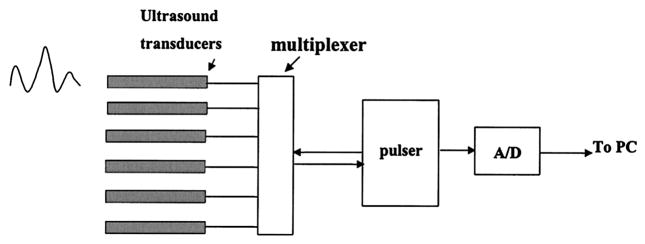
Ultrasound data-acquisition system. The pulser is used to generate high-voltage pulses that are used to excite the selected ultrasound transducer. The returned signals are received by the selected transducer and are sampled by the A/D converter.

C. Computation Procedures

1. Computation Procedures of Experimental Data

To study the relationship between the total number of source–detector pairs and distributions of reconstructed optical absorption coefficients, we started from the dense array with a total of 28 sources and 13 detectors (see Fig. 2) and gradually reduced this number to generate sparse arrays with 24 × 13 (24 sources and 13 detectors), 20 × 13, 28 × 9, 24 × 9, 16 × 13, 20 × 9, 12 × 13, 16 × 9, 28 × 5, 24 × 5, 12 × 9, 20 × 5, 16 × 5, and 12 × 5 source–detector pairs, respectively. Each sparse array was a subset of the dense array, and its probe area was the same as the dense array. For each sparse array configuration, we compared the reconstructed optical imaging parameters measured from the dense array with those from the sparse arrays. The parameters include the maximum values of reconstructed μ̂_a at different layers and their spatial locations, spatial resolution and artifact level of the μ̂_a image, and target depth distribution. Targets of different absorption contrasts were located at different positions inside the Intralipid. For each target case, one set of measurements with the dense array was obtained, and subsets of the measurements were used as sparse array measurements. In all experiments, the background Intralipid concentration was approximately 0.6%, and μ_s′ was experimentally determined from curve fitting results. Currently, we did not reconstruct target μ_s′, and we used the common μ_s′ for both the background and the target.

The total number of iterations or stopping criterion was difficult to determine for experimental data. Ideally, the iteration should stop when the object function [see Eq. (11)] or the error performance surface reaches the noise floor. However, the system noise, particularly coherent noise, was difficult to estimate. In general, we found that the reconstructed values were closer to true values when the object function reached approximately 5–15% of the initial value (total energy in the measurements). However, this criterion was applicable only to reconstructions with total source–detector pairs closer to the dense array case. Therefore we used this criterion for the dense array reconstruction and used the same iteration number obtained from the dense array for the sparse arrays. Thus the iteration number is normalized to the dense array case.

2. Computation Procedures of Simulation

Simulations were performed to assist the understanding of the random noise on the reconstructed absorption coefficient. In simulations, Gaussian noise with different standard deviations proportional to the average value of each forward data set was added to the forward measurements. Typically, 0.5%, 1.5%, and 2.0% of the average value of each forward data set were used as standard deviations to generate noise. In simulations, the target μ_a was changed to different contrast values, and target μ_s′ was kept the same as the background. The background μ_a and μ_s′ were 0.02 and 6 cm⁻¹, respectively.

The stopping criterion used in the simulations was based on the noise level of the object function. Considering that the object function fluctuates within one standard deviation σ around the mean E when the iteration number is large, we can use E + σ as a stopping criterion, i.e., the iteration will stop if the object function is less than E + σ. When the linear perturbation is assumed, E can be approximated as ${\mathrm{\sum }}_j^{N}n{(j)}^2$ and σ as ${\mathrm{\sum }}_j^N{[2n{(j)}^4]}^{1/2}$, where N is the total number of source–detector pairs and n(j) is the generated random noise with a standard deviation proportional to the specified percentage of the mean of the forward data set.

D. Testing Targets

Spherical testing targets of ~1 cm in diameter were made of acrylamide gel.¹⁶ The acrylamide powder was dissolved in distilled water, and 20% concentration of Intralipid was added to the acrylamide solution to dilute the solution to a 0.6% Intralipid concentration (μ_s′ = 6 cm⁻¹). India ink was added to the solution to produce target μ_a of different values. Acoustic scattering particles of 200 μm in diameter were added to the solution before polymerization. Components of ammonium persulfate and tetramethylethylenediamine (known as TE-MED) were added to the solution to produce polymerization.

4. Results of a High-Contrast Target Case

A. Experimental Results of a Dense Array

Figure 6(a) is an experimental image of a high-contrast target (μ_a = 0.25 cm⁻¹) located in the Intralipid background (μ_s′ = 6 cm⁻¹). The target was a 1-cm-diameter sphere and its center was located at (x = 0, y = 0, z = 3.0 cm), where x and y were the spatial coordinates and z was the propagation depth. The target depth was well controlled by use of ultrasound pulse-echo signals, and the error was less than 1 mm. The 3-D images were reconstructed from the measurements made with the dense array, and the image shown was obtained at target layer 3. The centers of the imaging voxels in z are 1, 2, 3, and 4 cm for layers 1, 2, 3, and 4, respectively. The measured maximum value of the image lobe [μ̂_a(max)] was 0.233 cm⁻¹, which was a close estimate of the target μ_a. The measured spatial location of μ̂_a(max) was (x = 0.5 cm, y = 0.0 cm), which agreed reasonably well with the true target location. The spatial resolution can be estimated from the −6-dB contour plot of Fig. 6(a), which is shown in Fig. 6(b). The outer contour is −6dB from the μ̂_a(max), and the contour spacing is 1 dB. The width of the image lobe measured at the −6 dB-level corresponds to a full width at half-maximum (FWHM), which is commonly used to estimate resolution. The measured widths of longer and shorter axes were 1.01 and 1.60 cm, respectively, and the geometric mean was 1.27 cm, which was used to represent the −6-dB beam width. The contrast resolution can be estimated from the peak artifact level, and no artifact was observed in the image. The target depth can be assessed from the images obtained from other nontarget layers. Figure 6(c) is the image obtained at nontarget layer 4, and an image lobe of μ̂_a(max) = 0.138 cm⁻¹ was observed. The spatial location of μ̂_a(max) was (x = 0.0, y = 0.0), which agreed well with the true target location. No distinct lobes were observed at nontarget layers 1 and 2, which indicates that the error in the target depth estimated from 3-D images was approximately 1 cm. Because the error in the true target depth was less than 1 mm, this 1-cm error was due largely to the depth uncertainty of diffusive waves.

Fig. 6.

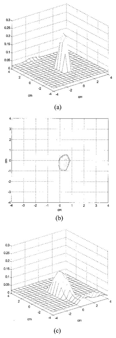
Experimental 3-D images of μ̂_a reconstructed with a total of 28 × 13 = 364 source–detector pairs at 2437 iterations. The target (μ_a = 0.25 cm⁻¹) was located at (x = 0, y = 0, z = 3.0 cm) inside the Intralipid background. (a) Reconstructed μ̂_a at target layer 3. The horizontal axes represent spatial x and y coordinates in centimeters, and the vertical axis is the μ̂_a. The measured maximum value of the image lobe [μ̂_a(max)] was 0.233 cm⁻¹, and its location was (x = 0.5, y = 0.0). No image artifacts were observed. (b) −6-dB contour plot of (a). The outer contour is −6 dB from the μ̂_a(max), and the contour spacing is 1 dB. The measured −6-dB beam width was 1.27 cm. (c) Reconstructed μ̂_a at nontarget layer 4. An image lobe of strength 0.138 cm⁻¹ and spatial location of (x = 0.0, y = 0.0) was observed.

B. Simulation Results of a Dense Array

Our simulations support the experimental results. Figure 7 shows simulation results obtained with the dense array. A simulated 1-cm-diameter absorber (μ_a = 0.25 cm⁻¹) was located at (x = 0, y = 0, z = 3 cm) inside a homogeneous scattering background (μ_s′ = 6 cm⁻¹). We added 0.5% Gaussian noise to the forward data generated from the analytic solution. Images obtained at nontarget layer 2, target layer 3, and nontarget layer 4 are shown in Fig. 7(a), Fig. (b), and 7(c), respectively. No target was found at layer 2, and the target of strengths 0.248 and 0.190 cm⁻¹ appeared at layers 3 and 4, respectively. However, when the noise level in the forward data was increased to 1.0%, the target of strength μ̂_a(max) = 0.028 cm⁻¹ appeared at nontarget layer 2 [Fig. 7(d)] as well as target layer 3 [μ̂_a(max) = 0.163 cm⁻¹] and nontarget layer 4 [μ̂_a(max) = 0.111 cm⁻¹]. This suggests that measurement noise is an important parameter to affect the target depth estimate.

Fig. 7.

Simulated 3-D images of μ̂_a reconstructed with a total of 28 × 13 = 364 source–detector pairs. The target (μ_a = 0.25 cm⁻¹) was located at (x = 0, y = 0, z = 3.0 cm) inside the Intralipid background. (a) Reconstructed μ̂_a at nontarget layer 2 (simulation, 0.5% noise). No image lobe was observed. (b) Reconstructed μ̂_a at target layer 3 (simulation, 0.5% noise). The target of strength μ̂_a(max) = 0.248 cm⁻¹ and the spatial location (0.0, 0.0) was observed. (c) Reconstructed μ̂_a at nontarget layer 4 (simulation, 0.5% noise). The target of strength 0.190 cm⁻¹ and location (x = 0.0, y = 0.0) was observed. (d). Reconstructed μ̂_a at non-target layer 2 with 1.0% noise. The target of 0.028 cm⁻¹ was observed. Note that the scale of (d) is different from (a)–(c).

C. Experimental Results of a Dense Array with Ultrasound Assistance

From ultrasound we obtained the target depth as well as the target boundary information. Figure 8(a) shows the received pulse-echo signals (from a depth of 2.3–3.5 cm) obtained from the six ultrasound transducers (see Fig. 2). The spatial dimension covered by the six transducers is 2.4 cm. The front surface of the target was indicated clearly by the returned pulses shown by two arrows, and the back surface was seen through the reflection of a soft plastic plate. The reflected signals of the back surface are also shown by arrows. The plate was used to hold the target and was transparent to light. The measured depth of the target front surface was 2.44 cm and the back surface was 3.43 cm. The distance between the peaks of front reflection and backreflection was 0.993 cm, which corresponded to the target size. With the assistance of target depth, we reconstructed the absorption image at the target layer only. Figure 8(b) is the reconstructed μ̂_a obtained from the dense array measurements. A total of 216 iterations were used to obtain μ̂_a(max) = 0.245 cm⁻¹, and the reconstruction was approximately ten times faster than that without the depth information. The spatial resolution was approximately the same as Fig. 6(a), and the −6-dB beam width was 1.31 cm. The contrast resolution was 5 dB poorer because the measurement noise was lumped to single-layer reconstruction instead of being distributed to four layers.

Fig. 8.

(a) Ultrasound pulse-echo signals or A-scan lines obtained from six transducers. The abscissa is the propagation depth in millimeters. From reflected signals, the measured depth of the target front surface is 2.44 cm, and the back surface is 3.43 cm. The center of the target is ~3 cm. The total length of the signal corresponds to 1.2 cm in depth, and the measured distance between the front and the back surfaces is 0.993 cm. The spatial dimension covered by the transducers is 2.4 cm. (b) An image of the high-contrast target reconstructed at a target layer when we used only a priori target depth information provided by ultrasound. The reconstructed μ̂_a(max) reached 0.245 cm⁻¹ at 216 iterations.

D. Experimental Results of a Sparse Array

The imaging quality of sparse arrays decreased. Figure 9(a) is an experimental image at target layer 3 obtained from the 16 × 5 sparse array. The sparse array measurements used were a subset of the dense array measurements. The measured μ̂_a(max) was 0.107 cm⁻¹, which was 43% of the true value. The −6-dB beam width was 2.55 cm, which was 200% broader than that of the dense array. Edge artifacts were observed and are best seen from Fig. 9(b), which is the −12-dB contour plot of Fig. 9(a). The outer contour is −12 dB, and the spacing is 2 dB. The peak artifact level is −10 dB from the μ̂_a(max). The reconstructed μ̂_a can be increased if the iteration is significantly increased. The iteration number used to obtain Fig. 9(a) was 2478, which was the same as that used to obtain Fig. 6. When the iteration number was increased to 10,000 for the sparse array case, the reconstructed μ̂_a(max) reached 0.264 cm⁻¹, which was close to the true target μ_a. However, the image artifact level was increased too [see Fig. 9(c)], and the ratio of the peak artifact to μ̂_a(max) was 2 dB higher than that shown in Fig. 9(a). In addition, the background noise fluctuation of nontarget layers 1 and 2 was increased. The noise fluctuation can be estimated from the standard deviations of reconstructed μ̂_a at nontarget layers 1 and 2. At 2478 iterations, the averages and the standard deviations of μ̂_a were 0.0233 (±0.0028) and 0.0202 cm⁻¹ (±0.0022 cm⁻¹) for nontarget layers 1 and 2, respectively, and these values were 0.0244 (±0.0078) and 0.0208 cm⁻¹ (±0.0073 cm⁻¹) at 10,000 iterations.

Fig. 9.

Experimental images at target layer 3 reconstructed with a total of 16 × 5 = 80 source–detector pairs. (a) Reconstructed μ̂_a at target layer 3 with 2478 iterations. The measured μ̂_a(max) was 0.107 cm⁻¹, which was 43% of the true value, and the spatial location of μ̂_a(max) was (x = 0.5, y = −0.5). The measured peak image artifact level was −10 dB below the peak of the main image lobe. (b) −12-dB contour plot of (a). The outer contour is −12 dB, and the contour spacing is 2 dB. The measured −6-dB beam width was 2.55 cm, which was 200% broader than that of the dense array. (c) Reconstructed μ̂_a at target layer 3 with 10,000 iterations. The measured μ̂_a(max) reached 0.264 cm⁻¹, and the peak artifact level was increased by 2 dB as well. (d) Reconstructed μ̂_a at the target layer with only a priori target depth information provided by ultrasound. μ̂_a(max) = 0.173 cm⁻¹ at 216 iterations.

The measured maximum values of the image lobes or target strengths at the target layer and nontarget layer 4 continuously grew with each iteration, even though the reconstructed values at the target layer were close to the true value. This problem was mentioned in the literature,¹¹ but was not explained well. It is largely related to use of nonlinear constrains on Δμ_a in Eq. (10), particularly the choice of α. When α is close to 1, the reconstruction converges fast, and the target strength increases little after a certain number of iterations. When α is close to 0, the reconstruction converges slowly, and the target strength grows continuously. However, when the measurement signal-to-noise ratio (SNR) is not high, for example, in sparse array or low-contrast cases, the choice of α ≈ 1 can cause unstable reconstruction. In some cases, the reconstructed images can jump from one set of μ̂_a to another, which causes the object function to increase suddenly and reduce again. This is related to the underdetermined nature of Eq. (10), i.e., the unknowns are far more than the measurements. In some cases the reconstructed images have multiple lobes of similar strengths, which indicate that the reconstruction does not converge at all. In all cases, the image background fluctuations were large compared with the fluctuations when a smaller α was used. We found that α between 0.1 and 0.4 can provide stable reconstruction, and we used α ≈ 0.1 for all experiments.

Another factor that accounts for the slow increase in the reconstructed value is use of linear perturbation to approximate the measurements that contain all higher-order perturbations. The minimization procedure [Eq. (11)] blindly minimizes the difference between the measurements and their linear approximation WΔμ_a and therefore reconstructs higher and higher Δμ_a if the iteration continues.

The target depth estimate was poorer than that of the dense array because of the lower SNR of the sparse array measurements. Similar to the dense array case, a target of strength μ̂_a(max) = 0.072 cm⁻¹ and location (x = 0.5, y = 0.0) was observed at non-target layer 4. In addition, a target of strength μ̂_a(max) = 0.0348 cm⁻¹ and location (x = 0.5, y = −0.5) was observed at nontarget layer 2. However, the target mass, which was approximately the volume underneath the image lobe, was much smaller than that obtained at layers 3 and 4, and the target at layer 2 was buried in the background noise.

Figure 9(d) is the reconstructed μ̂_a at the target layer from only the sparse array measurements. A total of 216 iteration steps were used to obtain μ̂_a(max) = 0.173 cm⁻¹, and the reconstruction was approximately 50 times faster than that without the depth information. The measured −6-dB beam width was 1.49 cm, which was approximately the same as Fig. 9(c) but was improved 42% from Fig. 9(a). The contrast resolution was 2 dB worse for the same reason discussed above.

E. Simulation and Experimental Results of Reconstructed μ̂_a(max) versus Total Number of Source–Detector Pairs

To understand the effects of random noise on the performance of the reconstruction, we performed simulations for each array configuration. Gaussian noise of 0.5%, 1.0%, 1.5%, and 2.0% were added to each forward data set generated from the analytic solution [see Eq. (3)]. The center of a simulated 1-cm-diameter spherical target (μ_a = 0.25 cm⁻¹) was located at (x = 0, y = 0, z = 3.0 cm). Reconstructed images at different noise levels were obtained for each array configuration, and the peak values of image lobes [μ̂_a(max)] at target layer 3 were measured. Figure 10(a) shows simulation and experimental results of reconstructed μ̂_a(max) versus the total number of source– detector pairs. Two dashed curves are the fitting results of simulated data points with 0.5% (upper) and 2.0% (lower) noise. The dashed curve in the middle is the fitting result of experimental points plotted with circles. Second-order polynomials were used for all curve fittings. The reduction of the reconstructed μ̂_a(max) was significant when the noise level went up in the simulated data. Because the SNR of experimental data was decreased when the total number of source– detector pairs was reduced, the data were scattered around the 0.5% noise curve when the total pairs were large and were distributed around the 2.0% noise curve (values were 60% less than that obtained from the dense array) when the total pairs were reduced to less than 140. However, because our experimental system has both coherent and random noise, simulations based on random noise can only qualitatively explain the noise effect on the experimental data.

Fig. 10.

μ̂_a(max) versus the total number of source–detector pairs. The center of the target (μ_a= 0.25 cm⁻¹) was located at (x = 0.0, y = 0.0, z = 3.0 cm) in computer simulations and experiments. (a) Curves were obtained at the target layer. Two dashed curves (upper and lower) are the curve-fitting results of simulation data points obtained with 0.5% and 2.0% noise added to the forward data, respectively. The experimental data are plotted with circles, and the dashed curve in the middle is the fitting result of the experimental points. (b) The measured target strength (circles) and the curve-fitting result (lower curve). The measured target strength (stars) was reconstructed at the target layer only by use of a priori depth information and the curve fitting result (upper curve).

Figure 10(b) shows the experimental results of reconstructed μ̂_a(max) versus the total number of source–detector pairs obtained from 3-D imaging (circles) and ultrasound-assisted imaging (stars). The upper curve is the fitting result of the circles, and the lower curve is the result of the stars. In both cases, the reconstructed values were decreased when the total number of pairs was reduced. However, the reconstructed values were more accurate when the target depth information was available, and the improvement on average was 15%. The improvement was more dramatic when the total pairs were less.

For sparse arrays with total source– detector pairs less than 140, the reconstructed μ̂_a(max) could be increased if the iterations were significantly increased. However, the image artifact level of the target layer and the noise level of the nontarget layers were increased too. With the assistance of simulations, we offer the following explanations to the increased image artifact and noise level problem. In simulations, the iteration was stopped when the TLS error between the measurement and the linear approximation reached the noise floor, which was

$$E+\sigma =\sum _j^{N}n{(j)}^2+\sum _j^N{[2n{(j)}^4]}^{1/2},$$

where n(j) was the generated random noise with the standard deviation proportional to a certain percent of the mean of the forward data set for each array configuration. When the object function reached the noise floor, the gradient

$$\nabla g=\frac{-2{(U_{\text{sd}}-W\mathrm{\Delta }{\mu }_a)}^T(W)}{\mathrm{\Delta }{{\mu }_a}^T\mathrm{\Delta }{\mu }_a+1}-\frac{-2{(U_{\text{sc}}-W\mathrm{\Delta }{\mu }_a)}^T(U_{\text{sd}}-W\mathrm{\Delta }{\mu }_a)(\mathrm{\Delta }{\mu }_a)}{{(\mathrm{\Delta }{{\mu }_a}^T\mathrm{\Delta }{\mu }_a+1)}^2}$$

can be approximated as

$$\nabla g\approx \frac{-2{(N)}^T(W)}{\mathrm{\Delta }{{\mu }_a}^T\mathrm{\Delta }{\mu }_a+1}-\frac{-2{(N)}^T(N)(\mathrm{\Delta }{\mu }_a)}{{(\mathrm{\Delta }{{\mu }_a}^T\mathrm{\Delta }{\mu }_a+1)}^2},$$

where N is the noise vector. Therefore the search procedure of Eq. (11) is more random and noisy. Because Δμ_a(new) = Δμ_a(old) + β∇g, the Δμ_a updating is more random and noisy. β is proportional to the square of the gradient. Continuous iteration when the object function has reached the noise floor may destroy the convergence of the reconstruction. We found that when the SNR of the data is high, for example, high-contrast cases, continuous iteration in general increases reconstructed μ_a and sidelobes. However, when the SNR of the data is low, for example, low-contrast cases, continuous iteration does not increase the reconstructed μ_a, but destroys the convergence of the reconstruction [see Fig. 12(c) below].

Fig. 12.

Experimental images of μ̂_a at target layer 3 reconstructed from a total of 24 × 5 = 120 source–detector pairs. (a) Reconstructed μ̂_a at target layer 3 with 510 iterations. The measured μ̂_a(max) was 0.049 cm⁻¹, which was 49% of the true target μ_a, and its location was (x = 0.5, y=−1.0), which was displaced from the true target location by 1.11 cm. Image artifacts were observed, and the peak was −3 dB from the μ̂_a(max). (b) −6-dB contour plot of (a). (c) Reconstructed μ̂_a at target layer 3 with 1500 iterations. The peak artifact was 5 dB higher than the image lobe. (d) Reconstructed μ̂_a at target layer 3 (56 iterations) with only a priori target depth information provided by ultrasound. The measured μ̂_a(max) was 0.074 cm⁻¹, and its location was (x = 0.5, y = −0.5). Image artifacts were observed, and the peak was −5 dB from the μ̂_a(max).

F. Experimental Results of Imaging Parameters Versus Total Number of Source–Detector Pairs

The imaging parameters measured from different array configurations are listed in Table 1. Listed first are the measured parameters at target layer 3. These parameters are a −6-dB beam width of the image lobe, the peak sidelobe level, μ̂_a(max), and the distance in the x–y plane between the location of μ̂_a(max) and the true target location. Next are the same parameters measured at nontarget layer 4. The increase in beam width was negligible for the arrays with more than 140 source–detector pairs and was 100% broader for the sparse arrays with total pairs less than this number. The sidelobe level was progressively increased when the total pairs were reduced. At nontarget layer 4, when the total pairs were reduced to less than 140, the measured image lobes were broad and no sidelobes were seen. The agreement between the measured μ̂_a(max) location and the true target location is good for all the array configurations, which suggests that this parameter is not sensitive to the total number of source–detector pairs in high-contrast cases. Table 1 next lists the strength of the target measured at nontarget layer 2 and its spatial location. Because the SNR of the sparse array measurement was lower, the target appeared at layer 2 when total pairs were less than 180. However, in all cases, the target mass measured at this layer was much smaller than that obtained at the target layer and nontarget layer 4. Finally, Table 1 lists the measured imaging parameters when the target depth was available to optical reconstruction. Compared with parameters obtained from optical imaging only, the −6-dB beam width was improved by 24% on average, and the reconstruction speed was approximately 10 times faster; however, the sidelobe was 3 dB worse.

Table 1.

Imaging Parameters Measured with Different Array Configurations: High-Contrast Target Case (μ_a = 0.25 cm⁻¹)

Parameter	Total Pairs
	28 × 13	24 × 13	20 × 13	28 × 9	24 × 9	16 × 13	20 × 9	12 × 13	16 × 9	28 × 5	24 × 5	12 × 9	20 × 5	16 × 5	12 × 5
Target layer 3 (2437 iterations)
−6-dB beam width (cm)	1.27	1.42	1.65	1.67	1.70	1.44	1.78	1.39	1.55	2.45	2.34	1.69	2.50	2.55	3.09
Peak sidelobe (dB)	−18	−13	−12	−14	−13	−16	−12	−13	−11	−12	−11	−10	−11	−10	−8
μ̂a(max) (cm−1)	0.23	0.23	0.17	0.17	0.16	0.18	0.16	0.19	0.17	0.12	0.12	0.15	0.12	0.11	0.06
|μ̂a(max) −(0,0)| (cm)	0.5	0.7	0.7	0.5	0.5	0.7	0.5	0.7	0.7	0.5	0.5	0.7	0.5	0.7	0.7
Nontarget layer 4 (2437 iterations)
−6-dB beam width (cm)	2.10	2.11	2.48	2.40	2.52	2.26	2.59	2.40	2.54	4.35	4.10	2.63	3.93	4.51	5.36
Peak sidelobe (dB)	−8	−9	−17	−14	−13	−19	−12	−13	−12
μ̂a(max) (cm−1)	0.14	0.14	0.12	0.11	0.11	0.14	0.11	0.14	0.13	0.06	0.07	0.12	0.06	0.07	0.07
|μ̂a(max) − (0,0)| (cm)	0.0	0.5	0.0	0.7	0.7	0.5	0.7	0.0	0.7	0.5	0.5	0.7	0.5	0.5	0.5
Nontarget layer 2 (2437 iterations)
μ̂a(max) (cm−1)	0.00	0.00	0.00	0.00	0.00	0.00	0.043	0.024	0.047	0.026	0.043	0.048	0.032	0.035	0.038
|μ̂a(max) − (0,0)| (cm)							1.12	0.70	1.12	0.70	1.00	1.12	0.70	0.70	0.5
Target layer only (216 iterations)
−6-dB beam width (cm)	1.31	1.40	1.68	1.61	1.55	1.57	1.50	1.41	1.20	1.71	1.48	1.45	1.77	1.49	1.75
Peak sidelobe (dB)	−12	−12	−12	−9	−8	−12	−7	−9	−7	−8	−8	−6	−8	−8	−8
μ̂a(max) (cm−1)	0.25	0.23	0.19	0.18	0.19	0.19	0.24	0.20	0.22	0.16	0.16	0.20	0.15	0.17	0.15
|μ̂a(max) − (0,0)| (cm)	0.5	0.5	0.5	0.5	0.5	0.5	0.5	0.5	0.5	0.5	0.5	0.5	0.5	0.5	0.5

Note: Italicized entries are 100% broader than the dense array beam width.

5. Results of a Lower-Contrast Target Case

A. Experimental Results of a Dense Array

To study the effects of target contrast on the quality of the reconstructed image for each array configuration, we conducted a set of experiments with a lower-contrast target (μ_a = 0.10 cm⁻¹) embedded in the Intralipid. The center of the target was located at (x = 0, y = 0, z = 2.5 cm). The centers of the imaging voxels in z were 0.5, 1.5, 2.5, and 3.5 cm for layers 1, 2, 3, and 4, respectively. Figure 11 shows the images of the lower-contrast target obtained at target layer 3 [Fig. 11(a)] and deeper nontarget layer 4 [Fig. 11(b)]. The images were reconstructed from the measurements made with the dense array. At target layer 3, the measured μ̂_a(max) was 0.063 cm⁻¹, which was approximately 63% of the target μ_a. The measured spatial location of μ̂_a(max) was (x = 0.0, y = −0.5), which agreed reasonably well with the true target location. The measured −6-dB beam width was 1.83 cm, which was 144% times broader than the beam width of the high-contrast case. Edge artifacts were observed, and the peak level was −7 dB from the μ̂_a(max). At non-target layer 4, the measured μ̂_a(max) was 0.0871 cm⁻¹, which was even higher than that measured at the target layer. Because the SNR of the data was lower than the high-contrast case, the target depth estimate was poorer. A target of μ̂_a(max) = 0.0543 cm⁻¹ located at (x = 0, y = −0.5) was observed at nontarget layer 2, and its mass was much smaller than that obtained at the target layer and nontarget layer 4.

Fig. 11.

Experimental images of μ̂_a reconstructed from a total of 28×13=364 source–detector pairs. The target (μ_a=0.10 cm⁻¹) was located at (x = 0, y = 0, z = 2.5 cm) inside the Intralipid background. (a) Reconstructed μ̂_a at target layer 3. The measured μ̂_a(max) was 0.063 cm⁻¹ at 510 iterations, and its location was (x = 0.0, y = −0.5). Edge artifacts were observed and the peak level was −7 dB from the μ̂_a(max). (b) Reconstructed μ̂_a at non-target layer 4. The measured μ̂_a(max) was 0.0871 cm⁻¹ at 510 iterations, and its location was (x = 0, y = 0). (c) Reconstructed μ̂_a at the target layer when only the target depth information provided by ultrasound was used. μ̂_a(max) = 0.107 cm⁻¹ at 56 iterations.

Figure 11(c) is the reconstructed μ̂_a at the target layer from only the dense array measurements. A total of 56 iterations were used to obtain μ̂_a(max) = 0.107 cm⁻¹, and the reconstruction was approximately ten times faster than that without the depth information. The spatial resolution was 8% better than that obtained from Fig. 11(a), and the −6-dB beam width was 1.67 cm. The contrast resolution was 2 dB worse.

B. Experimental Results of a Sparse Array

The imaging quality of sparse arrays decreased. Figure 12(a) is an image of the same target (μ_a = 0.10 cm⁻¹) reconstructed from measurements made with the 24 × 5 sparse array. The measured μ̂_a(max) was 0.049 cm⁻¹, which was 49% of the true value. The −6-dB contour plot is shown in Fig. 12(b). The measured spatial location of μ̂_a(max) was (x = 0.5, y = −1.0), which was displaced from the true target location by 1.11 cm in radius. The measured −6-dB beam width was 2.98 cm, which was 163% broader than that measured from the dense array. Sidelobes were abundant, and the peak value was −3 dB below the peak of the image lobe. These sidelobes would produce false targets in the image if no a priori information about the target locations were given.

In this case, continuous iteration did not increase the target strength but increased the sidelobe strength. Figure 12(a) was obtained at 510 iterations, whereas Fig. 12(c) was obtained at 1500 iterations. After approximately three times more iterations, the peak of the artifact was 5 dB higher than the peak of the image lobe. The target depth estimated from 3-D images was worse at 1500 iterations than that at the 510 iterations. The measured target strengths at nontarget layer 2 were 0.064 and 0.1661 cm⁻¹ at 510 and 1500 iterations, respectively, and the strengths at nontarget layer 4 were 0.0597 and 0.1087 cm⁻¹, respectively. In addition, the background noise fluctuation or standard deviation measured at nontarget layer 1 was increased with the iterations. The mean and the standard deviation at 510 iterations were 0.024 and 0.0041 cm⁻¹, whereas these values at 1500 iterations were 0.0267 and 0.0104 cm⁻¹.

As shown in Fig. 12(d), the reconstructed image improved a lot when the target depth was given. The maximum strength was 0.074 cm⁻¹, and its location was (0.5, −0.5). The −6-dB beam width was 2.63 cm, which was 12% better than that obtained from Fig. 12(a). The sidelobe was −6 dB from the peak, which was improved by 3 dB compared with Fig. 12(a).

C. Experimental Results of Reconstructed μ̂_a(max) versus Total Number of Source–Detector Pairs

With the iteration number normalized to the dense array case, we measured target strengths at target layer 3 and nontarget layer 4 for all sparse array configurations. Figure 13 shows the experimental data points (circles) of measured μ̂_a(max) versus the total number of source–detector pairs obtained at target layer 3 [Fig. 13(a)] and nontarget layer 4 [Fig. 13(b)]. The two curves were the fitting results of experimental points when we used second-order polynomials. In both layers, the μ̂_a(max) values were decreased when the total number of source–detector pairs was reduced. The reconstructed target strengths were reduced to less than 60% when the total pairs were less than 156 and 140 for target layer 3 and nontarget layer 4, respectively. The ultrasound-assisted reconstruction results are shown in Fig. 13(a) (stars), and the average reconstructed μ̂_a(max) for all array configurations was 0.085 cm⁻¹. Compared with the average of 0.055 cm⁻¹ obtained from optical imaging only at the target layer, a 30% improvement was achieved.

Fig. 13.

Low-contrast target case. (a) Reconstructed μ̂_a(max) versus total source–detector pairs with the target depth available (stars) and the curve-fitting results (upper curve). Reconstructed μ̂_a(max) versus total source–detector pairs measured at target layer (circles) and the curve-fitting results (lower curve) and (b) at deeper nontarget layer 4.

D. Experimental Results of Imaging Parameters versus Total Number of Source–Detector Pairs

The measured imaging parameters obtained from different array configurations are listed in Table 2. Similar to Table 1, listed are the measured parameters at target layer 3 and nontarget layer 4. The increase in beam width at the target layer was negligible for the arrays with more than 156 source-detector pairs and was more than 50% for the sparse arrays with total pairs less than this number. The sidelobes were progressively worse when the total pairs were reduced. At the target layer, the distance between the μ̂_a(max) location and the true target location was more than 1 cm for the arrays with total pairs less than 140. Table 2 then lists the measured peak image lobe at nontarget layer 2 and its location. The target appeared at nontarget layer 2 in all array configurations because of the lower SNR of the data. However, the target mass observed at this layer was much smaller than that at layers 3 and 4 in all cases. The last row in Table 2 shows the measured imaging parameters when the target depth was available to optical reconstruction. Compared with parameters obtained from optical imaging only, the −6-dB beam width was improved by 41% on average, and the reconstruction speed was approximately ten times faster; however, the sidelobe was 1 dB worse.

Table 2.

Imaging Parameters Measured with Different Array Configurations: Lower-Contrast Target Case (μ_a = 0.10 cm⁻¹)

Parameter	Total Pairs
	28 × 13	24 × 13	20 × 13	28 × 9	24 × 9	16 × 13	20 × 9	12 × 13	16 × 9	28 × 5	24 × 5	12 × 9	20 × 5	16 × 5	12 × 5
Target layer 3 (510 iterations)
−6-dB beam width (cm)	1.83	1.98	2.02	2.24	1.86	2.09	2.42	2.73	3.07	3.07	2.98	4.10	3.57	4.23	3.07
Peak sidelobe (dB)	−6	−6	−7	−4	−3	−5	−2	−6	−3	−4	−3	−1	−3	−2	−2
μ̂a(max) (cm−1)	0.06	0.06	0.07	0.06	0.07	0.07	0.06	0.05	0.06	0.05	0.05	0.04	0.05	0.05	0.04
|μ̂a(max) − (0,0)| (cm)	0.5	0.5	0.7	1.0	0.7	0.7	0.7	0.7	0.7	1.11	1.11	1.11	1.0	1.0	1.58
Nontarget layer 4 (510 iterations)
−6-dB beam width (cm)	3.36	3.42	3.31	4.81	3.08	3.28	4.69	4.20	5.49	5.57	5.15	4.88	6.62	8.49	8.81
Peak sidelobe (dB)	−8	−9	−8	−6	−7	−7	−5
μ̂a(max) (cm−1)	0.09	0.09	0.08	0.07	0.08	0.08	0.07	0.07	0.07	0.05	0.06	0.06	0.05	0.06	0.05
|μ̂a(max) − (0,0)| (cm)	0.0	0.0	0.5	0.7	0.5	0.5	0.5	0.5	0.5	0.5	0.5	1.11	0.5	0.5	0.5
Nontarget layer 2 (510 iterations)
μ̂a(max) (cm−1)	0.062	0.058	0.054	0.048	0.051	0.049	0.047	0.046	0.047	0.054	0.064	0.034	0.060	0.064	0.049
|μ̂a(max) − (0,0)| (cm)	0.70	0.70	0.70	0.5	0.70	1.12	0.5	1.12	0.0	0.70	0.0	0.50	0.0	0.0	0.70
Target layer only (56 iterations)
−6-dB beam width (cm)	1.67	2.43	2.35	1.72	2.10	1.93	1.56	3.12	2.37	2.12	2.63	1.12	1.84	1.86	3.30
Peak sidelobe (dB)	−4	−5	−6	−3	−3	−6	−2	−6	−4	−4	−5	−5	−4	−3	−2
μ̂a(max) (cm−1)	0.11	0.08	0.08	0.09	0.08	0.10	0.12	0.07	0.08	0.08	0.07	0.09	0.09	0.06	0.06
|μ̂a(max) − (0,0)| (cm)	0.7	0.0	0.0	0.5	0.0	0.7	0.0	0.7	0.0	0.7	0.7	1.11	0.7	0.5	0.7

Note: Italicized entries are 50% broader than the dense array beam width.

6. Discussion

In addition to the total number of source–detector pairs, the measured imaging parameters are also related to other system parameters, for example, modulation frequency and system noise. The 140-MHz modulation frequency chosen in this study is a typical frequency used by many research groups. Our system noise level, including both coherent and incoherent, is less than 10 mV peak to peak, which is sufficiently low. Therefore the results we obtained are pertinent to 3-D imaging using similar system parameters and reflection geometry.

In this study the target absorption coefficient was reconstructed from measurements. Similar studies can be done for the scattering coefficient as well. To reconstruct the scattering coefficient, we can use the scattering weight matrix derived by O’Leary¹¹ to relate the medium scattering variations with the measurements. Simultaneous reconstruction of both absorption and scattering coefficients in reflection geometry is also possible, provided that the absorption and scattering weight matrices are regulated carefully. Because the eigenvalues of the two matrices are significantly different, good regulation schemes are needed to balance the reconstructed absorption and scattering coefficients at each iteration. This subject is one of our topics for further study.

In this study the ultrasound-assisted optical reconstruction was demonstrated at a particular target layer. Similar studies can be done with multiple targets located at different layers. In the multiple target case, we can attribute measured perturbations to more layers instead of a single layer. However, the improvements in reconstructed optical properties and reconstruction speed may be less than that of the single-layer case.

Ultrasound has good imaging capability, and it can detect small lesions of a few millimeters in size. However, its specificity in cancer detection is not high as a result of overlapping characteristics of benign and malignant lesions. NIR imaging has high specificity in cancer detection; however, it suffers low resolution and lesion location uncertainty because of the diffused nature of the NIR light. The hybrid imaging that combines ultrasound imaging capability and NIR contrast has a great potential to overcome deficiencies of either method. As we reported in the paper, the target depth information can significantly improve the accuracy of the reconstructed optical absorption coefficient and reconstruction speed. In addition to use of a priori target depth information, the target spatial distribution provided by ultrasound can be used in optical reconstruction as well.¹⁵ With the localized spatial and temporal target information, the accuracy of the reconstructed optical properties and the reconstruction speed can be improved further. To demonstrate this, we need an ultrasound imaging transducer located at the middle portion of the probe. We are currently pursuing this study.^23,24

In this study the targets of different contrasts were located at the center position. We have also done studies with targets of different contrasts located at off-center positions. For an off-center target case, the effective number of source–detector pairs is less than that of the on-center target case because measurements from certain source–detector pairs do not contain much information about the target. For example, if a target is placed at (x = 2, y = 2, z = 3.0 cm), the measurements of source–detector pairs at the opposite corner of the probe contribute little to the image reconstruction. In one study, targets of high and low contrast were located at (x = 2, y = 2, z = 3.0 cm). The reconstructed maximum absorption coefficient at the target layer was related more to the total neighbor source–detector pairs. However, the maximum value at a deeper nontarget layer was related more to the total source–detector pairs and was decreased with the reduction of total pairs. Because the photons originated from distant sources and detected by distant detectors experience longer and more diffused scattering paths, they are likely to interact with the off-center target and contribute to the absorption estimate at the deeper layer. In the same study, the measured sidelobe levels were 4.5 and 2.0 dB poorer on average compared with the on-center high- and low-target cases, respectively. The beam widths were comparable to those measured from on-center cases.

7. Summary

The relationship between the total number of source-detector pairs and the imaging parameters of a reconstructed absorption coefficient was evaluated experimentally. A frequency-domain system of a 140-MHz modulation frequency was used in the experiments. Reconstruction at a selected target depth with a priori depth information provided by ultrasound was demonstrated. The results have shown that the reconstructed absorption coefficient and the spatial resolution of the absorption image were decreased when the total number of source-detector pairs was reduced. More than 160 source-detector pairs were needed to reconstruct the absorption coefficient within 60% of the true value and spatial resolution comparable to that obtained with the dense array. The contrast resolution was poorer in general because of edge artifacts and could be worse if significant larger iteration numbers are used for reconstruction. The error in target depth estimated from 3-D optical images was approximately 1 cm. With the a priori target depth information provided by ultrasound, the reconstruction can be done at a selected depth. Because the unknowns were reduced significantly, the reconstruction speed was approximately ten times faster than that without depth information. In addition, the accuracy of the reconstructed absorption coefficient was improved by 15% and 30% on average for high- and low-contrast cases, respectively. Furthermore, the measured −6-dB beam width was improved by 24% and 41% for high- and low-contrast cases, respectively. The sidelobe was 3 and 1 dB poorer for high-and low-contrast cases because the measurement noise was lumped to single-layer reconstruction instead of multiple layers.

In conclusion, ultrasound-assisted 3-D optical imaging has shown promising results to overcome the problems associated with the reconstruction by use of diffusive waves. With the target depth information provided by ultrasound, the reconstructed absorption coefficient was more accurate and the reconstruction speed was much faster.

References

- 1.Fantini S, Walker S, Franceschini M, Kaschke M, Schlag P, Moesta K. Assessment of the size, position, and optical properties of breast tumors in vivo by noninvasive optical methods. Appl Opt. 1998;37:1982–1989. doi: 10.1364/ao.37.001982. [DOI] [PubMed] [Google Scholar]
- 2.Zhou S, Chen Y, Nioka Q, Li X, Pfaff L, Cowan CM, Chance B. Portable dual-wavelength amplitude cancellation image system for the determination of human breast tumor. Optical Tomography and Spectroscopy of Tissue III. In: Chance B, Alfano R, Tromberg B, editors. Proc SPIE. Vol. 3597. 1999. pp. 571–579. [Google Scholar]
- 3.Danen RM, Wang Y, Li XD, Thayer WS, Yodh AG. Regional imager for low resolution functional imaging of the brain with diffusing near-infrared light. Photochem Photobiol. 1998;67:33–40. [PubMed] [Google Scholar]
- 4.McBride T, Pogue BW, Gerety E, Poplack S, Osterberg U, Pogue B, Paulsen K. Spectroscopic diffuse optical tomography for the quantitative assessment of hemoglobin concentration and oxygen saturation in breast tissue. Appl Opt. 1999;38:5480–5490. doi: 10.1364/ao.38.005480. [DOI] [PubMed] [Google Scholar]
- 5.Franceschini MA, Moesta KT, Fantini S, Gaida G, Gratton E, Jess H, Seeber M, Schlag PM, Kashke M. Frequency-domain techniques enhance optical mammography: initial clinical results. Proc Natl Acad Sci USA. 1997;94:6468–6473. doi: 10.1073/pnas.94.12.6468. [DOI] [PMC free article] [PubMed] [Google Scholar]
- 6.Fishkin JB, Coquoz O, Anderson ER, Brenner M, Tromberg BJ. Frequency-domain photon migration measurements of normal and malignant tissue optical properties in human subject. Appl Opt. 1997;36:10–20. doi: 10.1364/ao.36.000010. [DOI] [PubMed] [Google Scholar]
- 7.Troy TL, Page DL, Sevick-Muraca EM. Optical properties of normal and diseased breast tissues: prognosis for optical mammography. J Biomed Opt. 1996;1(3):342–355. doi: 10.1117/12.239905. [DOI] [PubMed] [Google Scholar]
- 8.Grable RJ, Rohler DP, Kla S. Optical tomography breast imaging. In: Chance B, Alfano R, editors. Optical Tomography and Spectroscopy of Tissue: Theory, Instrumentation, Model, and Human Studies II; Proc. SPIE; 1997. pp. 197–210. [Google Scholar]
- 9.Jiang H, Paulsen K, Osterberg U, Pogue B, Patterson M. Optical image reconstruction using frequency-domain data: simulations and experiments. J Opt Soc Am A. 1995;12:253–266. [Google Scholar]
- 10.Zhu W, Wang Y, Deng Y, Yao Y, Barbour R. A wavelet-based multiresolution regularized least squares reconstruction approach for optical tomography. IEEE Trans Med Imaging. 1997;16(2):210–217. doi: 10.1109/42.563666. [DOI] [PubMed] [Google Scholar]
- 11.O’Leary MA. PhD dissertation. University of Pennsylvania; Philadelphia, Pa: 1996. Imaging with diffuse photon density waves. [Google Scholar]
- 12.Li X, Durduran T, Yodh A, Chance B, Pattanayak DN. Diffraction tomography for biomedical imaging with diffuse-photon density waves. Opt Lett. 1997;22:573–575. doi: 10.1364/ol.22.000573. [DOI] [PubMed] [Google Scholar]
- 13.Matson C, Liu H. Analysis of the forward problem with diffuse photon density waves in turbid media by use of a diffraction tomography model. J Opt Soc Am A. 1999;16:455–466. [Google Scholar]
- 14.Matson C, Liu H. Backpropagation in turbid media. J Opt Soc Am A. 1999;16:1254–1265. [Google Scholar]
- 15.Zhu Q, Dunrana T, Holboke M, Ntziachristos V, Yodh A. Imager that combines near-infrared diffusive light and ultrasound. Opt Lett. 1999;24:1050–1052. doi: 10.1364/ol.24.001050. [DOI] [PubMed] [Google Scholar]
- 16.Zhu Q, Sullivan D, Chance B, Dambro T. Combined ultrasound and near infrared diffusive light imaging. IEEE Trans Ultrason Ferroelectr Freq Control. 1999;46:665–678. doi: 10.1109/58.764853. [DOI] [PubMed] [Google Scholar]
- 17.Zhu Q, Conant E, Chance B. Optical imaging as an adjunct to sonograph in differentiating benign from malignant breast lesions. J Biomed Opt. 2000;5(2):229–236. doi: 10.1117/1.429991. [DOI] [PubMed] [Google Scholar]
- 18.Jholboke M, Tromberg BJ, Li X, Shah N, Fishkin J, Kidney D, Butler J, Chance B, Yodh AG. Three-dimentional diffuse optical mammography with ultrasound localization in human subject. J Biomed Opt. 2000;5(2):237–247. doi: 10.1117/1.429992. [DOI] [PubMed] [Google Scholar]
- 19.Boas DA, O’Leary MA, Chance B, Arjun AG. Scattering of diffuse photon density waves by spherical inhomogeneities within turbid media: analytic solution and applications. Proc Natl Acad Sci USA. 1994;91:4887–4891. doi: 10.1073/pnas.91.11.4887. [DOI] [PMC free article] [PubMed] [Google Scholar]
- 20.Zhu W, Wang Y, Zhang J. Total least-squares reconstruction with wavelets for optical tomography. J Opt Soc Am A. 1998;15:2639–2650. doi: 10.1364/josaa.15.002639. [DOI] [PubMed] [Google Scholar]
- 21.Li PC, Flax W, Ebbini ES, O’Donnell M. Blocked element compensation in phased array imaging. IEEE Trans Ultrason Ferroelectr Freq Control. 1993;40:283–292. doi: 10.1109/58.251276. [DOI] [PubMed] [Google Scholar]
- 22.Golub GH. Some modified matrix eigenvalue problems. SIAM (Soc Ind Appl Math) Rev. 1973;15:318–334. [Google Scholar]
- 23.Piao D, Ding X-H, Guo P, Zhu Q. Optimal distribution of near infrared sensors for simultaneous ultrasound and NIR imaging. Biomedical Topical Meetings, Postconference Digest, Vol. 38 of OSA Trends in Optics and Photonics Series; Optical Society of America; Washington, D.C. 2000. pp. 472–474. [Google Scholar]
- 24.Guo P, Zhu Q, Piao D, Fikiet J. Combined ultrasound and NIR imager. Biomedical Topical Meetings, Postconference Digest, Vol. 38 of OSA Trends in Optics and Photonics Series; Washington, D.C: Optical Society of America; 2000. pp. 97–99. [Google Scholar]