Sparsely correlated hidden Markov models with application to genome-wide location studies

Abstract

Motivation: Multiply correlated datasets have become increasingly common in genome-wide location analysis of regulatory proteins and epigenetic modifications. Their correlation can be directly incorporated into a statistical model to capture underlying biological interactions, but such modeling quickly becomes computationally intractable.

Results: We present sparsely correlated hidden Markov models (scHMM), a novel method for performing simultaneous hidden Markov model (HMM) inference for multiple genomic datasets. In scHMM, a single HMM is assumed for each series, but the transition probability in each series depends on not only its own hidden states but also the hidden states of other related series. For each series, scHMM uses penalized regression to select a subset of the other data series and estimate their effects on the odds of each transition in the given series. Following this, hidden states are inferred using a standard forward–backward algorithm, with the transition probabilities adjusted by the model at each position, which helps retain the order of computation close to fitting independent HMMs (iHMM). Hence, scHMM is a collection of inter-dependent non-homogeneous HMMs, capable of giving a close approximation to a fully multivariate HMM fit. A simulation study shows that scHMM achieves comparable sensitivity to the multivariate HMM fit at a much lower computational cost. The method was demonstrated in the joint analysis of 39 histone modifications, CTCF and RNA polymerase II in human CD4+ T cells. scHMM reported fewer high-confidence regions than iHMM in this dataset, but scHMM could recover previously characterized histone modifications in relevant genomic regions better than iHMM. In addition, the resulting combinatorial patterns from scHMM could be better mapped to the 51 states reported by the multivariate HMM method of Ernst and Kellis.

Availability: The scHMM package can be freely downloaded from http://sourceforge.net/p/schmm/ and is recommended for use in a linux environment.

Contact: ghoshd@psu.edu or zhaohui.qin@emory.edu

Supplementary information: Supplementary data are available at Bioinformatics online.

1 INTRODUCTION

The hidden Markov model (HMM) is an important tool for learning probabilistic models of sequential data with a local correlation pattern, as exemplified in many engineering applications such as speech and handwriting recognition (Rabiner, 1989). In an HMM, it is assumed that the system has a series of unobserved (hidden) states following a Markov process. The observed data are considered as output from the hidden states and follow specific distributions. In recent years, HMMs have been successfully applied to many problems in computational molecular biology (Churchill, 1989; Krogh et al., 1994) and statistical genetics (Lander and Green, 1987). In these applications, they were used to model spatial patterns such as genomic features on the chromosomes, similar to temporal patterns in time series data.

HMM analysis is already common in genome-wide location studies. For example, the chromatin immunoprecipitation (ChIP) protocol, coupled with microarray (ChIP-chip) (Ren et al., 2000, Iyer et al., 2001) or next generation sequencing (ChIP-seq) (Johnson et al., 2007; Barski et al., 2007), is a method of choice for identifying genomic loci enriched with various histone modification marks. In ChIP-seq data, sequence reads are aligned to the target genome and data are summarized by counting the aligned reads in non-overlapping contiguous windows (e.g. 200 bp windows). Because data manifest a clear spatial correlation, an HMM is frequently used to infer the binding status of each window (Ji and Wong, 2005; Li et al., 2005; Choi et al., 2009; Qin et al., 2010), where the hidden state space consists of binding state and background state.

With the declining experimental cost, it has become increasingly common for genome-wide location analysis to be conducted on multiple regulatory proteins or epigenetic marks (Heintzman et al., 2007; Mikkelsen et al., 2007; Wang et al., 2008). Because many factors interact with each other to carry out biological processes, it is of great interest to understand the correlation among these factors as reflected in the shared binding sites or modification marks. In the context of HMM analysis with two hidden states in each series, one can formulate N separate HMMs by assuming independence between every pair of series, as illustrated in Figure 1a (referred to as iHMM hereafter). Alternatively, one can formulate a single HMM with 2^N hidden states (Fig. 1b, referred to as fullHMM), where 2^N is the number of hidden states when there are two states in each series. They represent two opposite extremes in the sense that iHMM completely ignores the correlation between series, whereas fullHMM incorporates the correlation in the multivariate model for the hidden states. Both approaches have advantages and shortcomings: iHMM may feature low statistical power, but it is computationally efficient. In contrast, fullHMM embodies the correlation directly; however, not all hidden state combinations necessarily appear in the data and it is computationally expensive, if not intractable. Practically, however, estimation of an HMM with 2^N hidden states is computationally intractable when N is large because 4^N possible transitions need to be followed.

Fig. 1.

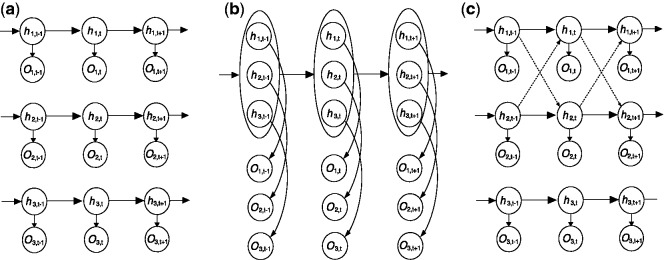
Three strategies to model multiple data series: (a) independent HMMs, (b) fully coupled HMM and (c) sparsely correlated HMMs for series data O. Associated with observed data are hidden states h, which are to be inferred. For c, the arrows in dashed lines indicate the couplings introduced to adjust the transition kernel of each series

Here we present a novel statistical model that represents a compromise of these two, termed sparsely correlated HMM (scHMM). The scHMM approach captures a small subset of non-ignorable correlations among data series to avoid modeling all pairwise correlations. This sparsity property is achieved by adopting a regularization regression strategy. Figure 1c illustrates our proposed method. The dashed-line arrows connecting the hidden states between series indicate the significant correlations captured by scHMM. For example, the hidden states at windows t − 1 and t in the first series, but not the third, are used to estimate the transition probability between windows t − 1 and t in the second series, and vice versa. Under this framework, there is no need to consider combinations of hidden states across all series (as N-tuples) as in fullHMM, and hidden states can be inferred considering just four types of transitions in each series separately (solid lines). The scHMM algorithm is able to take advantage of the interactions between correlated series to improve the inference of hidden states. Moreover, we also reduce the computational cost by iterating through N series and inferring the hidden state vectors one series a time, conditioning on the current hidden state vector estimates of all other series.

Note that the goal of scHMM is different from that of the multivariate HMM method developed by Ernst and Kellis (2010) for the analysis of combinatorial patterns of histone modification using ChIP-seq data. scHMM aims to infer the hidden states in the multiple chains simultaneously, whereas the multivariate HMM attempts to identify a small subset of representative combinatorial patterns and annotate the genome with respect to such patterns. Nevertheless, the ChIP-enriched windows identified by scHMM can be used to facilitate the multivariate HMM analysis, potentially improving the quality of genomic annotation.

2 METHODS

2.1 Overview

Suppose that data have been collected from multiple genome-wide experiments that are related to each other, for example, DNA-binding proteins that are part of a protein complex, or the same DNA-binding proteins profiled under different treatment conditions or different cell lines. Each experiment yields a data series measured across the genome. Assume that there are N series, denoted by for and , where denotes the observed datum (emission) at window t. The observed data O are associated with binary hidden states indicating the status of either true binding site (state 1) or background site (state 0). We also use and to denote the observed data and hidden states, respectively, at window t across all series. The goal of HMM analysis is the estimation of H.

As mentioned above, iHMM is a straightforward approach where each series j has an independent HMM with the two states. Standard HMM for a single data series has three components: (i) the probability mass function of the first window ; (ii) the transition kernel K_j,

where

which is constant for all windows ; and (iii) the emission and for all t. The likelihood of this model can be written as

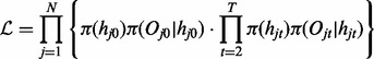(1)

Given the three components, the forward–backward algorithm can be applied to infer the hidden states quickly (Rabiner, 1989).

Although iHMM is fast and straightforward, it is unable to capture the correlation between related data series. This correlation can be explicitly incorporated in the model to increase statistical power and remove noise. The most intuitive approach is fullHMM, a single HMM with 2^N hidden state combinations and transition kernel K. The likelihood of fullHMM is

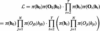Here we assume that the emission is independent of the hidden states in other series, i.e. for all j and t. Similar to iHMM, the forward–backward algorithm can be applied to infer the hidden states as well.

2.2 Sparsely correlated hidden Markov models

Although fullHMM accounts for the Markovian dynamics between hidden state combinations, not all combinations necessarily occur in the data and, more importantly, the order of computation for the forward–backward algorithm is as opposed to in iHMM. This clearly limits the applicability of fullHMM to cases with small or moderate N. When the goal of analysis is inference of hidden states in each series, fullHMM will be computationally inefficient. This motivated us to develop scHMM, a compromise between the two methods.

In the scHMM algorithm, we allow different series to be correlated as in fullHMM. At the same time, we apply two strategies, which reduce the computational cost to a level similar to that of iHMM. First, instead of considering all series simultaneously, we iteratively infer parameters by cycling through each series individually. For each individual series, inference is performed conditioning on the current hidden state vectors in all other series. Second, in each series, we assume sparsity when incorporating correlations between the current series and all other series. The correlation imposed is of the form of an inhomogeneous transition kernel. To be specific, we denote the transition kernel of scHMM for series j at window t by

which has an additional index (t) because the transition probability varies by window t. Here, we define p_jt and q_jt to incorporate the input from other series as follows:

That is, the transition probability in series j is adjusted by the hidden states in other series . Here we consider two logistic regression models in each data series:

(2)

(3)

where Equations (2) and (3) hold on windows and , respectively. In the equations, the superscripts p and c indicate ‘previous’ and ‘current’ windows, respectively. In this setup, each regression coefficient carries a straightforward interpretation. For example, the intercept term is the baseline log odds for transition in series j when all other correlated series are in the background state (state 0) at windows t − 1 and t. and are the increase in the log odds of transition in series j when previous and current windows are in binding/modification state (state 1) in series k (), respectively.

In the current form, however, the number of regression coefficients will keep growing as more series are incorporated in the analysis. To address this concern, we impose a sparsity constraint using a LASSO penalty (Tibshirani, 1996) such that

The details of the estimation procedure, including the coordinate descent algorithm by Friedman et al. (2010), are provided in the Supplementary Information.

Lastly, because our major application of interest is read count data from ChIP-seq experiments, we used a flexible class of distributions for emission, including zero-inflated mixture model for the background sites (state 0) and generalized Poisson distribution for the binding/modification sites (state 1). These distributions were previously used in the HPeak software (Qin et al., 2010).

We remark that the computational time of scHMM is significantly less than that of fullHMM. To see this, note that there are two elements in the total computation time of scHMM: one for inferring hidden states and the other for learning the regression coefficients. For the former, the complexity is no more than , where α is the additional time to compute the odds using hidden state predictors at each transition, which should be trivial unless N is very large (α should be close to 1). For the latter, the computational complexity is the time it takes to fit 2N logistic regression models with LASSO penalty in datasets with covariates and T data points, and thus this can be time-consuming in large datasets (large T) like genome-wide ChIP-seq data, and thus we randomly sample genomic regions of a sufficient size (as shown in section 4.1) and fit the model using the subset to save time. Therefore, the computation should be much more efficient than fullHMM.

3 SIMULATION STUDIES

To evaluate the performance of scHMM, we conducted simulation studies. Because typical quantitative data reported from sequencing experiments are read counts, we used Poisson distributions to generate the count data with varying signal-to-noise ratios. scHMM is applicable to a wide range of scenarios, but we considered the representative cases where scHMM is deemed beneficial. Three different models are compared side by side: iHMMs, scHMMs and fullHMM, and the performance was evaluated in terms of receiver-operating characteristic (ROC) curves (Supplementary Figs S1 and S2). Datasets were generated 10 times owing to computational time constraints in fullHMM in each simulation, and ROC curves were averaged over them.

3.1 Independent experiments

We first simulated three data series where there was no systematic correlation between series. This simulation was conducted to assess whether scHMM picks up false positives, in which case scHMM should underperform iHMM. On a dataset with 10 000 windows in 3 series, we planted mound-shaped signals (state 1), of average length 5 consecutive windows, at random positions in all series, and regarded all other windows to be in the background state (state 0). The read counts in the background state were generated from Poisson distribution with mean 5, whereas the read counts in the real binding state were generated from Poisson distribution with mean 7.5, 10 and 15. Figure 2a shows that, as expected, all three HMMs yield nearly identical ROC curves in the case of 2-fold data (Poisson mean 10 for signal), and the results were the same in 1.5- and 3-fold data as well (data not shown).

Fig. 2.

Simulation studies. Each method is represented by different symbols: squares for iHMM, circles for scHMM and triangles for fullHMM. (a) Independent case (2-fold): short-length signals were planted in random locations in three different series data. (b) One-group case (2-fold): replicate experiments where binding sites are expected to be shared in all experiment. (c) Two-group case (2-fold): two sets of three correlated series. (d) Three-group case (2-fold): three inter-dependent groups of two correlated series. In all panels, signal was simulated from Poisson (10) and background noise was simulated from Poisson (5)

3.2 Replicated ChIP experiments

We then considered the scenario of replicate experiments. We assumed that ChIP experiments for a transcription factor were repeated three times, each giving one data series. We planted signals of average length 10 windows centered at every 50th window (with 75% chance at each position), and regarded all other windows to be in the background state. Read counts were generated the same way as described above (1.5-, 2- and 3 fold). In all cases, because the mounds were planted in shared binding sites across replicates, hidden states were expected to be highly correlated between all three series. Indeed, the between-series coefficients and were mostly positive, indicating an increase in the log odds of the and transitions when other series are in binding states in the past and current positions. The ROC curves in Figure 2b clearly demonstrate that scHMM improved the sensitivity and specificity over iHMM, but not as good as fullHMM.

3.3 Groups of experiments with shared binding sites

Next we considered a more realistic scenario with six ChIP experiments. We used the same emission distributions (Poisson) for generating the simulation data as above. Here we assumed two and three groups of correlated experiments. In the two-group case, the windows containing signals were shared across the series within each group, but not between the groups. In the three-group case (each with two series), windows containing signals were mutually exclusive between the first two groups, but both groups shared such windows with the third group. As expected, the regression coefficients for the transition were positive within each group in both two- and three-group cases, but they were zero for the between-groups coefficients. For the three-group case, there were additional positive coefficients between the first and third groups and between the second and third groups, in accordance with the data generation mechanism. In both examples, the ROC curve for scHMM showed improved sensitivity over iHMM at all points, at times almost identical to that of fullHMM (Fig. 2c and d). Interestingly, fullHMM sometimes showed slightly poorer specificity compared with scHMM in some simulations because fullHMM picked up too many signals from the background regions. Moreover, even in this mini-scale data, the computational time for fullHMM was 10–15 minutes, whereas scHMM took <10 seconds, indicating a significant improvement in computational efficiency for achieving a similar ROC profile.

4 ANALYSIS OF HISTONE MODIFICATIONS IN HUMAN CD4+ T CELLS

In eukaryotic organisms, DNA is packaged into a chromatin structure by wrapping DNA around histones. It has been discovered that the cellular state is closely related to the modification patterns of the histone, or chromatin state (Bernstein et al., 2007; Kouzarides, 2007). For this reason, it is of great interest in biology to construct a genome-wide map of chromatin states in different cell types. An increasing number of studies have reported genome-wide data for multiple histone modifications using ChIP-chip (Kim et al., 2005) or ChIP-seq (Mikkelsen et al., 2007). Because multiple histone modification marks are involved in transcriptional regulation and many of them are closely related, it is highly desirable to analyze these datasets jointly; scHMM is an ideal method for such analysis. In this study, we applied scHMM to a large-scale ChIP-seq dataset, which surveyed 39 histone acetylations and methylations in the human genome, in addition to RNA polymerase II (RNA Pol II) and insulator binding protein CTCF (Barski et al., 2007; Wang et al., 2008).

4.1 Data processing and model fitting

We downloaded the raw sequence read data from the SRA database (∼243 million reads) and performed preprocessing of data, including alignment against the most recent release of the human genome (hg19) using the bowtie software (Langmead et al., 2009). Then we extracted read count data in 15.4 million 200 bp windows (contiguous non-overlapping). See Supplementary Information for details. Using the processed data, we fit iHMM and scHMM for each chromosome separately. fullHMM did not finish a single iteration in 2 days for any of the 24 chromosomes. In contrast, it took ∼20 minutes to fit scHMM for each chromosome; thus, fullHMM was excluded for further analysis. For scHMM, fitting a penalized regression for the entire data (millions of windows in 41 data series) is computationally demanding, and hence we randomly sampled 100 blocks of 500 windows (each ranging 10 kb) from each chromosome and used them to train the regression coefficients, which were later used to estimate the posterior probability (pp) of enrichment across the whole chromosome. As expected, the regression coefficients were similar across chromosomes. Overall, both iHMM and scHMM reported a various number of ChIP-enriched windows with . In both analyses, the six histone methylations H2BK5me1, H3K4me1, H3K4me3, H3K9me1, H3K36me3 and H4K20me1 were the most abundant modifications across the genome, followed by various acetylations of H3 and H4, RNA Pol II and CTCF, for which pp was above 0.9 in more than 40 000 windows. In total, scHMM reported fewer ChIP-enriched windows than iHMM (see Supplementary Table S1).

To see whether scHMM effectively incorporated the correlation, we computed two correlation matrices of the histone modifications using the estimated probabilities (pp) reported by scHMM and iHMM, respectively, and performed agglomerative hierarchical clustering on each correlation matrix. Both correlation matrices showed a large acetylation block mainly consisting of acetylation marks, suggesting that histone acetylations are more concerted than histone methylations across the genome. Both blocks contain the 17-member ‘modification backbone’ described in the original study by Wang et al. (2008). By close inspection, we found that the acetylation block generated from scHMM contained 26 marks, four more than that generated from iHMM. The four additional marks are all acetylation marks: H4K12ac, H4K16ac, H2AK9ac and H2AK5ac. The inclusion of these four marks is supported by observing the histone acetylation patterns in the transcription start site (TSS) region and across the gene bodies of 1000 highly active or silent genes reported in Wang et al. (2008). Moreover, the scHMM output showed increased correlation among closely related modifications over the iHMM output across the data. For example, in the large group of 26 modifications clustered together by scHMM (Fig. 3b), 299 pairs showed increased correlation and 26 pairs showed decreased correlation in scHMM compared with iHMM.

Fig. 3.

Correlation between 39 histone modifications (and RNA Pol II and CTCF) using the probability estimates from iHMM and scHMM

4.2 Histone modifications in actively transcribed genes

For real datasets, we cannot directly evaluate the sensitivity and specificity of the two HMM algorithms. Instead, we examined the modification patterns of well-characterized histone modifications. We learned from Wang et al. (2008) that 17 modifications in the backbone module tend to co-localize at gene promoters, and genes associated with these modifications tend to have higher expression. In particular, Koch et al. (2007) also found from the ENCODE data (The ENCODE Project Consortium, 2004) that H3K4me3, a member of the backbone module, accumulates in the promoter region of actively transcribed genes. In contrast, Bannister et al. (2005) observed that another key modification H3K36me3 peaks toward the 3′ end of actively transcribed genes. By examining whether the similar pattern holds in our genome-wide data, we can indirectly assess the sensitivity and specificity of the two methods. To this end, we first obtained the gene expression profile of the same human CD4+ T cells from Wang et al. (2009), and identified 1206 genes with the highest expression level. This number corresponds to 10% of the genes that could be mapped to the Ensembl transcripts we considered in the ChIP-seq data. We refer to these genes as ‘actively transcribed’ genes (ATGs) hereafter.

For each modification in the backbone module, we counted the number of genes with at least one ChIP-enriched window in the TSS (promoter) and transcription end site (TES) regions to evaluate the sensitivity and specificity, respectively (Supplementary Table S2). The TES regions serve as controls because the backbone module is expected to co-localize at the promoter region of ATGs. When considered together with RNA Pol II or H3K36me3 in the gene body, scHMM reported 4–9% more H3K4me3 marks than iHMM in the TSS region but not in the TES region. Supplementary Figure S3 also shows that scHMM identified more modifications in the backbone module than iHMM in the TSS region of ATGs, whereas scHMM identified fewer or as many of those modifications as iHMM in the TES region of ATGs.

We also compared the modification pattern of H3K36me3 mark in the half gene body toward the 3′ end versus two other control regions: 5′ proximal region defined as 2 kb to 500 bp upstream region of TSS of ATGs and intergenic regions that are at least 10 kb away from gene bodies (TSS to TES of all genes). For the H3K36me3 mark, we considered the mark to be enriched for a gene if 10% of the half gene body is covered by high-confidence ChIP-enriched windows. Supplementary Table S3 shows that scHMM identified H3K36me3 enrichment in 8% more genes than iHMM in the half gene body, while identifying as few as iHMM in the 5′ proximal region and mere 2% more in the random intergenic region, preserving the specificity high. In addition, Supplementary Table S2 shows that scHMM identified H3K36me3 marks not called by iHMM in the TES region of 16% more ATGs, without the increase in the TSS regions of the genes. Therefore, the results above suggested that the additional gain from scHMM was real in ATGs, consistent with Koch et al. (2007) and Bannister et al. (2005).

4.3 Combinatorial pattern analysis

In addition to the comparison above, we also compared iHMM and scHMM in terms of the resulting combinatorial patterns of all histone modifications. In the data, there are ∼1.98 million and ∼1.59 million windows with at least one active modification in iHMM and scHMM, respectively. Again, each modification was considered to be ‘on’ if and ‘off’ otherwise. We mapped these combinations of 39 modifications (and RNA Pol II/CTCF) to the 51 representative states reported by Ernst and Kellis (2010) (termed EK states hereafter), who provided the first multivariate analysis of combinatorial patterns. In their work, the authors used binarized data summarized in 200 bp windows and constructed a multivariate HMM with 51 states, where each state is represented by a unique 41-dimensional emission probability vector. Hence, their multivariate HMM is an HMM with multivariate binary data. For the mapping, we computed Euclidean distance between the vector of estimated probabilities pp (from scHMM or iHMM) and the emission probability vectors of the 51 EK states, and assigned the closest EK state to each window. We gave the assignment only when the (Euclidean) distance was <0.3, leaving some windows unassigned (unmappable). In sum, we treated the 51 states defined by Ernst and Kellis as the gold standard, and used the mapping rates to EK states to compare the performance of scHMM and iHMM.

To minimize this discrepancy between genomic annotation for each window and its assigned state, we first categorized the windows into the promoter region (±500 bp around TSS), gene body (TSS to TES), 5′ proximal region upstream of the promoter region (2 kb to 500 bp upstream of TSS) and intergenic region (10 kb away from any gene body). For each group, we then mapped the windows to the biologically relevant subsets of 51 states based on biological relevance. Specifically, we limited our mapping of the windows from the promoter region to the ‘promoter’ states only (states 1–11), the windows from gene body to the ‘transcribed’ states (states 12–28), the windows from 5′ proximal region to ‘active intergenic’ states (states 29–39) and the windows from intergenic region to repressive and repetitive states (states 40–51). Table 1 reports the number of matching EK states in each region-specific group for iHMM and scHMM, as well as the difference (scHMM − iHMM). The mapping results not limited to region-specific states can be found in Supplementary Table S4. In all regions except for the repressed states, more combinatorial patterns from scHMM output (4–14%) could be mapped to EK states than those from iHMM output (see ‘unmappable’ windows). In the promoter region, fewer patterns from scHMM were mapped to promoter upstream states (1–3), but more were mapped to transcribed or repressed promoter states (4–11). This is consistent with the fact that we mapped the windows 500 bp upstream and downstream of TSS. In the transcribed region, more windows from scHMM were mapped to transcribed states in the 5′ proximal end (12–19), transcription end sites (27) and zinc finger (ZNF) genes (28), whereas fewer windows from scHMM were mapped to spliced exon and 5′ distal states. In the 5′ proximal region, more windows from scHMM were mapped to distal enhancer/active intergenic states (34–36), rather than non-repressive intergenic states. Lastly, a large number of additional windows from iHMM were mapped to ‘unmappable states’ where all modifications are depleted in EK model. These windows were mapped to heterochromatin states (41–44), simple repression (45) and repetitive states (47–51) in scHMM instead. Based on these results, we conclude that the regions identified by scHMM yield more interpretable combinatorial patterns as reported in the previous landmark study, thereby supporting the hypothesis that scHMM selects high-confidence regions with less noise than iHMM.

Table 1.

The combinatorial patterns benchmarked against the canonical states reported in Ernst and Kellis

Group in EK	EK states	iHMM	scHMM	Difference	Window region
Promoter	Promoter upstream (1–3)	15 467	14 543	−924	Promoter
	Repressed promoter (4)	5275	52 435	−323	(±500 bp around TSS)
	TSS (5–7)	19 918	21 813	1895	(±500 bp around TSS)
	Transcribed promoter (8–11)	1157	1506	349
	Unmappable	7082	6085	−997
Transcribed	Transcribed 5′ proximal (12–16)	20 760	172 887	152 127	Gene body (TSS to TES)
	Transcribed less 5′ proximal (17–19)	116 328	247 765	131 437
	Candidate strong enhancer in transcribed regions (20)	17 970	19 342	1372
	Spliced exons/GC rich (21–23)	374 693	367 132	−7561
	Transcribed 5′ distal (24–26)	3 574 145	3 290 702	−283 443
	End of transcription; exons (27)	30 694	40 831	10 137
	ZNF genes; Krüppel-associated protein repressed state (28)	25 901	29 955	4054
	Unmappable	104 953	96 830	−8123
Active intergenic	Candidate strong distal enhancer (29–30)	4794	3641	−1153	5′ Proximal, intergenic (2 kb to 500 bp upstream of TSS)
	Intergenic H2AZ with open chr/transcription factor binding (31)	1362	1640	278
	Candidate distal enhancer (32–33)	22 468	22 325	−143
	Proximal to active enhancers (34)	33 137	49 639	16 502
	Active intergenic regions (35–36)	17 724	44 029	26 305
	Non-repressive intergenic domains (37)	503 737	460 364	−43 373
	H2AZ-specific state (38)	4788	6124	1336
	CTCF island; candidate insulator (39)	3388	3549	−161
	Unmappable	16 766	16 026	−741
Repressed	Unmappable (40)	7 356 220	4 913 502	−2 442 718	Intergenic (10 kb away from gene body)
	Heterochromatin (Heterochr); nuclear lamina (41–42)	80 171	1 100 873	1 020 702
	Heterochr; lower gene depletion (43–44)	259 095	979 003	719 908
	Specific repression (45)	145 073	389 647	244 574
	Unmappable	18 492	18 759	87
Repetitive	Simple repeats (CA)n, (TG)n (46)	56 231	54 950	−1281	Intergenic (10 kb away from gene body)
	L1/long terminal repeats (47)	54 692	393 782	339 090
	Satellite repeat (48–51)	49 967	172 446	122 479
	Unmappable	70 395	67 641	−2754

4.4 Histone modifications in intergenic regions

Because we have performed a genome-wide analysis, we can further use the output to characterize the chromatin states in the intergenic region. Here we briefly describe the landscape of chromatin states in the intergenic region. We define ‘intergenic’ as the genomic region between every pair of adjacent transcripts in the Ensembl database (32 539), excluding 2 kb regions around TSS and TES of each transcript to clearly distinguish the patterns in and out of the genes. Supplementary Figure S4 shows the distinct spatial distribution of histone modifications between intragenic and intergenic regions. First, most acetylations and five most frequent methylations associated with active transcription (e.g. H4K20me1, H3K36me3, H3K9me1, H3K4me1 and H2BK5me1) appeared in the intragenic regions at least twice as much as in the intergenic regions. In contrast, the methylations associated with transcription repression (H3K27me2, H3K27me3, H3K9me2, H3K9me3) appeared more frequently in the intergenic regions compared with the intragenic regions. Moreover, a few modifications associated with actively transcribed genes dominated the intragenic region, whereas various modifications appeared as frequently as each other, indicating the chromatin states might be either complex or sporadic in the intergenic region than the intragenic region. This result is also reflected in the distinct correlation patterns in the two regions (Supplementary Figure S5). In the intragenic region, the modification backbone and the methylations associated with actively transcribed genes (e.g. methylations of H3K4 and H3K9me1) formed a tight cluster, and the remaining histone modifications were not well correlated. In contrast, the methylations associated with repressive genes (e.g. H3K9me3, H3K27me3, H4K20me3) formed a strong cluster in the intergenic region.

5 CONCLUSION

In this work, we presented a computationally efficient method termed scHMM for inferring hidden states in correlated HMMs with sparsity constraints. We used an expectation-maximization -type procedure to infer the hidden states and other model parameters. The advantage of scHMM is that it takes the inter-sample correlations into account in the hidden state inference, and thus is more efficient and powerful than iHMM when the data series are related. This situation arises frequently in epigenetic studies because many of the acetylation and methylation marks are part of a large complex. Although there is no guarantee that the iterative procedure will converge eventually, our experience with both simulated data and real data suggests that scHMM works well in all cases we have tested.

As in many other complex problems, finding the exact global maximum(a) in the likelihood function is neither possible nor necessary. Nevertheless, it is possible to develop efficient algorithms that can achieve close-to-optimal results within a reasonable amount of time. Our study gives such an example. By applying scHMM, we can make interesting and insightful biological findings even though our algorithm cannot be guaranteed to find the exact optimal solution across all possible hidden paths.

Our method is related to the factorial HMM (Ghahramani and Jordan, 1997) in the literature, but the two methods are different in the sense that factorial HMM incorporates the inter-series correlation by marginalizing hidden state model for each series with homogeneous transition probabilities and using multivariate emission, whereas scHMM achieves the same goal using the same model for hidden states but with conditionally independent emission and inhomogeneous transition probabilities. In genome-wide location studies, it is not intuitive to assume that the observed data, e.g. read count data, themselves are correlated given their hidden states, and it is difficult to find a standard probability distribution to represent such correlation. Therefore, we believe that scHMM is better suited for this type of applications.

We demonstrated the utility of scHMM for improved genome-wide mapping of histone modification sites. In this application, the goal of scHMM is to identify the regions of ChIP enrichment in multiple ChIP-seq dataset simultaneously. Typically, genome-wide binding patterns are inferred individually without considering the correlation between the data series. In this work, we showed that scHMM establishes a statistically principled framework to deliver this goal by borrowing statistical strength from related factors to improve the power of site detection.

In closing, we remark that scHMM offers great flexibility for extensions. For example, the method can be immediately extended to higher-order HMMs by adding more covariates (adjacent loci) in the penalized logistic regression model. It is apparently impossible to fit such models in a multivariate form in genome-wide datasets owing to rapidly rising complexity. Furthermore, additional covariates can be easily added to the regression model for the purpose of incorporating previous knowledge of signal patterns such as known binding sites from the genomic annotation database. However, such extensions are beyond the scope of this work and we leave them for future work.

REFERENCES

- Bannister A, et al. Spatial distribution of di- and tri-methyl lysine 36 of histone H3 at active genes. J. Biol. Chem. 2005;280:17732–17736. doi: 10.1074/jbc.M500796200. [DOI] [PubMed] [Google Scholar]
- Barski A, et al. High-resolution profiling of histone methylations in the human genome. Cell. 2007;129:823–837. doi: 10.1016/j.cell.2007.05.009. [DOI] [PubMed] [Google Scholar]
- Bernstein B, et al. The mammalian epigenome. Cell. 2007;128:669–681. doi: 10.1016/j.cell.2007.01.033. [DOI] [PubMed] [Google Scholar]
- Choi H, et al. Hierarchical hidden Markov model with application to joint analysis of ChIP-chip and ChIP-seq data. Bioinformatics. 2009;25:1715–1721. doi: 10.1093/bioinformatics/btp312. [DOI] [PMC free article] [PubMed] [Google Scholar]
- Churchill G. Stochastic models for heterogeneous DNA sequences. Bull. Math. Biol. 1989;51:79–94. doi: 10.1007/BF02458837. [DOI] [PubMed] [Google Scholar]
- Ernst J, Kellis M. Discovery and characterization of chromatin states for systematic annotation of the human genome. Nat. Biotechnol. 2010;28:817–825. doi: 10.1038/nbt.1662. [DOI] [PMC free article] [PubMed] [Google Scholar]
- Friedman J, et al. Regularization paths for generalized linear models via coordinate descent. J. Stat. Softw. 2010;33:1–22. [PMC free article] [PubMed] [Google Scholar]
- Ghahramani Z, Jordan M. Factorial hidden Markov models. Mach. Learn. 1997;29:245–273. [Google Scholar]
- Heintzman N, et al. Distinct and predictive chromatin signatures of transcriptional promoters and enhancers in the human genome. Nat. Genet. 2007;39:311–318. doi: 10.1038/ng1966. [DOI] [PubMed] [Google Scholar]
- Iyer V, et al. Genomic binding sites of the yeast cell-cycle transcription factors SBF and MBF. Nature. 2001;409:533–538. doi: 10.1038/35054095. [DOI] [PubMed] [Google Scholar]
- Ji H, Wong W. TileMap: create chromosomal map of tiling array hybridizations. Bioinformatics. 2005;21:3629–3636. doi: 10.1093/bioinformatics/bti593. [DOI] [PubMed] [Google Scholar]
- Johnson D, et al. Genome-wide mapping of in vivo protein-DNA interactions. Science. 2007;316:1497–1502. doi: 10.1126/science.1141319. [DOI] [PubMed] [Google Scholar]
- Kim T, et al. A high-resolution map of active promoters in the human genome. Nature. 2005;436:876–880. doi: 10.1038/nature03877. [DOI] [PMC free article] [PubMed] [Google Scholar]
- Koch C, et al. The landscape of histone modifications across 1% of the human genome in five human cell lines. Genome Res. 2007;17:691–707. doi: 10.1101/gr.5704207. [DOI] [PMC free article] [PubMed] [Google Scholar]
- Kouzarides T. Chromatin modifications and their function. Cell. 2007;128:693–705. doi: 10.1016/j.cell.2007.02.005. [DOI] [PubMed] [Google Scholar]
- Krogh A, et al. Hidden Markov models in computational biology: application to protein modeling. J. Mol. Biol. 1994;235:1501–1531. doi: 10.1006/jmbi.1994.1104. [DOI] [PubMed] [Google Scholar]
- Lander E, Green P. Construction of multilocus genetic maps. Proc. Natl. Acad. Sci. USA. 1987;84:2363–2367. doi: 10.1073/pnas.84.8.2363. [DOI] [PMC free article] [PubMed] [Google Scholar]
- Langmead B, et al. Ultrafast and memory-efficient alignment of short DNA sequences to the human genome. Genome Biol. 2009;10:R25. doi: 10.1186/gb-2009-10-3-r25. [DOI] [PMC free article] [PubMed] [Google Scholar]
- Li W, et al. A hidden Markov model for analyzing ChIP-chip experiments on genome tiling arrays and its application to p53 binding sequences. Bioinformatics. 2005;21:i274–i282. doi: 10.1093/bioinformatics/bti1046. [DOI] [PubMed] [Google Scholar]
- Mikkelsen T, et al. Genome-wide maps of chromatin state in pluripotent and lineage-committed cells. Nature. 2007;448:553–560. doi: 10.1038/nature06008. [DOI] [PMC free article] [PubMed] [Google Scholar]
- Qin ZS, et al. HPeak: an HMM-based algorithm for defining read-enriched regions in ChIP-Seq data. BMC Bioinformatics. 2010;11:369. doi: 10.1186/1471-2105-11-369. [DOI] [PMC free article] [PubMed] [Google Scholar]
- Rabiner L. A tutorial on hidden Markov models and selected applications in speech recognition. Proc. IEEE. 1989;77:257–286. [Google Scholar]
- Ren B, et al. Genome-wide location and function of DNA-associated proteins. Science. 2000;290:2306–2309. doi: 10.1126/science.290.5500.2306. [DOI] [PubMed] [Google Scholar]
- The ENCODE Project Consortium. The ENCODE (ENCyclopedia Of DNA Elements) Project. Science. 2004;306:636–640. doi: 10.1126/science.1105136. [DOI] [PubMed] [Google Scholar]
- Tibshirani R. Regression shrinkage and selection via the lasso. J. R. Stat. Soc. B. 1996;58:267–288. [Google Scholar]
- Wang Z, et al. Combinatorial patterns of histone acetylations and methylations in the human genome. Nat. Genet. 2008;40:897–903. doi: 10.1038/ng.154. [DOI] [PMC free article] [PubMed] [Google Scholar]
- Wang Z, et al. Genome-wide mapping of HATs and HDACs reveals distinct functions in active and inactive genes. Cell. 2009;138:1019–1031. doi: 10.1016/j.cell.2009.06.049. [DOI] [PMC free article] [PubMed] [Google Scholar]
Associated Data
This section collects any data citations, data availability statements, or supplementary materials included in this article.