Estimating Latent Variable Interactions With Non-Normal Observed Data: A Comparison of Four Approaches

Heining Cham; Stephen G West; Yue Ma; Leona S Aiken

doi:10.1080/00273171.2012.732901

. Author manuscript; available in PMC: 2014 Jan 17.

Published in final edited form as: Multivariate Behav Res. 2013 Jan 17;47(6):840–876. doi: 10.1080/00273171.2012.732901

Estimating Latent Variable Interactions With Non-Normal Observed Data: A Comparison of Four Approaches

Heining Cham ¹, Stephen G West ¹, Yue Ma ¹, Leona S Aiken ¹

PMCID: PMC3583564 NIHMSID: NIHMS405516 PMID: 23457417

Abstract

A Monte Carlo simulation was conducted to investigate the robustness of four latent variable interaction modeling approaches (Constrained Product Indicator [CPI], Generalized Appended Product Indicator [GAPI], Unconstrained Product Indicator [UPI], and Latent Moderated Structural Equations [LMS]) under high degrees of non-normality of the observed exogenous variables. Results showed that the CPI and LMS approaches yielded biased estimates of the interaction effect when the exogenous variables were highly non-normal. When the violation of non-normality was not severe (normal; symmetric with excess kurtosis < 1), the LMS approach yielded the most efficient estimates of the latent interaction effect with the highest statistical power. In highly non-normal conditions, the GAPI and UPI approaches with ML estimation yielded unbiased latent interaction effect estimates, with acceptable actual Type-I error rates for both the Wald and likelihood ratio tests of interaction effect at N ≥ 500. An empirical example illustrated the use of the four approaches in testing a latent variable interaction between academic self-efficacy and positive family role models in the prediction of academic performance.

Since Kenny and Judd’s (1984) seminal contribution, researchers have developed numerous methods for estimating interactions between latent variables (e.g., Jöreskog & Yang, 1996; Klein & Moosbrugger, 2000; Marsh, Wen, & Hau, 2004; Wall & Amemiya, 2001, 2003; see Marsh, Wen, Nagengast, & Hau, 2012, for an overview). The following linear by linear latent interaction model has been the primary focus of attention in the literature:

η = α + γ_{1} ξ_{1} + γ_{2} ξ_{2} + γ_{3} ξ_{1} ξ_{2} + ζ

(1)

where η is the endogenous latent variable, ξ₁ and ξ₂ are the exogenous latent variables, ξ₁ξ₂ represents the interaction term, α is the intercept, γs are the structural coefficients, and ζ is the disturbance of η, with mean zero and variance ψ.

The measurement models for ξ₁ and ξ₂ and for η follow the traditional measurement structure of CFA models for exogenous and endogenous latent variables, respectively (e.g., Bollen, 1989, p. 18, equations 2.8 and 2.9):

X = τ_{X} + Λ_{X} ξ + δ

(2)

Y = τ_{Y} + Λ_{Y} η + ε

(3)

where $ξ = (\begin{matrix} \begin{matrix} ξ_{1} \\ ξ_{2} \end{matrix} \end{matrix})$ and η = (η). X and Y are the observed exogenous and endogenous variables, respectively. τ_X and τ_Y are the latent intercepts, Λ_X and Λ_Y are the factor loadings, and δ and ε are the unique factors for the exogenous and endogenous variables, respectively. In most latent variable interaction approaches, the elements in δ and ε are assumed to be uncorrelated. The chief advantage of latent variable approaches over the measured variable approach to estimating interaction effects is that the predictors are theoretically free of measurement error, minimizing bias in the estimates of γ₁, γ_2, and γ₃ (Aiken & West, 1991; Bollen, 1989). Some authors (e.g., Marsh et al., 2012, p. 438) have claimed that latent variable approaches also raises statistical power; however, Fuller (1987) and Ledgerwood and Shrout (2011) have shown in other contexts that correction for measurement error may increase standard errors and hence decrease statistical power.

The present study focused on four approaches for estimating latent variable interactions that have been used in practice and that can be estimated using standard computer software. Three are variants of the Product Indicator (PI) approach: Constrained PI (CPI, Jöreskog & Yang, 1996), Generalized Appended PI (GAPI, Wall & Amemiya, 2001), and Unconstrained PI (UPI, Marsh et al., 2004). The final approach is a variant of the distribution analytic approach: Latent Moderated Structural Equations (LMS, Klein & Moosbrugger, 2000).

Product Indicator Approach

The PI approach was originally proposed by Kenny and Judd (1984), and several variants of the general approach have been developed since that time (see Marsh et al, 2012). In the PI approach, product terms of the variables in the vector X are computed to represent the indicators of ξ₁ξ₂. Now ξ becomes $(\begin{matrix} ξ_{1} \\ ξ_{2} \\ ξ_{1} ξ_{2} \end{matrix})$ in equation (2). Following Jöreskog and Yang (1996), a mean structure is included in the model because the mean of ξ₁ξ₂ will only equal 0 when ξ₁ and ξ₂ are uncorrelated, even when all of the observed X variables are centered. The variants of the PI approach differ in the nonlinear constraints that they impose in the specification of the factor loadings (Λ_X), the exogenous latent variables covariance matrix (Φ), and the exogenous unique factors covariance matrix (Θ_δ). The constraints proposed in each variant of the PI approach are detailed in Table 1. Jöreskog and Yang’s (1996) CPI approach imposes the largest number of constraints. These constraints are derived under the assumption of multivariate normality. Among the PI approaches, the CPI approach is theoretically expected to yield the most powerful tests of the latent variable interaction if the multivariate normality assumption is met. Wall and Amemiya (2001) noted that these constraints may not be correct when observed X variables are not multivariate normal. They proposed the GAPI approach in which the elements in the covariance matrix Φ of the elements in ξ are freely estimated, but the constraints on Λ_X and Θ_δ are retained. Finally, to minimize distributional assumptions Marsh et al. (2004) suggested the UPI approach which eliminates all nonlinear model constraints with the exception that the mean of ξ₁ξ₂ is set equal to the covariance between ξ₁ and ξ₂. This approach is theoretically expected to be less powerful than the CPI approach when the assumption of multivariate normality of the observed X variables is met, but far more robust to violations of this assumption in terms of Type-I error rates.

TABLE 1.

Summary of Parameter Constraints and Assumptions of Various Product Indicator Approaches (Sources: Jöreskog & Yang, 1996; Kelava et al., 2011; Ma, 2010; Wall & Amemiya, 2001)

Model Specification	CPI	GAPI	UPI
1. Factor loadings of the product indicators on ξ₁ξ₂. For example, λ_X₁X₄ = λ_X₁λ_X₄	Yes	Yes	No
2. E(ξ₁ξ₂) = Cov(ξ₁, ξ₂)	Yes	Yes	Yes
3. Var(ξ₁ξ₂) = Var(ξ₁)Var(ξ₂) + Cov² (ξ₁, ξ₂)	Yes	No	No
4. Cov(ξ₁,ξ₁ξ₂) = Cov(ξ₂, ξ₁ξ₂) = 0	Yes	No	No
5. Variances of the unique factors of the product indicators. For example, Var(δ_X₁X₄) = λ_X₁ Var(ξ₁)Var(δ_X₄) + λ_X₄ Var(ξ₂)Var (δ_X₁) + Var(δ_X₁)Var(δ_X₄)	Yes	Yes	No
6. Zero covariances between the unique factors of exogenous indicators and those of product indicators (assuming zero covariances among the unique factors of exogenous indicators)	Yes	Yes	Yes
7. Covariances between unique factors of product indicators that share the same exogenous indicators (assuming zero covariances among the unique factors of exogenous indicators). For example, Cov(δ_X₁X₄, δ_X₁X₅) = λ_X₄λ_X₅Var(ξ₂)Var(δ_X₁)	Yes	Yes	No

8. Normality assumptions of exogenous indicators from model specification	Yes	More Liberal	Most Liberal

Open in a new tab

Note. CPI means constrained product indicator approach. GAPI means generalized appended product indicator approach. UPI means unconstrained product indicator approach. As noted in 8, model constraints 3, 4, 5, 6, and 7 assume multivariate normality for the CPI approach. Constraint 7 is not a concern if the two exogenous latent variables have equal numbers of indicators. The distributional assumptions are relaxed for the GAPI and UPI approaches.

Structural equation models are most commonly estimated using maximum likelihood (ML). ML estimation provides high efficiency and consistency in parameter estimation under conditions of multivariate normality of the observed variables (Bollen, 1989, p. 108). ML estimation is also fairly robust to violations of the assumption of multivariate normality (e.g., Marsh et al., 2004). Estimation of the ξ₁ξ₂ term is potentially problematic because this term is known to have a non-normal distribution (Jöreskog and Yang, 1996; Klein & Moosbrugger, 2000), even when each of the exogenous X variables is normally distributed. When the correlation between ξ₁ and ξ₂ is 0 and ξ₁ and ξ₂ are normally distributed, the skewness and kurtosis¹ of the ξ₁ξ₂ product term are 0 and 6, respectively; when the correlation between ξ₁ and ξ₂ is 0.8, the skewness and kurtosis of the ξ₁ξ₂ product term are approximately 2.8 and 11.7, respectively (Ma, 2010).

Latent Moderated Structural Equations Approach

An important alternative approach is the Latent Moderated Structural Equations approach (LMS) developed by Klein and Moosbrugger (2000) and Schermelleh-Engel, Klein, and Moosbrugger (1998). The LMS approach does not require the formation of product terms to represent ξ₁ξ₂. Instead, the LMS approach partitions the relationships between the exogenous and endogenous latent variables into linear and nonlinear components up to the second-order effects (here, linear by linear interaction). If the tested model including a latent variable interaction is correctly specified, the latent ξ₁ and ξ₂ variables are normally distributed, the unique factors of X and Y are normally distributed, the disturbance is normally distributed, and the conditional distribution of the endogenous latent variable on exogenous latent variables will be normal. The nonlinear component is approximated by a mixture model (see Kelava, Werner, Schermelleh-Engel, Moosbrugger, Zapf, Ma, Cham, Aiken, & West, 2011 for details). The LMS approach is currently implemented in Mplus (Muthén & Muthén, 1998–2010).

The Satorra-Bentler Correction

Among procedures proposed to address non-normality, the Satorra-Bentler (SB) correction, which corrects the test statistic and the estimated standard errors of parameter estimates, is widely available and has been shown to have good performance in simulation studies of latent variable models without interactions (Chou, Bentler, & Satorra, 1991; Curran, West, & Finch, 1996). However, the SB correction appears to be potentially incompatible with the mixture modeling used in the LMS approach and the constraints used in the CPI approach -- these approaches would be expected to lead to inconsistent parameter estimates when the variables in the X vector are severely non-normal as both approaches are based on strong assumptions of normality. The GAPI and UPI approaches involve far less restrictive constraints. These approaches are expected to provide consistent parameter estimates under a non-normal X vector. The SB correction might improve the robustness of the GAPI and UPI approaches.

Significance Testing of the Interaction Effect for the PI and LMS Approaches

For the PI approach, researchers have traditionally used the Wald z-test of the latent interaction effect (e.g., Marsh et al., 2004). Although asymptotically equivalent to the Wald test under multivariate normality condition, the likelihood ratio (LR) test of the latent interaction effect of the PI approach was also investigated in the present study, as it might have advantages at smaller sample sizes or when the data are non-normal (Enders, 2010, pp. 79–80). In the LR test, the latent interaction effect is initially fixed to zero, and the increase in deviance that occurs when the latent interaction effect is freely estimated is tested. For the LMS approach, when the latent variables ξ₁ and ξ_2, the unique factors, and the disturbance ζ of η are all multivariate normal, both the Wald and LR tests of the interaction effect yielded acceptable actual Type-I error rates (Klein & Moosbrugger, 2000). For non-normal X, Satorra and Bentler (2001, 2010) have proposed a method for implementing the LR test using the SB correction.

Overview of Previous Literature

Several simulation studies investigating the robustness of the PI and LMS approaches to non-normality have been previously conducted (Coenders, Batista-Foguet, & Saris, 2008; Klein & Moosbrugger, 2000; Klein & Muthén, 2007; Klein, Schermelleh-Engel, Moosbrugger, & Kelava, 2009; Marsh et al., 2004; Wall & Amemiya, 2001). To put these studies into a common metric for comparison of findings, we initially computed indices of skewness and kurtosis for the observed exogenous variables in previous simulation studies (see Table 2). We then report the results of the previous literature using the following criteria for acceptable performance, when reported, to evaluate the previous studies: (1) Relative bias of parameter estimate ≤ |10%| (Flora & Curran, 2004). (2) Standard error (SE) ratio (ratio of the mean of estimated SE to the empirical SE) within the range 0.9 to 1.1, which parallels the criterion for relative bias. (3) Coverage rate greater than 90% (Collins, Schafer, & Kam, 2001). (4) Actual Type-I error rate α falling within the binomial confidence interval for α, which is $α \pm z_{(1 - α / 2)} \sqrt{α (1 - α) / k}$ , where k is the number of replications (Savalei, 2010).

TABLE 2.

Univariate Skewness and Kurtosis of Observed Exogenous Variables of Previous Studies

Coenders et al. (2008)

Theoretical Values

Simulation Values

Median |Skewness|

Median Kurtosis

Median |Skewness|

Median Kurtosis

ξ₁ and ξ₂ ~ Normal

0.000

0.005

ξ_{1} : χ_{9}^{2}

Low correlation

0.898

1.560

0.892

1.546

ξ₂: Skew.=1.1,

High correlation

0.864

1.441

0.864

1.437

Kurt.=1.9

Marsh et al. (2004)

ξ and δ ~ Normal

r_{ξ₁, ξ₂} = 0.3

−0.001

0.002

r_{ξ₁, ξ₂} = 0.7

0.002

−0.001

ξ: Skew.=0, Kurt.= −0.69

r_{ξ₁, ξ₂} = 0.3

−0.479

0.001

−0.481

δ ~ Uniform

r_{ξ₁, ξ₂} = 0.7

−0.478

0.001

−0.479

ξ: Skew.=0.86, Kurt.=1.12

r_{ξ₁, ξ₂} = 0.3

0.713

0.790

0.717

0.801

δ ~ χ_{6}^{2}

r_{ξ₁, ξ₂} = 0.7

0.715

0.791

0.716

0.801

Wall & Amemiya (2001)

ξ and δ ~ Normal

−0.001

0.003

ξ and δ ~ Uniform

−0.750

−0.001

−0.751

δ ~ χ_{9}^{2}

0.730

0.833

0.727

0.813

Klein & Moosbrugger (2000), Klein & Muthén (2007), and Klein et al. (2009)

ξ and δ ~ Normal

−0.000

−0.002

ξ₁: Skew.= −2, Kurt.=6,

0.519

1.083

0.515

1.070

ξ₂: Skew.=1.5, Kurt.=5, δ ~ Normal

ξ₁: Skew.= 2, Kurt.=6,

0.519

1.083

0.524

1.057

ξ₂: Skew. = 1.5, Kurt. =5, δ ~ Normal

Open in a new tab

Note. |Skewness| means skewness taking absolute values. Skew. means skewness. Kurt. means excess kurtosis. Theoretical values were calculated based on Mattson (1997). Simulation values were calculated using one randomly generated dataset of size 1,000,000.

Univariate Skewness and Kurtosis

A key issue in the previous simulation studies is whether the univariate skewness and kurtosis of the exogenous X variables has been sufficiently large to provide a stringent test of the robustness of the four approaches for estimating latent variable interactions. We calculated the univariate skewness and kurtosis of the exogeneous X variables used in prior studies in two ways. First, Mattson’s (1997) mathematical derivations were used to calculate the theoretical skewness and kurtosis of the variables, given the skewness and kurtosis of ξ and δ. Second, to verify these theoretical calculations, we simulated one large dataset (N = 1,000,000) for each condition represented in the literature and calculated the univariate skewness and excess kurtosis of the variables. The two methods of estimating the skewness and kurtosis of the studies closely agreed. Across the studies, the minimum and maximum values of the median skewness (0, 0.90) and kurtosis (−0.75, 1.56) of the observed exogenous variables were not extreme. This result implies that existing studies of the robustness of the PI and LMS approaches to non-normality have considered a range of values under which ML estimation would be unlikely to be problematic (Curran et al., 1996; West, Finch, & Curran, 1995). The effects of non-normality of observed variables on the SEs of the parameter estimates and test statistic have been shown analytically to have opposite effects under positively and negatively kurtotic conditions (Yuan, Bentler, & Zhang, 2005); we summarize these conditions of previous studies separately.

PI Approach

In the second and third conditions of Coenders et al. (2008), the median skewness and kurtosis of X were about 0.9 and 1.5, respectively. The CPI and UPI SB approaches yielded unbiased estimates of the latent interaction and lower-order effects. The SB SEs of these effects were also unbiased.

In the third distribution condition of study 4 of Marsh et al. (2004), the median skewness and kurtosis of X were about 0.7 and 0.8, respectively. Under these conditions, the estimate of latent interaction effect was unbiased using the CPI, GAPI, or UPI approaches. The ML SE of interaction effect was slightly underestimated across all three variants of the PI approach. The SB SE did not provide appropriate adjustment for the underestimation of the ML SE of the latent variable interaction effect. Both the GAPI and UPI approaches yielded acceptable Type-I error rates for the Wald test of the interaction effect. Under some non-normal conditions, the CPI approach yielded an inflated Type-I error rate of the Wald test. The SB correction did not provide appropriate adjustment for the Type-I error rate inflation of the Wald test with the CPI approach; indeed in some cases the use of the SB correction led to Type-I error inflation of the Wald test of the interaction effect.

In Wall and Amemiya’s (2001) $χ_{9}^{2}$ distribution condition, the median skewness and kurtosis of X were about 0.7 and 0.8, respectively. The GAPI approach yielded unbiased latent interaction effect estimate. In the normal condition, the GAPI approach did not yield an acceptable coverage rate for the interaction effect. The SB correction improved the coverage rate. However, in the $χ_{9}^{2}$ condition, the GAPI approach yielded an unacceptable coverage rate, whereas the SB correction improved the coverage rate to an acceptable level.

In the negatively kurtotic conditions of Marsh et al. (2004) and Wall and Amemiya (2001), the minimum median kurtosis of X was −0.75. The GAPI and UPI approaches yielded unbiased latent interaction effect estimate. The ML SE of the latent interaction effect was slightly underestimated, whereas the actual Type-I error rate and coverage rate were acceptable. The SB correction did not adjust for the underestimation of the ML SE under the negatively kurtotic conditions.

LMS Approach

The non-normal conditions of Klein and Moosbrugger (2000), Klein and Muthén (2007), and Klein et al. (2009) were identical (median skewness and kurtosis of X = 0.5 and 1.1, respectively). When the variables were multivariate normal, the LMS approach yielded unbiased estimates of the latent interaction and lower-order effects. The ML SE of the interaction effect estimated using the LMS approach was much smaller than the ML SE estimated using the CPI approach. The LMS approach was more efficient, yielding higher statistical power of the Wald test of the interaction effect.

In the non-normal conditions of Klein and Moosbrugger (2000) and Klein and Muthén (2007), the interaction effect estimates using the LMS approach were acceptable, but the ML SE of the interaction effect was underestimated. This resulted in an inflated Type-I error rates for both the Wald test (Klein et al., 2009) and the LR test of interaction effect using the LMS approach (Klein & Moosbrugger, 2000). In the non-normal conditions of Coenders et al. (2008), the LMS approach yielded biased latent interaction effect estimate.

Research Questions

The present study extends previous simulation research by examining the performance of estimators under substantially more extreme violations of multivariate normality to surface possible limitations of the four approaches. Specifically, we examined the performance of the four different approaches (CPI, GAPI, UPI, LMS) under five different distributional conditions of the observed exogenous variables (normal, uniform, symmetric and moderately leptokurtic, symmetric and highly leptokurtic, and skewed and moderately leptokurtic). The generality of the findings was probed by considering five different sample sizes ranging from 100 to 5000 and two different magnitudes of the interaction effect. The performance of the SB correction for non-normality was also investigated for the PI approaches. Finally, the performance of the Wald and the LR tests of the latent variable interaction was compared. Two primary research questions were addressed in the present study:

How robust is each of the PI and LMS approaches, when the observed exogenous variables represent a range of types of non-normality?
In cases in which the estimates of the latent interaction and lower-order effects are unbiased, how do the actual Type-I error rates and statistical power of the Wald and LR tests of the interaction effect compare with one another?

Method

The design of the simulation study was adapted from Ma (2010), Marsh et al. (2004), Wall and Amemiya (2001). Below are the details of the conditions manipulated in the simulation study.

(1) Sample size N: 100, 200, 500, 1000, 5000

The range of sample sizes covers the full range of those commonly seen in published research reports within psychology. N = 200 approximates the median sample size used in regression analysis (Jaccard & Wan, 1995). N = 5000 represents an upper bound sample size for psychological research at which the asymptotic properties of the estimators might be approximated. These sample sizes have been used in previous research (e.g. Curran et al., 1996; Hu & Bentler, 1998; Wall & Amemiya, 2001).

(2) Interaction Model

The latent interaction model in equation (1) was tested. The structural and measurement models were identical to the model used by Marsh et al. (2004), with three indicators of each latent variable. The population parameters values are summarized in Table 3. The population correlation between ξ₁ and ξ₂ was 0.5. We varied the effect size of the interaction by manipulating γ₃ and the disturbance variance ψ. Our theoretical calculations assumed ξ₁ and ξ₂ were bivariate normal, that ξ₁, ξ₂, and η could be measured directly without measurement error and therefore could be analyzed using OLS regression. Under these assumptions, the parameters for the interaction model yielded a population R² = 0.4 for the combined linear effects. The statistical power for the test of the interaction effect was manipulated to equal 0.7 or 0.9 (see Aiken & West, 1991, chapter 8). A condition in which γ₃ equaled zero was used to investigate the Type-I error rate for the tests of the latent variable interaction.

TABLE 3.

Population Parameters of the Simulation Study

Parameter
E(ξ₁) = E(ξ₂)	0
Var(ξ₁) = Var(ξ₂)	1
Cov(ξ₁, ξ₂)	0.5
τ_X = τ_Y	0
λ_X = λ_Y	1
Var(δ)	1.286
Var(ε)	472.5
α	10
γ₁	7
γ₂	7

Sample Size	Statistical power of γ₃
	0		0.7		0.9
	γ₃	ψ	γ₃	ψ	γ₃	ψ
100	0	220.5	3.233	207.4	4.133	199.1
200	0	220.5	2.309	213.8	2.981	209.4
500	0	220.5	1.469	217.8	1.909	215.9
1000	0	220.5	1.041	219.1	1.356	218.2
5000	0	220.5	0.466	220.2	0.608	220.0

Open in a new tab

Note. Statistical power of γ₃ indicates the statistical power assuming that ξ₁ and ξ₂ are bivariate normal, and ξ₁, ξ₂, and η can be measured directly without measurement error and analyzed using OLS regression.

(3) Distributions of ξ₁, ξ₂, and δ

In practice, investigators can only estimate the skewness and kurtosis of observed variables. We sought to create conditions in which the observed exogenous variables were (a) normal, (b) uniform, (c) symmetric and moderately kurtotic, (d) symmetric and highly kurtotic, and (e) skewed and moderately kurtotic. ζ and ε were normally distributed in all conditions. The distributions of ξ₁, ξ₂, and δ were specified as follows to create observed exogenous variables with the desired properties (see also Wall & Ameniya, 2001).

Normal. ξ₁, ξ₂, and δ follow a normal distribution.
Uniform. ξ₁, ξ₂, and δ follow a uniform distribution.
Symmetric and Moderately Leptokurtic (K1). Adapted from Hu and Bentler (1998), a random t₅ variable and a random $χ_{5}^{2}$ variable were generated. The random K1 variable was defined as ( $t_{5} / \sqrt{χ_{5}^{2} / 3}$ ). ξ₁, ξ₂, and δ followed this distribution. Given an extremely large sample size, this procedure results in X indicators that are symmetric with kurtosis ≈ 11 (Table 4).
Symmetric and Highly Leptokurtic (K2). A random K1 variable and a random $χ_{5}^{2}$ variable were generated. A random K2 variable is defined as ( $K 1 / \sqrt{χ_{5}^{2} / 3}$ ). ξ₁, ξ₂, and δ follow this distribution. Given an extremely large sample size, this procedure results in X that are symmetric with kurtosis ≈ 31 (Table 4).
Skewed and Moderately Leptokurtic $χ_{1}^{2}$ . ξ₁, ξ₂, and δ followed a $χ_{1}^{2}$ distribution.

TABLE 4.

Univariate Skewness and Kurtosis of Observed Exogenous Variables (Excluding Product Indicators) in Different Conditions

Distribution

Normal

Uniform

χ_{1}^{2}

Average Skewness

Average Kurtosis

Average Skewness

Average Kurtosis

Average Skewness

Average Kurtosis

Average Skewness

Average Kurtosis

Average Skewness

Average Kurtosis

Asymptotic Values

0¹

−0.609¹

−0.010²

10.967²

−0.030²

31.063²

2.012¹

6.094¹

Sample Size

100

0.003

−0.001

0.000

−0.574

−0.007

3.345

0.030

5.684

1.821

4.492

200

0.000

0.001

0.000

−0.595

0.022

4.517

0.027

7.755

1.913

5.185

500

0.003

0.001

0.000

−0.600

−0.007

5.812

−0.038

10.502

1.967

5.654

1000

−0.001

0.001

0.000

−0.607

−0.033

7.218

−0.071

13.077

1.984

5.848

5000

0.000

−0.608

0.004

8.102

0.023

19.757

2.005

6.023

Open in a new tab

Note.

means theoretical values calculated based on Mattson (1997).

means simulation values calculated using one hundred randomly generated datasets of size 1,000,000.

Table 4 shows the asymptotic univariate skewness and kurtosis of the observed indicators based on Mattson (1997) for the normal, uniform, and $χ_{1}^{2}$ conditions, and simulation results based on N = 1,000,000 for K1 and K2 conditions. The empirical univariate skewness and kurtotsis of X based on 1000 randomly generated data sets at N = 100, 200, 500, 1000, and 5000 are also shown. The empirical kurtosis of X for the K1, K2, and $χ_{1}^{2}$ conditions decreased as sample size decreased (see Reinartz, Echambadi, & Chin, 2002, for a discussion).

Figure 1 shows multivariate QQ plots of the X indicators (Friendly, 1991) that depict the degree of multivariate non-normality for each distributional contribution. In this plot the Y-axis is the observed quantile which represents the squared Mahalanobis distance of each point from the centroid based on the p observed X variables (here, 6 total, 3 indicators for each latent exogenous variable). The X-axis is the expected quantile from a χ² distribution with p degrees of freedom. The deviation of the line formed by the points from the 45-degree reference line indicates the degree to which multivariate normality does not hold. Figure 1 shows the multivariate QQ plots of the observed X variables from one simulated dataset, N = 1000, for each distributional condition. The normal condition has been extensively investigated in previous literature (e.g., Coenders et al., 2008; Klein & Moosbrugger, 2000; Ma, 2010; Marsh et al., 2004; Wall & Amemiya, 2001). The negatively kurtotic uniform condition was investigated by Marsh et al. (2004) and Wall and Amemiya (2001).

Multivariate QQ Plots of Observed Exogenous Variables (Excluding Product Indictors) of Each Distribution Condition (From One Randomly Generated Dataset with Sample Size = 1000)

*Note*. Y-axis is the observed quantile (squared Mahalanobis distance).

X-axis is the expected quantile of $χ_{6}^{2}$ distribution.

(4) Latent variable interaction estimators

Following Aiken and West (1991) and Marsh et al. (2004), the elements of X were mean-centered. For the PI approaches, the PI match procedure proposed by Marsh et al. (2004) was adopted, resulting in three product indicators for ξ₁ξ₂: X₁X₄, X₂X₅, X₃X₆. In total, seven approaches were investigated: (a) CPI ML, (b) CPI SB, (c) GAPI ML, (d) GAPI SB, (e) UPI ML, (f) UPI SB, and (g) LMS ML. Mplus 6.12 (Muthén & Muthén, 1998–2010) was used for all the approaches. Default starting values were used. A maximum of 10,000 iterations were allowed for each replication (dataset) within each cell of the design. For the LMS approach, Hermite-Gaussian integration with 16 integration points was used, as suggested by Klein and Moosbrugger (2000).

Taken together, there were 525 conditions (5 sample sizes × 3 interaction effects × 5 distributions × 7 approaches to estimation). For each condition, 1500 replications were generated. Data were generated using SAS/IML Version 9.2.

Results

Model Convergence Rates

In each condition, a model with a freely estimated interaction effect γ₃ and a nested model with γ₃ fixed to zero were estimated. For each approach, a replication was defined as a converged case if the model converged using both the ML and SB procedures with no negative variance estimates, no estimated correlations that were out of range (−1 < ϕ or ϕ > 1), and no estimated standard errors for parameters that were negative. The convergence rate was calculated based on the proportion of the 1500 replications that converged in each condition.

Most (85%) of the conditions had convergence rates greater than 95%. In the normal and uniform conditions, convergence rates were close to 1.0 except for N = 100, where convergence rates were lower (e.g., UPI mean convergence = 94%). In the leptokurtic K1, K2, and $χ_{1}^{2}$ conditions, convergence rates were substantially lower at N = 100: CPI (average 91%), GAPI (average 82%), and UPI (average 84%). As sample size increased, convergence rates increased for each of the three PI approaches, with all approaches exceeding a 95% rate by N ≥ 500. In contrast, the convergence rates for LMS were high (> 98%) at N = 100 for all distributional conditions, but decreased as sample size increased in the leptokurtic K1 and K2 conditions. At N = 5000, the convergence rate was 91% for the K1 condition and 75% for the K2 condition. These results stem from the lack of consistency of LMS estimates with kurtotic X, particularly as kurtosis becomes more extreme.

Relative Bias of Latent Interaction Effect Estimate

Table 5 presents the relative bias (RB) of γ̂₃, RB = (γ̂₃ − γ₃)/γ₃, calculated when γ₃ was non-zero in the population. RB ≤ |10%| was considered acceptable (Flora & Curran, 2004).

TABLE 5.

Mean Estimate and Relative Bias of the Latent Interaction Effect (Statistical Power = 0.7)

Sample Size

Distribution

γ₃

CPI

GAPI

UPI

LMS

E (γ̂₃)

RB(γ̂₃)

E (γ̂₃)

RB(γ̂₃)

E (γ̂₃)

RB(γ̂₃)

E (γ̂₃)

RB(γ̂₃)

100

Normal

3.233

3.337

3.2% ^*

3.909

20.9%

3.874

19.8%

3.220

−0.4% ^*

Uniform

3.233

3.074

−4.9% ^*

4.106

27.0%

4.006

23.9%

2.987

−7.6% ^*

3.233

3.837

18.7%

3.845

18.9%

3.713

14.9%

3.981

23.2%

3.233

4.130

27.7%

3.816

18.1%

3.907

20.9%

4.237

31.1%

χ_{1}^{2}

3.233

5.759

78.1%

3.974

22.9%

3.556

10.0%

6.147

90.1%

200

Normal

2.309

2.392

3.6% ^*

2.637

14.2%

2.533

9.7% ^*

2.426

5.1% ^*

Uniform

2.309

2.121

−8.1% ^*

2.651

14.8%

2.714

17.6%

2.070

−10.3%

2.309

2.793

20.9%

2.492

7.9% ^*

2.420

4.8% ^*

2.833

22.7%

2.309

2.830

22.6%

2.440

5.7% ^*

2.469

6.9% ^*

3.069

32.9%

χ_{1}^{2}

2.309

4.352

88.5%

2.532

9.7% ^*

2.586

12.0%

4.918

113.0%

500

Normal

1.469

1.511

2.8% ^*

1.554

5.8% ^*

1.554

5.7% ^*

1.510

2.7% ^*

Uniform

1.469

1.315

−10.5%

1.548

5.3% ^*

1.545

5.1% ^*

1.298

−11.6%

1.469

1.790

21.8%

1.509

2.7% ^*

1.498

2.0% ^*

1.921

30.7%

1.469

1.849

25.9%

1.549

5.4% ^*

1.529

4.1% ^*

2.063

40.4%

χ_{1}^{2}

1.469

3.244

120.8%

1.566

6.6% ^*

1.556

5.9% ^*

3.969

170.1%

1000

Normal

1.041

1.035

−0.6% ^*

1.048

0.7% ^*

1.044

0.3% ^*

1.051

0.9% ^*

Uniform

1.041

0.929

−10.8%

1.071

2.8% ^*

1.067

2.5% ^*

0.920

−11.6%

1.041

1.267

21.7%

1.052

1.0% ^*

1.048

0.7% ^*

1.363

30.9%

1.041

1.283

23.2%

1.057

1.6% ^*

1.054

1.2% ^*

1.465

40.7%

χ_{1}^{2}

1.041

2.577

147.5%

1.116

7.2% ^*

1.113

6.9% ^*

3.311

218.0%

5000

Normal

0.466

0.487

4.4% ^*

0.490

5.0% ^*

0.489

4.8% ^*

0.489

4.7% ^*

Uniform

0.466

0.426

−8.7% ^*

0.480

2.9% ^*

0.480

3.0% ^*

0.423

−9.4% ^*

0.466

0.567

21.5%

0.465

−0.2% ^*

0.465

−0.3% ^*

0.634

35.8%

0.466

0.552

18.3%

0.463

−0.8% ^*

0.463

−0.6% ^*

0.668

43.3%

χ_{1}^{2}

0.466

1.770

279.6%

0.483

3.5% ^*

0.483

3.5% ^*

2.410

416.6%

Mean Estimate and Relative Bias of the Latent Interaction Effect (Statistical Power = 0.9)

Sample Size

Distribution

γ₃

CPI

GAPI

UPI

LMS

E (γ̂₃)

RB(γ̂₃)

E (γ̂₃)

RB(γ̂₃)

E (γ̂₃)

RB(γ̂₃)

E (γ̂₃)

RB(γ̂₃)

100

Normal

4.133

4.277

3.5% ^*

5.220

26.3%

4.824

16.7%

4.175

1.0% ^*

Uniform

4.133

3.730

−9.8% ^*

5.005

21.1%

4.924

19.1%

3.794

−8.2% ^*

4.133

5.084

23.0%

4.923

19.1%

4.784

15.7%

5.141

24.4%

4.133

5.241

26.8%

4.831

16.9%

4.720

14.2%

5.540

34.0%

χ_{1}^{2}

4.133

6.549

58.5%

5.018

21.4%

4.588

11.0%

7.164

73.3%

200

Normal

2.981

3.063

2.7% ^*

3.393

13.8%

3.362

12.8%

2.991

0.3% ^*

Uniform

2.981

2.772

−7.0% ^*

3.502

17.5%

3.561

19.4%

2.762

−7.4% ^*

2.981

3.740

25.5%

3.297

10.6%

3.257

9.2% ^*

3.831

28.5%

2.981

3.837

28.7%

3.364

12.8%

3.291

10.4%

4.087

37.1%

χ_{1}^{2}

2.981

5.260

76.4%

3.403

14.2%

3.402

14.1%

5.821

95.3%

500

Normal

1.909

1.995

4.5% ^*

2.058

7.8% ^*

2.051

7.4% ^*

1.934

1.3% ^*

Uniform

1.909

1.652

−13.5%

1.914

0.2% ^*

1.908

−0.1% ^*

1.670

−12.5%

1.909

2.362

23.7%

1.990

4.2% ^*

1.964

2.9% ^*

2.536

32.8%

1.909

2.395

25.5%

1.990

4.2% ^*

1.985

4.0% ^*

2.643

38.4%

χ_{1}^{2}

1.909

3.684

93.0%

2.044

7.1% ^*

2.027

6.2% ^*

4.529

137.3%

1000

Normal

1.356

1.362

0.4% ^*

1.384

2.1% ^*

1.383

2.0% ^*

1.371

1.2% ^*

Uniform

1.356

1.232

−9.1% ^*

1.414

4.3% ^*

1.409

3.9% ^*

1.247

−8.0% ^*

1.356

1.693

24.9%

1.405

3.7% ^*

1.402

3.4% ^*

1.836

35.5%

1.356

1.681

24.0%

1.405

3.6% ^*

1.391

2.6% ^*

2.198

62.2%

χ_{1}^{2}

1.356

2.883

112.7%

1.385

2.2% ^*

1.388

2.4% ^*

3.709

173.6%

5000

Normal

0.608

0.613

0.7% ^*

0.616

1.2% ^*

0.616

1.2% ^*

0.625

2.7% ^*

Uniform

0.608

0.546

−10.2%

0.622

2.3% ^*

0.623

2.4% ^*

0.552

−9.2% ^*

0.608

0.739

21.4%

0.610

0.3% ^*

0.609

0.1% ^*

0.820

34.7%

0.608

0.730

19.9%

0.614

0.9% ^*

0.613

0.8% ^*

0.876

44.1%

χ_{1}^{2}

0.608

1.909

213.8%

0.612

0.5% ^*

0.613

0.7% ^*

2.597

326.9%

Open in a new tab

Note. RB means relative bias.

means relative bias ≤ |10%| criterion met.

Note. RB means relative bias.

means relative bias ≤ |10%| criterion met.

In the normal distribution condition, all approaches provided acceptable estimates of γ̂₃ at N ≥ 500. CPI and LMS also produced unbiased estimates of γ̂₃ at N < 500, whereas GAPI and UPI tended to overestimate γ̂₃. In contrast, GAPI and UPI produced acceptable estimates of γ̂₃ in the lepokurtoic K1, K2, and $χ_{1}^{2}$ conditions at N ≥ 500, whereas CPI and LMS yielded substantial overestimates. These overestimates were the most severe in the $χ_{1}^{2}$ distribution condition, exceeding 200% at N = 5000. In the negatively kurtotic uniform condition, the CPI and LMS approaches tended to underestimate γ̂₃, but were in the acceptable range. In contrast, GAPI and UPI tended to overestimate γ̂₃, with these estimates no longer being acceptable at N < 500.

Mean Square Error, Standard Error Ratio, and Coverage Rate of Estimates of the Latent Interaction Effect

We considered four additional indices of the performance of the approaches for both the ML and SB procedures: the mean square error, the standard error ratio, the coverage rate, and the non-coverage rates. We used identical criteria to evaluate the performance of the different estimation approaches on these measures as in our earlier literature review. Few important differences were found as a function of the interaction effect size, ML versus SB estimation, or the use of the ML Wald versus likelihood ratio tests. Comparisons are only reported below when differences were found.

Mean square error. The mean square error (MSE) of the interaction effect γ₃ is defined as Σ(γ̂₃ − γ₃)²/k, where k is the number of replications (= 1000). The MSE represents the combination of the squared bias and the variance of γ̂₃. MSE is used as a criterion when an estimator may be biased. Smaller values indicate higher precision of the parameter estimates when the estimate is unbiased.
Standard error ratio. The standard error ratio (SE ratio) is the mean of the ratio of the estimated standard error to the empirical standard error (standard deviation) of γ̂₃. Paralleling the criterion of ≤ |10%| for the relative bias of parameter estimate, a SE ratio between 0.9 and 1.1 was considered to be acceptable.
Coverage rate. The coverage rate is the proportion of the 95% Wald confidence intervals of γ₃ across the replications that actually include the population value γ₃. The coverage rate is jointly determined by the bias of γ̂₃ and the value of its estimated SE. Coverage rate was considered to be acceptable when the coverage rate exceeded 90% (Collins et al., 2001).
Non-coverage rates > γ₃ and < γ₃. The non-coverage rate is the proportion of the confidence intervals both of whose limits are either greater than or less than the population value of the parameter (i.e., intervals > γ₃ or < γ₃, respectively). The non-coverage rates potentially provide valuable information when the empirical sampling distribution is asymmetric. A substantial discrepancy between the coverage failures of the Wald confidence intervals > γ₃ versus < γ₃ relative to α/2 can indicate problematic asymmetry of the confidence intervals. As a criterion for acceptable non-coverages, we used the binomial confidence interval of α/2 (= 0.025), which is $α \pm z_{(1 - α / 2)} \sqrt{α (1 - α) / k}$ , where k (= 1000) is the number of replications (Savalei, 2010).

Table 6 shows the MSE and SE ratio of γ̂₃. Table 7 shows the coverage rate of γ₃. In the normal condition at N ≥ 500, LMS had the lowest and UPI had the highest MSE. All the SE ratios were all close to the ideal value of 1.0, and the coverage rates for all four approaches (ML/SB) met the criterion. Non-coverage > γ₃ was slightly smaller than non-coverage < γ₃ across four approaches, although they typically met the criterion for acceptable rates of non-coverage. At N = 100 and 200, the SE ratio was acceptable only for LMS. The overall coverage rates for all four approaches were acceptable. The non-coverage < γ₃ for all approaches consistently exceeded the criterion. Finally, primarily reflecting smaller standard errors, the MSE was smaller for LMS than CPI, which, in turn, was smaller than GAPI and UPI.

TABLE 6.

Mean Squared Error and Standard Error Ratio of Latent Interaction Effect Estimate (Statistical Power = 0.7)

Sample Size

Dist.

Mean Squared Error

Standard Error (SE) Ratio

CPI

GAPI

UPI

LMS

CPI (ML)

CPI (SB)

GAPI (ML)

GAPI (SB)

UPI (ML)

UPI (SB)

LMS

100

Normal

13.13

29.23

31.50

8.19

0.85

0.74

0.87

0.79

0.88

0.79

0.95 ^*

Uniform

14.60

43.25

43.11

10.69

0.89

0.74

1.03 ^*

0.93 ^*

0.95 ^*

0.86

0.92 ^*

11.13

17.79

51.92

9.69

0.76

0.70

0.84

0.81

1.65

1.27

0.83

13.26

20.76

76.52

13.91

0.68

0.63

0.94 ^*

0.99 ^*

0.69

0.81

χ_{1}^{2}

29.34

41.42

51.90

29.70

0.63

0.55

0.97 ^*

0.94 ^*

1.27

1.33

0.73

200

Normal

4.21

7.35

6.77

3.30

0.99 ^*

0.92 ^*

0.90 ^*

0.93 ^*

0.90 ^*

0.98 ^*

Uniform

5.85

11.66

12.90

4.50

0.93 ^*

0.83

0.91 ^*

0.88

0.89

0.85

0.95 ^*

3.91

5.66

4.24

3.41

0.76

0.81

0.63

0.62

0.69

0.68

0.82

3.69

4.35

8.22

3.87

0.73

0.79

0.71

0.70

0.54

0.56

0.81

χ_{1}^{2}

8.66

8.41

10.72

11.09

0.75

0.76

0.82

0.90 ^*

500

Normal

1.56

1.84

1.91

1.17

0.99 ^*

0.96 ^*

0.97 ^*

0.98 ^*

0.96 ^*

0.97 ^*

0.99 ^*

Uniform

1.88

2.85

2.93

1.52

0.99 ^*

0.90 ^*

0.96 ^*

0.95 ^*

0.98 ^*

0.93

0.57

0.55

0.99

0.79

0.99 ^*

0.84

0.90

0.47

0.48

1.09

0.70

0.91 ^*

0.78

0.77

0.76

0.75

0.80

χ_{1}^{2}

4.47

1.18

1.04

7.59

0.69

0.79

0.82

0.84

0.86

0.87

0.89

1000

Normal

0.67

0.75

0.76

0.52

1.04 ^*

1.02 ^*

1.01 ^*

1.03 ^*

1.01 ^*

1.02 ^*

1.03 ^*

Uniform

0.92

1.27

1.29

0.74

1.00 ^*

0.91 ^*

0.99 ^*

1.00 ^*

0.98 ^*

1.00 ^*

0.34

0.16

0.17

0.39

0.82

1.14

0.92 ^*

0.93 ^*

0.90 ^*

0.91 ^*

0.86

0.34

0.13

0.53

0.67

0.98 ^*

0.83

0.81

0.83

0.82

0.71

χ_{1}^{2}

2.92

0.41

0.37

5.75

0.65

0.81

0.84

0.88

0.87

0.90 ^*

0.86

5000

Normal

0.15

0.16

0.11

0.97 ^*

0.96 ^*

0.98 ^*

0.95 ^*

0.98 ^*

0.97 ^*

Uniform

0.16

0.22

0.14

1.04 ^*

0.96 ^*

1.03 ^*

1.05 ^*

1.02 ^*

1.05 ^*

1.02 ^*

0.06

0.02

0.09

0.68

1.16

0.96 ^*

0.95 ^*

0.96 ^*

0.69

0.05

0.01

0.13

0.54

1.08 ^*

0.89

0.90 ^*

0.87

0.89

0.49

χ_{1}^{2}

1.79

0.05

3.88

0.66

0.95 ^*

0.90 ^*

0.97 ^*

0.93 ^*

0.97 ^*

0.83

Mean Squared Error and Standard Error Ratio of Latent Interaction Effect Estimate (Statistical Power = 0.9)

Sample Size

Dist.

Mean Squared Error

Standard Error (SE) Ratio

CPI

GAPI

UPI

LMS

CPI (ML)

CPI (SB)

GAPI (ML)

GAPI (SB)

UPI (ML)

UPI (SB)

LMS

100

Normal

14.67

47.28

33.66

10.11

0.84

0.74

1.20

1.17

0.99 ^*

0.92 ^*

0.89

Uniform

12.73

40.56

51.77

10.75

0.96 ^*

0.80

1.02 ^*

0.93 ^*

1.06 ^*

0.93 ^*

14.37

23.95

53.64

13.48

0.70

0.66

0.82

0.78

0.75

0.44

0.77

13.19

25.00

23.96

16.99

0.71

0.67

0.80

0.75

0.80

0.79

0.76

χ_{1}^{2}

23.73

39.03

32.05

29.84

0.64

0.58

1.02 ^*

0.98 ^*

0.94 ^*

0.87

0.75

200

Normal

5.43

9.12

9.96

3.62

0.88

0.82

0.83

0.80

0.82

0.79

0.94 ^*

Uniform

5.59

11.69

14.47

4.27

0.95 ^*

0.84

0.91 ^*

0.88

0.86

0.83

0.97 ^*

4.73

3.35

4.07

3.99

0.72

0.80

0.78

0.77

0.71

0.85

5.17

4.99

6.31

5.55

0.67

0.74

0.72

0.71

0.61

0.75

χ_{1}^{2}

12.66

12.60

9.73

13.32

0.58

0.60

0.66

0.68

0.67

0.84

500

Normal

1.59

1.96

2.05

1.15

0.98 ^*

0.95 ^*

0.96 ^*

0.94 ^*

1.00 ^*

Uniform

1.97

2.92

2.99

1.57

0.98 ^*

0.89

0.95 ^*

0.96 ^*

0.95 ^*

0.98 ^*

1.15

0.62

1.27

0.76

0.95 ^*

0.83

0.82

0.83

0.84

1.12

0.62

0.71

1.31

0.68

0.90 ^*

0.72

0.74

0.66

0.70

0.85

χ_{1}^{2}

4.59

1.15

1.06

8.37

0.66

0.78

0.82

0.87

0.84

0.87

0.86

1000

Normal

0.77

0.85

0.86

0.55

0.97 ^*

0.96 ^*

0.98 ^*

0.96 ^*

0.98 ^*

1.00 ^*

Uniform

0.95

1.33

1.35

0.73

0.98 ^*

0.90 ^*

0.97 ^*

0.99 ^*

0.97 ^*

0.98 ^*

1.00 ^*

0.47

0.22

0.23

0.63

0.74

1.02 ^*

0.80

0.82

0.79

0.81

0.76

0.41

0.15

0.14

68.28

0.65

0.99 ^*

0.80

0.82

0.80

0.82

0.31

χ_{1}^{2}

2.87

0.41

0.37

6.14

0.67

0.84

0.83

0.89

0.87

0.90 ^*

0.88

5000

Normal

0.14

0.15

0.11

0.99 ^*

0.97 ^*

1.00 ^*

0.97 ^*

1.00 ^*

Uniform

0.18

0.25

0.15

0.99 ^*

0.92 ^*

0.97 ^*

1.00 ^*

0.97 ^*

1.00 ^*

0.97 ^*

0.07

0.02

0.12

0.68

1.15

0.86

0.87

0.86

0.87

0.64

0.05

0.01

0.17

0.58

1.17

0.88

0.90 ^*

0.87

0.88

0.47

χ_{1}^{2}

1.78

0.05

4.07

0.63

0.91 ^*

0.90 ^*

0.97 ^*

0.93 ^*

0.97 ^*

0.80

Open in a new tab

Note. ML means maximum likelihood. SB means Satorra-Bentler correction.

means (0.9 ≤ SE Ratio ≤ 1.1) criterion met.

Note. ML means maximum likelihood. SB means Satorra-Bentler correction.

means (0.9 ≤ SE Ratio ≤ 1.1) criterion met.

TABLE 7.

Coverage Rate of Latent Interaction Effect (Statistical Power = 0.7)

Sample Size

Distribution

CPI

GAPI

UPI

LMS

100

Normal

0.947 ^*

0.903 ^*

0.954 ^*

0.923 ^*

0.932 ^*

0.904 ^*

0.948 ^*

Uniform

0.923 ^*

0.880

0.960 ^*

0.931 ^*

0.948 ^*

0.915 ^*

0.927 ^*

0.910 ^*

0.856

0.925 ^*

0.891

0.914 ^*

0.869

0.956 ^*

0.888

0.807

0.929 ^*

0.876

0.918 ^*

0.871

0.962 ^*

χ_{1}^{2}

0.822

0.724

0.933 ^*

0.904 ^*

0.931 ^*

0.898

0.924 ^*

200

Normal

0.956 ^*

0.941 ^*

0.956 ^*

0.949 ^*

0.958 ^*

0.941 ^*

0.958 ^*

Uniform

0.940 ^*

0.902 ^*

0.955 ^*

0.946 ^*

0.959 ^*

0.947 ^*

0.932 ^*

0.892

0.891

0.918 ^*

0.899

0.917 ^*

0.893

0.931 ^*

0.879

0.864

0.930 ^*

0.887

0.926 ^*

0.875

0.913 ^*

χ_{1}^{2}

0.691

0.672

0.924 ^*

0.928 ^*

0.933 ^*

0.922 ^*

0.755

500

Normal

0.955 ^*

0.947 ^*

0.952 ^*

0.955 ^*

0.954 ^*

0.952 ^*

0.950 ^*

Uniform

0.956 ^*

0.916 ^*

0.958 ^*

0.956 ^*

0.963 ^*

0.955 ^*

0.943 ^*

0.849

0.901 ^*

0.931 ^*

0.909 ^*

0.935 ^*

0.908 ^*

0.870

0.811

0.874

0.899

0.868

0.906 ^*

0.869

0.813

χ_{1}^{2}

0.375

0.479

0.916 ^*

0.926 ^*

0.921 ^*

0.269

1000

Normal

0.954 ^*

0.953 ^*

0.960 ^*

0.947 ^*

0.951 ^*

0.964 ^*

Uniform

0.953 ^*

0.941 ^*

0.958 ^*

0.962 ^*

0.956 ^*

0.958 ^*

0.946 ^*

0.855

0.935 ^*

0.932 ^*

0.920 ^*

0.932 ^*

0.921 ^*

0.841

0.741

0.879

0.923 ^*

0.896

0.924 ^*

0.900

0.735

χ_{1}^{2}

0.149

0.266

0.913 ^*

0.918 ^*

0.926 ^*

0.922 ^*

0.049

5000

Normal

0.947 ^*

0.943 ^*

0.944 ^*

0.951 ^*

0.945 ^*

0.950 ^*

0.943 ^*

Uniform

0.955 ^*

0.930 ^*

0.958 ^*

0.960 ^*

0.957 ^*

0.960 ^*

0.950 ^*

0.776

0.946 ^*

0.940 ^*

0.930 ^*

0.944 ^*

0.931 ^*

0.763

0.667

0.907 ^*

0.937 ^*

0.923 ^*

0.935 ^*

0.921 ^*

0.649

χ_{1}^{2}

0.000

0.003

0.927 ^*

0.946 ^*

0.936 ^*

0.945 ^*

0.000

Coverage Rate of Latent Interaction Effect (Statistical Power = 0.9)

Sample Size

Distribution

CPI

GAPI

UPI

LMS

100

Normal

0.928 ^*

0.891

0.949 ^*

0.919 ^*

0.937 ^*

0.905 ^*

0.931 ^*

Uniform

0.941 ^*

0.879

0.970 ^*

0.945 ^*

0.949 ^*

0.922 ^*

0.939 ^*

0.906 ^*

0.844

0.921 ^*

0.876

0.914 ^*

0.865

0.954 ^*

0.870

0.815

0.912 ^*

0.877

0.888

0.838

0.952 ^*

χ_{1}^{2}

0.785

0.706

0.904 ^*

0.873

0.890

0.866

0.915 ^*

200

Normal

0.933 ^*

0.908 ^*

0.950 ^*

0.942 ^*

0.951 ^*

0.931 ^*

0.956 ^*

Uniform

0.942 ^*

0.908 ^*

0.959 ^*

0.950 ^*

0.956 ^*

0.946 ^*

0.944 ^*

0.857

0.881

0.886

0.884

0.892

0.876

0.920 ^*

0.839

0.851

0.909 ^*

0.892

0.904 ^*

0.877

0.899

χ_{1}^{2}

0.667

0.671

0.879

0.863

0.882

0.865

0.732

500

Normal

0.957 ^*

0.943 ^*

0.957 ^*

0.945 ^*

0.950 ^*

0.951 ^*

Uniform

0.938 ^*

0.921 ^*

0.949 ^*

0.948 ^*

0.952 ^*

0.937 ^*

0.836

0.900

0.899

0.891

0.892

0.884

0.843

0.779

0.858

0.898

0.903 ^*

0.891

0.888

0.803

χ_{1}^{2}

0.392

0.511

0.914 ^*

0.920 ^*

0.921 ^*

0.923 ^*

0.238

1000

Normal

0.945 ^*

0.941 ^*

0.945 ^*

0.949 ^*

0.948 ^*

0.952 ^*

Uniform

0.936 ^*

0.921 ^*

0.945 ^*

0.952 ^*

0.946 ^*

0.952 ^*

0.955 ^*

0.794

0.902 ^*

0.900

0.894

0.898

0.895

0.776

0.739

0.886

0.895

0.887

0.895

0.888

0.681

χ_{1}^{2}

0.157

0.295

0.905 ^*

0.912 ^*

0.906 ^*

0.913 ^*

0.043

5000

Normal

0.952 ^*

0.951 ^*

0.946 ^*

0.951 ^*

0.945 ^*

0.953 ^*

0.960 ^*

Uniform

0.945 ^*

0.925 ^*

0.938 ^*

0.943 ^*

0.936 ^*

0.940 ^*

0.728

0.934 ^*

0.921 ^*

0.907 ^*

0.916 ^*

0.898

0.700

0.639

0.910 ^*

0.931 ^*

0.921 ^*

0.931 ^*

0.916 ^*

0.572

χ_{1}^{2}

0.000

0.006

0.917 ^*

0.935 ^*

0.932 ^*

0.938 ^*

0.000

Open in a new tab

Note. ML means maximum likelihood. SB means Satorra-Bentler correction.

means (Coverage Rate > 0.9) criterion met.

Note. ML means maximum likelihood. SB means Satorra-Bentler correction.

means (Coverage Rate > 0.9) criterion met.

In the negatively kurtotic uniform condition, the coverage rates were typically acceptable for all approaches. At N ≤ 500, all approaches had smaller non-coverage > γ₃ than non-coverage < γ₃. In contrast, the non-coverages by both GAPI and UPI were close to balanced at N ≥ 1000. The SE ratios of all approaches were acceptable at N ≥ 500. The SB SE ratios were generally smaller than those of ML. The MSE was smaller for LMS than CPI, which, in turn, was smaller than the GAPI and UPI for all sample sizes.

In the symmetric and leptokurtic K1 and K2 conditions, coverage rates were influenced by interaction effect size. Both the GAPI and UPI approaches met the criterion for acceptable overall coverage rates for K1 and K2 in the power = 0.7 condition; acceptable coverage rates for K1 and K2 were not achieved until N = 5000 in the power = 0.9 condition. GAPI and UPI SB generally had lower coverage rates than those by ML. CPI and LMS had unacceptably low coverage rates at N ≥ 500. Coverage rates for CPI and LMS decreased as sample size increased, providing an indication of the lack of consistency of these approaches with leptokurtic data. GAPI and UPI had close to balanced non-coverage rates for > γ₃ and < γ₃ at N ≥ 500. At N < 500, GAPI and UPI had smaller non-coverage > γ₃ than non-coverage < γ₃. The SE ratios for GAPI and UPI were typically too low, reaching the criterion in the K1 condition only at N = 1000 in the power = 0.7 condition. At N ≥ 500, MSE, reflecting the combination of squared bias and variance of γ₃ estimates, was consistently lower for both GAPI and UPI than CPI and LMS.

In the skewed and modestly leptokurtic $χ_{1}^{2}$ condition, at N ≥ 500 both GAPI and UPI had acceptable overall coverage rates. Once again, the coverage rates of CPI and LMS decreased as sample size increased (failing miserably at the larger sample sizes), providing an indication of the lack of consistency of the CPI and LMS approaches with skewed and leptokurtic data. At N ≥ 500, GAPI and UPI were close to balanced for non-coverage > γ₃ and < γ₃. The SE ratios did not meet the criterion until N =5000. At N ≥ 500, MSE was substantially lower for both GAPI and UPI than for CPI, with LMS clearly having the worst performance.

Several conclusions are warranted. (1) In the normal and negatively kurtotic uniform conditions, the LMS and CPI approaches showed the best performance, with LMS being preferred due to the combination of lack of relative bias, acceptable coverage rates, and the smallest MSE. (2) In the symmetric and leptokurtic K1 and K2 conditions, both GAPI and UPI provided the best performance at larger sample sizes in terms of relative bias, MSE, and coverage rates, with their performance being very similar. (3) In the skewed and moderately leptokurtic $χ_{1}^{2}$ condition, GAPI and UPI clearly outperformed the CPI and LMS approaches at larger sample sizes in terms of bias and coverage rates. (4) When γ̂₃ was unbiased, each approach tended to produce symmetric non-coverage rates at N ≥ 500. (5) There was little evidence that the SB corrected standard errors improved the performance of any of the approaches.

Performance of Lower Order Effects

The same measures were calculated for the estimates of the lower order effects, α, γ₁, and γ₂. GAPI and UPI produced unbiased α̂, γ̂₁, and γ̂₂ at N ≥ 200 for all distributions. Both GAPI and UPI had acceptable overall coverage rates for all lower order effects. Failures of coverage tended to be smaller than the population parameters across distributions and sample sizes. Paralleling their poor performance in estimating γ̂₃ in the K1, K2, and $χ_{1}^{2}$ conditions, both CPI and LMS underestimated α̂, γ̂₁, and γ̂₂ and provided low coverage rates for these effects. In the normal and uniform conditions, the ascending order of the MSEs of lower order effect estimates was LMS < CPI < GAPI ≈ UPI. In the K1, K2, and $χ_{1}^{2}$ conditions when N ≥ 500, GAPI and UPI had similar MSEs for lower order effect estimates that were substantially lower than those for either CPI or LMS.

Type-I Error Rate and Statistical Power

The actual Type-I error rate and statistical power of the interaction effect was examined. As a criterion for Type-I error rate, we used the binomial confidence interval for α (= .05), which is $α \pm z_{(1 - α / 2)} \sqrt{α (1 - α) / k}$ , where k (= 1000) is the number of replications (Savalei, 2010). Here, the criterion is [0.036, 0.064]. The actual Type-I error rates (Table 8) and statistical power (Table 9) of the Wald and LR tests of γ₃ are presented.

TABLE 8.

Actual Type-I Error Rate of Interaction Effect

Sample Size

Dist.

CPI

GAPI

UPI

LMS

Wald

LRT

Wald

LRT

Wald

LRT

Wald

LRT

Wald

LRT

Wald

LRT

Wald

LRT

100

Normal

0.053

0.080 ⁺

0.099 ⁺

0.092 ⁺

0.025 ^#

0.083 ⁺

0.050

0.079 ⁺

0.026 ^#

0.084 ⁺

0.050

0.080 ⁺

0.033 ^#

0.066 ⁺

100

Uniform

0.044

0.072 ⁺

0.108 ⁺

0.075 ⁺

0.010 ^#

0.064 ⁺

0.024 ^#

0.078 ⁺

0.015 ^#

0.075 ⁺

0.028 ^#

0.088 ⁺

0.037

0.067 ⁺

100

0.057

0.074 ⁺

0.125 ⁺

0.149 ⁺

0.036 ^#

0.055

0.081 ⁺

0.079 ⁺

0.039

0.067 ⁺

0.088 ⁺

0.081 ⁺

0.032 ^#

0.072 ⁺

100

0.062

0.084 ⁺

0.155 ⁺

0.188 ⁺

0.029 ^#

0.058

0.070 ⁺

0.061

0.037

0.068 ⁺

0.077 ⁺

0.071 ⁺

0.050

0.093 ⁺

100

χ_{1}^{2}

0.156 ⁺

0.184 ⁺

0.309 ⁺

0.349 ⁺

0.036 ^#

0.064 ⁺

0.059

0.090 ⁺

0.047

0.077 ⁺

0.074 ⁺

0.101 ⁺

0.104 ⁺

0.194 ⁺

200

Normal

0.046

0.056

0.069 ⁺

0.067 ⁺

0.038

0.057

0.043

0.058

0.033 ^#

0.060

0.042

0.064 ⁺

0.041

0.057

200

Uniform

0.055

0.059

0.091 ⁺

0.069 ⁺

0.035 ^#

0.070 ⁺

0.055

0.066 ⁺

0.033 ^#

0.068 ⁺

0.049

0.064 ⁺

0.047

0.064 ⁺

200

0.083 ⁺

0.091 ⁺

0.100 ⁺

0.151 ⁺

0.045

0.059

0.083 ⁺

0.048

0.040

0.058

0.086 ⁺

0.059

0.058

0.087 ⁺

200

0.085 ⁺

0.096 ⁺

0.125 ⁺

0.178 ⁺

0.045

0.059

0.082 ⁺

0.054

0.038

0.052

0.086 ⁺

0.065 ⁺

0.076 ⁺

0.104 ⁺

200

χ_{1}^{2}

0.241 ⁺

0.255 ⁺

0.324 ⁺

0.384 ⁺

0.045

0.061

0.060

0.061

0.041

0.059

0.064 ⁺

0.213 ⁺

0.299 ⁺

500

Normal

0.031 ^#

0.034 ^#

0.039

0.032 ^#

0.044

0.035 ^#

0.037

0.032 ^#

0.042

0.032 ^#

0.039

0.034 ^#

0.036 ^#

500

Uniform

0.041

0.047

0.073 ⁺

0.052

0.045

0.051

0.048

0.053

0.044

0.057

0.045

0.050

0.046

0.051

500

0.105 ⁺

0.110 ⁺

0.060

0.137 ⁺

0.053

0.054

0.077 ⁺

0.046

0.052

0.073 ⁺

0.054

0.099 ⁺

0.108 ⁺

500

0.119 ⁺

0.126 ⁺

0.104 ⁺

0.174 ⁺

0.058

0.059

0.093 ⁺

0.041

0.057

0.092 ⁺

0.047

0.109 ⁺

0.136 ⁺

500

χ_{1}^{2}

0.522 ⁺

0.531 ⁺

0.465 ⁺

0.602 ⁺

0.065 ⁺

0.070 ⁺

0.071 ⁺

0.072 ⁺

0.058

0.064 ⁺

0.069 ⁺

0.060

0.585 ⁺

0.640 ⁺

1000

Normal

0.030 ^#

0.037

0.036 ^#

0.040

0.042

0.039

0.034 ^#

0.040

0.043

0.039

0.033 ^#

0.043

0.046

1000

Uniform

0.047

0.049

0.074 ⁺

0.050

0.051

0.054

0.046

0.048

0.053

0.055

0.048

0.051

0.050

0.051

1000

0.132 ⁺

0.133 ⁺

0.075 ⁺

0.136 ⁺

0.057

0.087 ⁺

0.043

0.055

0.059

0.092 ⁺

0.050

0.102 ⁺

0.117 ⁺

1000

0.154 ⁺

0.156 ⁺

0.082 ⁺

0.162 ⁺

0.049

0.051

0.079 ⁺

0.036 ^#

0.049

0.052

0.083 ⁺

0.038

0.132 ⁺

0.142 ⁺

1000

χ_{1}^{2}

0.828 ⁺

0.829 ⁺

0.696 ⁺

0.831 ⁺

0.058

0.060

0.054

0.059

0.055

0.054

0.053

0.051

0.906 ⁺

0.924 ⁺

5000

Normal

0.041

0.042

0.047

0.044

0.052

0.053

0.043

0.044

0.052

0.053

0.044

0.045

0.046

5000

Uniform

0.058

0.075 ⁺

0.058

0.057

0.062

0.049

0.050

0.059

0.060

0.049

0.050

0.039

5000

0.193 ⁺

0.192 ⁺

0.051

0.128 ⁺

0.055

0.056

0.068 ⁺

0.035 ^#

0.058

0.068 ⁺

0.038

0.150 ⁺

0.152 ⁺

5000

0.270 ⁺

0.267 ⁺

0.083 ⁺

0.186 ⁺

0.073 ⁺

0.092 ⁺

0.049

0.069 ⁺

0.092 ⁺

0.047

0.213 ⁺

0.192 ⁺

5000

χ_{1}^{2}

1.000 ⁺

0.991 ⁺

0.999 ⁺

0.079 ⁺

0.080 ⁺

0.066 ⁺

0.055

0.075 ⁺

0.073 ⁺

0.067 ⁺

0.057

1.000 ⁺

Open in a new tab

Note. Two-tailed Wald test with nominal Type-I error rate = 0.05 (z_critical = ±1.96) was used to calculate the actual Type-I error rate. One-tailed likelihood ratio test with nominal Type-I error rate = 0.05 (χ²_critical = 3.84) was used to calculate the actual Type-I error rate. Negative likelihood ratio test statistic by SB correction was treated as missing values.

means the actual Type-I error rate is smaller than the lower limit criterion 0.036.

⁺

means the actual Type-I error rate is larger than the upper limit criterion 0.064.

TABLE 9.

Actual Statistical Power of Interaction Effect (Statistical Power = 0.7)

Sample Size

Dist.

CPI

GAPI

UPI

LMS

Wald

LRT

Wald

LRT

Wald

LRT

Wald

LRT

Wald

LRT

Wald

LRT

Wald

LRT

100

Normal

0.202

0.254 ⁺

0.285 ⁺

0.248 ⁺

0.131 ^#

0.237 ⁺

0.187

0.211 ⁺

0.118 ^#

0.242 ⁺

0.166

0.213 ⁺

0.202 ^#

0.283 ⁺

100

Uniform

0.124

0.164 ⁺

0.199 ⁺

0.180 ⁺

0.052 ^#

0.147 ⁺

0.081 ^#

0.155 ⁺

0.040 ^#

0.155 ⁺

0.075 ^#

0.163 ⁺

0.140

0.200 ⁺

100

0.492

0.534 ⁺

0.538 ⁺

0.517 ⁺

0.411 ^#

0.464

0.471 ⁺

0.332 ⁺

0.415

0.476 ⁺

0.484 ⁺

0.336 ⁺

0.458 ^#

0.553 ⁺

100

0.572

0.625 ⁺

0.609 ⁺

0.602 ⁺

0.468 ^#

0.519

0.530 ⁺

0.400

0.458

0.504 ⁺

0.534 ⁺

0.401 ⁺

0.496

0.615 ⁺

100

χ_{1}^{2}

0.642 ⁺

0.682 ⁺

0.694 ⁺

0.691 ⁺

0.344

0.356 ⁺

0.385

0.419 ⁺

0.343

0.356 ⁺

0.407 ⁺

0.420 ⁺

0.564 ⁺

0.710 ⁺

200

Normal

0.205

0.233

0.248 ⁺

0.230 ⁺

0.175

0.229

0.196

0.187

0.159 ^#

0.235

0.186

0.183 ⁺

0.256

0.308

200

Uniform

0.146

0.174

0.205 ⁺

0.174 ⁺

0.105 ^#

0.169 ⁺

0.123

0.162 ⁺

0.089 ^#

0.178 ⁺

0.112

0.166 ⁺

0.165

0.186 ⁺

200

0.582 ⁺

0.600 ⁺

0.536 ⁺

0.559 ⁺

0.552

0.564

0.576 ⁺

0.360

0.540

0.570

0.552 ⁺

0.371

0.571

0.620 ⁺

200

0.655 ⁺

0.675 ⁺

0.594 ⁺

0.647 ⁺

0.605

0.634

0.617 ⁺

0.430

0.602

0.633

0.619 ⁺

0.438 ⁺

0.635 ⁺

0.683 ⁺

200

χ_{1}^{2}

0.798 ⁺

0.815 ⁺

0.795 ⁺

0.802 ⁺

0.403

0.405

0.428

0.460

0.420

0.429

0.447 ⁺

0.453 ⁺

0.819 ⁺

0.874 ⁺

500

Normal

0.245 ^#

0.249 ^#

0.255 ^#

0.239

0.225 ^#

0.242

0.226 ^#

0.219

0.221 ^#

0.248

0.215 ^#

0.227

0.288 ^#

0.301 ^#

500

Uniform

0.154

0.166

0.221 ⁺

0.177

0.153

0.173

0.153

0.166

0.142

0.173

0.148

0.163

0.192

0.202

500

0.707 ⁺

0.709 ⁺

0.544

0.643 ⁺

0.693

0.698

0.693 ⁺

0.429

0.696

0.706

0.690 ⁺

0.424

0.740 ⁺

0.747 ⁺

500

0.803 ⁺

0.807 ⁺

0.697 ⁺

0.766 ⁺

0.805

0.810

0.808 ⁺

0.505

0.813

0.819

0.805 ⁺

0.492

0.832 ⁺

0.846 ⁺

500

χ_{1}^{2}

0.963 ⁺

0.964 ⁺

0.924 ⁺

0.950 ⁺

0.532 ⁺

0.529 ⁺

0.523 ⁺

0.539 ⁺

0.546

0.538 ⁺

0.537 ⁺

0.497

0.987 ⁺

0.992 ⁺

1000

Normal

0.209 ^#

0.213 ^#

0.220

0.211 ^#

0.218

0.221

0.206

0.197 ^#

0.209

0.218

0.202

0.191 ^#

0.284

0.295

1000

Uniform

0.167

0.174

0.209 ⁺

0.178

0.167

0.173

0.158

0.163

0.164

0.177

0.155

0.166

0.203

0.207

1000

0.778 ⁺

0.779 ⁺

0.570 ⁺

0.695 ⁺

0.786

0.787

0.769 ⁺

0.486

0.783

0.784

0.769 ⁺

0.480

0.790 ⁺

0.797 ⁺

1000

0.871 ⁺

0.870 ⁺

0.706 ⁺

0.830 ⁺

0.878

0.873 ⁺

0.565 ^#

0.881

0.881 ⁺

0.565

0.876 ⁺

0.879 ⁺

1000

χ_{1}^{2}

0.998 ⁺

0.983 ⁺

0.993 ⁺

0.601

0.594

0.560

0.580

0.615

0.610

0.588

0.547

1.000 ⁺

5000

Normal

0.263

0.265

0.267

0.263

0.265

0.250

0.245

0.265

0.249

0.245

0.325

0.326

5000

Uniform

0.160

0.192 ⁺

0.164

0.157

0.161

0.151

0.152

0.158

0.162

0.146

0.148

0.194

0.195

5000

0.878 ⁺

0.877 ⁺

0.574

0.810 ⁺

0.917

0.918

0.894 ⁺

0.694 ^#

0.916

0.896 ⁺

0.679

0.890 ⁺

0.882 ⁺

5000

0.926 ⁺

0.922 ⁺

0.662 ⁺

0.875 ⁺

0.969 ⁺

0.959 ⁺

0.734

0.971 ⁺

0.958 ⁺

0.719

0.937 ⁺

0.918 ⁺

5000

χ_{1}^{2}

1.000 ⁺

0.643 ⁺

0.641 ⁺

0.580 ⁺

0.606

0.652 ⁺

0.651 ⁺

0.611 ⁺

0.601

1.000 ⁺

Actual Statistical Power of Interaction Effect (Statistical Power = 0.9)

Sample Size

Dist.

CPI

GAPI

UPI

LMS

Wald

LRT

Wald

LRT

Wald

LRT

Wald

LRT

Wald

LRT

Wald

LRT

Wald

LRT

100

Normal

0.295

0.352 ⁺

0.374 ⁺

0.323 ⁺

0.206 ^#

0.314 ⁺

0.248

0.262 ⁺

0.184 ^#

0.319 ⁺

0.227

0.262 ⁺

0.346 ^#

0.437 ⁺

100

Uniform

0.185

0.241 ⁺

0.292 ⁺

0.251 ⁺

0.104 ^#

0.228 ⁺

0.133 ^#

0.228 ⁺

0.068 ^#

0.224 ⁺

0.118 ^#

0.231 ⁺

0.217

0.310 ⁺

100

0.607

0.651 ⁺

0.634 ⁺

0.612 ⁺

0.525 ^#

0.583

0.566 ⁺

0.447 ⁺

0.514

0.576 ⁺

0.549 ⁺

0.447 ⁺

0.576 ^#

0.686 ⁺

100

0.680

0.714 ⁺

0.688 ⁺

0.674 ⁺

0.564 ^#

0.615

0.621 ⁺

0.477

0.567

0.613 ⁺

0.620 ⁺

0.466 ⁺

0.629

0.720 ⁺

100

χ_{1}^{2}

0.750 ⁺

0.780 ⁺

0.777 ⁺

0.762 ⁺

0.461

0.465 ⁺

0.485

0.518 ⁺

0.454

0.458 ⁺

0.504 ⁺

0.493 ⁺

0.700 ⁺

0.822 ⁺

200

Normal

0.331

0.356

0.389 ⁺

0.337 ⁺

0.286

0.356

0.319

0.313

0.265 ^#

0.347

0.286

0.300 ⁺

0.387

0.440

200

Uniform

0.227

0.251

0.309 ⁺

0.250 ⁺

0.163 ^#

0.236 ⁺

0.179

0.227 ⁺

0.131 ^#

0.247 ⁺

0.161

0.227 ⁺

0.259

0.297 ⁺

200

0.734 ⁺

0.756 ⁺

0.679 ⁺

0.676 ⁺

0.702

0.733

0.708 ⁺

0.507

0.687

0.733

0.695 ⁺

0.513

0.752

0.787 ⁺

200

0.787 ⁺

0.809 ⁺

0.720 ⁺

0.754 ⁺

0.727

0.753

0.736 ⁺

0.517

0.728

0.746

0.741 ⁺

0.545 ⁺

0.793 ⁺

0.826 ⁺

200

χ_{1}^{2}

0.890 ⁺

0.902 ⁺

0.866 ⁺

0.860 ⁺

0.537

0.529

0.525

0.569

0.547

0.556

0.547 ⁺

0.572 ⁺

0.907 ⁺

0.941 ⁺

500

Normal

0.376 ^#

0.386 ^#

0.383 ^#

0.358

0.356 ^#

0.373

0.349 ^#

0.333

0.343 ^#

0.376

0.342 ^#

0.338

0.453 ^#

0.476 ^#

500

Uniform

0.234

0.246

0.304 ⁺

0.253

0.232

0.257

0.227

0.235

0.221

0.259

0.217

0.233

0.288

0.308

500

0.840 ⁺

0.848 ⁺

0.740

0.789 ⁺

0.827

0.834

0.824 ⁺

0.582

0.833

0.840

0.817 ⁺

0.575

0.873 ⁺

0.875 ⁺

500

0.890 ⁺

0.893 ⁺

0.785 ⁺

0.858 ⁺

0.877

0.879

0.869 ⁺

0.640

0.883

0.891

0.874 ⁺

0.635

0.907 ⁺

0.912 ⁺

500

χ_{1}^{2}

0.986 ⁺

0.989 ⁺

0.963 ⁺

0.978 ⁺

0.693 ⁺

0.679 ⁺

0.656 ⁺

0.671 ⁺

0.703

0.696 ⁺

0.687 ⁺

0.652

0.994 ⁺

0.997 ⁺

1000

Normal

0.366 ^#

0.369 ^#

0.371

0.359 ^#

0.350

0.362

0.339

0.328 ^#

0.347

0.364

0.337

0.326 ^#

0.454

0.470

1000

Uniform

0.261

0.262

0.312 ⁺

0.273

0.253

0.260

0.239

0.250

0.247

0.262

0.237

0.251

0.314

0.320

1000

0.908 ⁺

0.797 ⁺

0.874 ⁺

0.909

0.888 ⁺

0.651

0.909

0.891 ⁺

0.636

0.924 ⁺

0.928 ⁺

1000

0.956 ⁺

0.955 ⁺

0.866 ⁺

0.932 ⁺

0.950

0.951

0.942 ⁺

0.696 ^#

0.958

0.945 ⁺

0.687

0.957 ⁺

0.958 ⁺

1000

χ_{1}^{2}

1.000 ⁺

0.996 ⁺

0.997 ⁺

0.717

0.708

0.683

0.688

0.727

0.725

0.702

0.672

1.000 ⁺

5000

Normal

0.381

0.382

0.379

0.376

0.369

0.371

0.357

0.354

0.368

0.370

0.356

0.350

0.495

0.494

5000

Uniform

0.248

0.250

0.311 ⁺

0.263

0.257

0.261

0.244

0.257

0.262

0.245

0.317

0.316

5000

0.954 ⁺

0.788

0.927 ⁺

0.969

0.960 ⁺

0.786 ^#

0.968

0.961 ⁺

0.784

0.963 ⁺

0.960 ⁺

5000

0.989 ⁺

0.985 ⁺

0.888 ⁺

0.974 ⁺

0.995 ⁺

0.992 ⁺

0.816

0.996 ⁺

0.993 ⁺

0.803

0.988 ⁺

0.978 ⁺

5000

χ_{1}^{2}

1.000 ⁺

0.813 ⁺

0.810 ⁺

0.765 ⁺

0.783

0.822 ⁺

0.819 ⁺

0.792 ⁺

0.779

1.000 ⁺

Open in a new tab

means the actual Type-I error rate (Table 8) is smaller than the lower limit criterion 0.036.

⁺

means the actual Type-I error rate (Table 8) is larger than the upper limit criterion 0.064.

means the actual Type-I error rate (Table 8) is smaller than the lower limit criterion 0.036.

⁺

means the actual Type-I error rate (Table 8) is larger than the upper limit criterion 0.064.

Actual Type-I Error Rate of Latent Interaction Effect

In the normal and uniform conditions at N ≥ 500 all ML approaches had Type-I error rates at or below .05 for the Wald and LR tests of γ₃. Some of the approaches produced slightly conservative tests. At N < 500, the ML approaches provided acceptable, sometimes conservative, Wald tests. The LR test and the SB correction often led to slightly increased Type-I error rates at small sample sizes (< 500). In the symmetric and leptokurtic K1 and K2 conditions, both GAPI and UPI ML had correct Wald and LR tests at N ≥ 500, except that Type-I error rates were slightly inflated at that largest sample size (N = 5000) in the K2 condition. In the skewed and moderately leptokurtic $χ_{1}^{2}$ condition, surprisingly, all approaches typically had slightly inflated Type-I error rates for the Wald and LR tests at N ≥ 500. In the K1, K2, and $χ_{1}^{2}$ conditions, the CPI and LMS approaches had substantially inflated Type-I error rates (.10 or more) for both the Wald and LR tests.

Actual Statistical Power of Latent Interaction Effect

Recall that the simulation was designed so that the theoretical statistical power of the test of γ₃ would equal 0.7 or 0.9. The theoretical calculations assumed that ξ₁ and ξ₂ are bivariate normal, and ξ₁, ξ₂, and η could be measured directly without measurement error and analyzed using OLS regression (Aiken & West, 1991, chapter 8). Table 9 shows the actual statistical power of the tests of the interaction effect. In Table 9, conditions in which the Type-I error rate was too low (conservative) or too high (liberal) are identified by # and +, respectively. Perhaps the most striking feature of the table is the very low level of actual statistical power relative to the theoretically expected values. In the normal condition, actual power ranged from 0.12 to about 0.33 when the theoretical power was 0.7 and from 0.18 to 0.50 when the theoretical power was 0.9. These findings echo previous findings by Fuller (1987) and Ledgerwood and Shrout (2011) about the lack of power in latent variable models that correct for measurement error. In the normal condition, LMS had higher statistical power than CPI, which, in turn, had higher power than GAPI and UPI. In the uniform condition, a similar ordering of the approaches was found. In leptokurtic K1, K2, and $χ_{1}^{2}$ conditions at N ≥ 500, UPI had slightly greater power than GAPI. The LR test usually had higher power than the Wald test.

Illustrative Example

Description

Our example compares the results of the four approaches with a real data example in which the non-normality of the observed X variables is modest. The example uses data from Proyeto: La Familia (The Family Project, Roosa, Liu, Torres, Gonzales, Knight, & Saenz, 2008), a longitudinal study of Mexican American families. We tested whether there is a possible interaction of child’s reported academic self-efficacy and positive family role models on the child’s academic performance (e.g., Roosa, O’Donnell, Cham, Gonzales, Zeiders, Tein, Knight, & Umaña-Taylor, 2012). Our analyses are based on 669 families with complete data.

The two exogenous scales were measured in 5^th grade using different informants. For the measure of academic self-efficacy, self-reports were obtained from each children on 5 items assessing the extent to which they believed they could master schoolwork (items taken from the Patterns of Adaptive Learning Survey; Midgley, Maehr, Hruda, Anderman, Anderman, Freeman, et al., 2000). Items were measured on a five-point Likert scale, from 1 (none of them) to 5 (all of them). Mother’s report of positive family role models was measured using a 5-item scale assessing the extent to which the adults in the family had experiences with academic engagement and success and full-time jobs. Items were measured on a five-point Likert scale, from 1 (not at all true) to 5 (very true). The outcome variable of academic performance was measured in 7^th grade. English and math teachers reported the final grades (0.0 = F to 4.0 = A) they would give to the interviewed children in their courses up to the day of interview. The English and math grades were averaged.

Analysis

The 10 items from the two exogenous scales were mean centered. We checked the univariate skewness and kurtosis of each items. The academic self-efficacy items were negatively skewed (median skewness = −1.61) and positively kurtotic (median kurtosis = 2.67). The positive family role models items were symmetric (median skewness = 0.04) and slightly negatively kurtotic (median kurtosis = −0.49). A multivariate QQ plot of the exogenous indicators against a $χ_{10}^{2}$ distribution which would be obtained if multivariate normality held reflected only a modest violation of multivariate normality (Figure 2). We report the results of each of the four approaches considered above (CPI, GAPI, UPI, and LMS) using both ML and SB estimation. For N = 669 and modestly non-normal data, our simulations suggested that the UPI approach would provide unbiased estimates, whereas the LMS approach would provide the greatest statistical power of the test of γ₃. However, the degree of non-normality was sufficient so that this increase in power might come at a cost of a modest increase in the Type-I error rate.

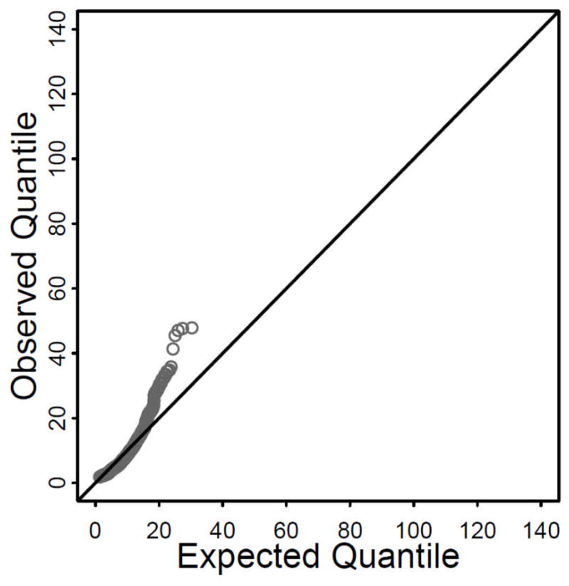
Multivariate QQ Plot of Observed Exogenous Variables (Excluding Product Indictors) of the Illustrative Example

*Note*. Y-axis is the observed quantile (squared Mahalanobis distance).

X-axis is the expected quantile of $χ_{10}^{2}$ distribution.

Following Marsh et al. (2004), each item from the academic self-efficacy scale was matched with an item from the positive family role models scale to form the product terms for the product indicator approaches. Items were matched according to the magnitude of their factor loadings on the underlying construct in a one factor measurement model. Table 10 shows the ML estimates of the interaction model, their ML and SB estimated standard errors, and ML and SB likelihood ratio tests of interaction effect by the four approaches. The estimates of the intercepts and the first order (average) effects (maximum difference = 3.4%), ML SEs (1.2%), and SB SEs (7.4%) differed only slightly. The differences in the estimates and standard errors for the interaction effect γ₃ across estimation approaches was more substantial: Differences in estimates of γ₃ ranged from 2.1% to 18.2%, differences in ML SEs for γ̂₃ ranged from 0% to 44.0%, differences in SB SEs for γ̂₃ ranged from 3.9% to 33.8%. The ML Wald tests of γ₃ varied from z = −2.72 (p = 0.007) for GAPI to z = −1.64 (p = 0.10) for UPI, and the ML LR tests of γ₃ varied from $χ_{1}^{2} = 7.63$ , p = 0.006 for GAPI to $χ_{1}^{2} = 2.69$ , p = 0.10 for UPI. In the present empirical example, of course, we do not know which of these results is correct.

TABLE 10.

Illustrative Example Results Using the Four Approaches

	CPI			GAPI			UPI			LMS
	Est.	SE_ML	SE_SB	Est.	SE_ML	SE_SB	Est.	SE_ML	SE_SB	Est.	SE_ML
Intercept	2.448	0.043 ^**	0.043 ^**	2.448	0.043 ^**	0.043 ^**	2.444	0.043 ^**	0.043 ^**	2.444	0.043 ^**
Positive Family Role Model	0.203	0.053 ^**	0.050 ^**	0.205	0.053 ^**	0.051 ^**	0.203	0.053 ^**	0.051 ^**	0.204	0.053 ^**
Academic Self-Efficacy	0.343	0.085 ^**	0.075 ^**	0.355	0.086 ^**	0.081 ^**	0.349	0.086 ^**	0.079 ^**	0.347	0.086 ^**
Interaction Effect	−0.293	0.109 ^**	0.098 ^**	−0.302	0.111 ^**	0.102 ^**	−0.287	0.175	0.148 ⁺	−0.247	0.098 ^*
LRT of Interaction Effect		7.274 ^**	8.639 ^**		7.634 ^**	8.147 ^**		2.685	2.875		6.556 ^*

Open in a new tab

Note. Est. means parameter estimate. SE_ML means the ML estimated standard error. SE_SB means the Satorra-Bentler correction estimated standard error. LRT means likelihood ratio test.

⁺

p < 0.10,

p < 0.05,

^**

p < 0.01.

Figure 3 probes the interaction effect using simple slope procedures (Aiken & West, 1991; Kelava et al., 2011) based on the results of the conservative UPI approach. The academic performance in 7^th grade was regressed on the academic self-efficacy latent variable in 5^th grade at three levels of positive family role models latent variable in 5^th grade: 1 SD below the mean, at the mean, and 1 SD above the mean. At the mean of positive family role models, effect of academic self-efficacy on academic performance was positive. This positive effect tended to increase as positive family role models decreased, whereas this effect flattened at 1 SD above mean of positive family role models. The children’s self-efficacy latent variable tended to have an increasing effect on the academic performance latent variable as positive family role models latent variable decreased.

Interaction Plot of Positive Family Role Models × Academic Self-Efficacy at 5^th Grade on Academic Performance at 7^th Grade

Discussion

Previous research has been primarily focused on testing latent variable interactions using normal distribution or leptokurtic distributions with modest degrees of skewness and kurtosis of the observed elements in X (< 0.9 and <1.6, respectively). Under these modestly non-normal conditions, the three PI approaches have typically yielded unbiased estimates of the latent interaction effect. The LMS approach yielded unbiased latent interaction effect estimates, but with underestimated SEs when the observed elements in X had |skewness| < 0.5 and kurtosis < 1 (Klein & Moosbrugger, 2000). The modest values of skewness and kurtosis of the observed exogenous variables in previous simulation studies were the result of combining the non-normally distributed exogeneous latent variables ξ₁ and ξ₂ with normally distributed unique factors.

In practice, researchers have no method of estimating the distributions of latent variables and can only use sample values to estimate the population skewness and kurtosis values of the observed variables. Previous research (e.g., Curran et al., 1996; Hu, Bentler, & Kano., 1992) has detected problems (e.g., elevated Type-I error rate) in structural equation modeling without latent variable interactions when data are non-normally distributed. These prior studies have used transformation procedures (e.g., Fleishman, 1978; Vale & Maurelli, 1983) that produce more extreme degrees of non-normality in observed variables than those investigated previously in studies of latent variable interactions.

Wall and Amemiya (2001) pointed out that the latent interaction effect estimate could be biased and inconsistent using the CPI approach when the observed variables in X are nonnormal. In the present simulation study, the symmetric and moderately leptokurtic K1 (kurtosis ≈ 11), the symmetric and highly leptokurtic K2 (kurtosis ≈ 31), and the skewed and moderately leptokurtic $χ_{1}^{2}$ (skewness ≈ 2, kurtosis ≈ 6) distribution conditions generated exogenous observed variables with higher levels of kurtosis than those considered in previous research (Table 2). In these more non-normal conditions, the CPI and LMS approaches overestimated the latent interaction effect and produced inflated Type-I error rates, whereas the UPI and GAPI approaches showed generally unbiased estimates of both the latent interaction and lower-order effects with produced acceptable Type-I error rates once N reached 500.

The present study produced similar findings to those of previous research on the PI approaches with negatively kurtotic distribution conditions (Marsh et al., 2004; Wall & Amemiya, 2001). The results of the uniform condition (skewness = 0; kurtosis ≈ −0.6) generally replicated previous findings using negatively kurtotic distributions: Both the GAPI and UPI approaches yielded unbiased latent interaction and lower-order effects estimates at N ≥ 500. The ML Wald test of CPI and LMS approaches showed acceptable performance in terms of Type-I error rates. The present study is the first to investigate the performance of LMS under negatively kurtotic condition.

In terms of the efficiency of the different approaches, the current results were also consistent with previous findings (e.g., Klein & Moosbrugger, 2000; Marsh et al., 2004). In the normal and uniform conditions, LMS was the most efficient approach, with the lowest mean squared error and smallest SE for the latent interaction effect. The GAPI and UPI approaches were the least efficient in the normal and uniform conditions. Given the substantial bias in the CPI and LMS approaches in the leptokurtic K1, K2, and skewed and leptokurtic $χ_{1}^{2}$ conditions, the GAPI and UPI approaches produced the lowest mean squared error at N ≥ 500.

In the normal and uniform conditions, all approaches with ML yielded acceptable Type-I error rates for the Wald test of latent interaction effect. In the symmetric and leptokurtic K1 and K2 conditions, GAPI and UPI approaches yielded acceptable Type-I error rates for the Wald test at N ≥ 500, except at N = 5000 in the K2 condition. In the skewed and moderately leptokurtic $χ_{1}^{2}$ condition, all approaches typically had slightly inflated Type-I error rates for the Wald test at N ≥ 500. The SB correction was unnecessary in these distribution conditions. Indeed, the results showed that in some conditions, the SB correction yielded inflated Type-I error rates for the Wald and LR test, mitigating against its usage.

The present study was the first to consider the LR test of the latent interaction effect for the PI approaches; this test has previously been considered for the LMS approach (Klein & Moosbrugger, 2000). In linear SEM models, the LR test is asymptotically equivalent to the Wald test. However, the LR test has the advantage of scale independence over the Wald test (Gonzalez & Griffin, 2001), and can produce theoretically more accurate tests of parameters with small sample size (Enders, 2010, pp. 79–80). Similar to the findings for the Wald test, all approaches with ML yielded acceptable Type-I error rates for the LR test of the latent interaction effect at N ≥ 500. Again, the SB correction was unnecessary. Indeed, inflated actual Type-I error rates for the SB LR test occurred in some conditions and estimation failures occurred in others. Comparing the results of the ML LR and Wald tests of the latent interaction effect in terms of statistical power under appropriate conditions (unbiased parameter estimates and acceptable actual Type-I error rates), the LR test had a slight advantage over the Wald test in terms of statistical power.

Contrary to the hope of many SEM researchers (e.g., Marsh et al., 2012), the statistical power of the significance tests of the latent variable interaction under multivariate normality was substantially lower across the four approaches than the theoretical statistical power based on OLS assuming that ξ₁, ξ₂ and η were measured without error. In other words, current SEM approaches to latent variable interaction modeling can correct for bias in the regression coefficients, but may often do so at a substantial cost in statistical power. This finding of a lack of statistical power replicates previous findings by Ma, Aiken, and West (2011) and is consistent with Fuller’s (1987) and Ledgerwood and Shrout’s (2011) observation that latent variable models that correct for measurement error minimize bias, but decrease statistical power. Both the PI and LMS approaches were unable to solve the problem of loss of statistical power due to measurement error (e.g., Aiken & West, 1991).

Conclusions and Limitations

Based on the current findings, we recommend the LMS approach when the observed exogenous variables are symmetric (skewness = 0), and with kurtosis < 1, because it had an advantage in terms of efficiency over the PI approach (see also Kelava et al., 2011). With modestly negatively kurtotic observed variables (kurtosis > −0.75), the LMS approach also outperforms the PI approaches in terms of efficiency, with acceptable bias at larger sample sizes. In distributions with higher levels of positive kurtosis, we recommend the UPI approach which had the best performance at sample sizes ≥ 500. Neither GAPI nor UPI performed well at smaller sample sizes with highly leptokurtic observed variables. Finally, no support for the use of the SB correction was found.

Like other simulation studies, the present study only investigated a limited set of conditions; the results can only be generalized to those conditions. The population effect sizes of the latent interaction effect at the larger sample sizes in the normal condition were small (e.g., N = 1000, f² = .0062; N = 100, f² = .0630 when power = 0.7). The effect size for each sample size was chosen to achieve a theoretical statistical power of 0.7 or 0.9 based on calculations for OLS regression with measurement error free (perfectly reliable) variables. The actual values of statistical power achieved by the SEM approaches were far less than these theoretical values of statistical power. In addition, at the larger sample sizes these values were smaller than the effect sizes that have characterized the empirical literature as summarized by Chaplin (1991), on average 4% of incremental variance accounted for by interaction above and beyond first order effects. Nevertheless, the present findings and conclusions should be generalizable to situations in which the effect sizes of the latent interaction effect are larger. The noncentrality parameter for the latent interaction effect is not available in standard computer software for the PI and LMS approaches, limiting the application of theoretical power analysis procedures (Mooijaart & Satorra, 2009). Mooijaart and Bentler (2010) have proposed an extended ML estimation procedure using third-order moments (i.e., skewness) of some observed variables to estimate the latent interaction effect and noncentrality parameter for power analysis.

A second limitation of current study resulted from a shortcoming of the available procedures for generating non-normal data (Reinartz et al., 2002). The smaller the sample size, the smaller was the univariate kurtosis of the observed variables of X in the K1, K2 and $χ_{1}^{2}$ conditions (Table 4). We investigated several methods of generating non-normal data; all methods shared this limitation. In addition, the population effect sizes of the interaction effect were different in the five sample size conditions. Our study investigated a wide range of different values of kurtosis. However, we did not investigate conditions in which kurtosis was < −0.6 or greater than 31. More negative values of kurtosis appear to be relatively rare in psychological data. Micceri’s (1989) investigation of 440 large scale achievement and psychometric data sets found the most extreme negative value of kurtosis was −1.70 and the most extreme positive value was +37.7.

In summary, our simulation study investigated the performance of four approaches to estimating latent variable interactions over a greater range of distributions of observed exogenous variables than have previously been considered. These conditions included normally distributed, symmetric and negatively kurtotic (kurtosis = −0.60), symmetric and positively kurtotic (kurtosis ≈ 11 and ≈ 31), and moderately skewed and kurtotic (skewness ≈ 2, kurtosis ≈ 6). We recommend the LMS approach when the distribution is approximately normal as it has the greatest statistical power, but maintains acceptable Type-I error and coverage rates. Maximizing statistical power will often be an important consideration since interactions in practice are often small in magnitude and latent variable approaches do not appear to have high statistical power relative to OLS regression of observed scale scores (Ma, 2010; Ma et al., 2011). For distributions with appreciable kurtosis or both skewness and kurtosis, the UPI approach was clearly preferable at larger sample sizes (N ≥ 500). Neither the use of the ML LR test nor the SB correction of the standard errors appreciably improved the performance of any of the approaches.

Supplementary Material

table 1

NIHMS405516-supplement-table_1.pdf^{(15.8KB, pdf)}

table 2

NIHMS405516-supplement-table_2.pdf^{(60KB, pdf)}

table 3

NIHMS405516-supplement-table_3.pdf^{(71.6KB, pdf)}

table 4

NIHMS405516-supplement-table_4.pdf^{(49.8KB, pdf)}

Acknowledgments

We thank Mark Roosa, Jenn-Yun Tein, and Proyeto: La Familia (The Family Project); NIMH Grant R01 MH68920, culture, context, and Mexican American mental health, at the Prevention Research Center, Arizona State University who generously provided data for the example. Stephen G. West was partially supported by a Forschungspreis (research prize) from the Alexander von Humboldt Foundation.

Footnotes

Throughout this manuscript, kurtosis is defined as excess kurtosis having a value of 0 for a normally distributed variable.

References

Aiken LS, West SG. Multiple regression: Testing and interpreting interactions. Newbury, CA: Sage; 1991. [Google Scholar]
Bollen KA. Structural equations with latent variables. New York: Wiley; 1989. [Google Scholar]
Chou CP, Bentler PM, Satorra A. Scaled test statistics and robust standard errors for non-normal data in covariance structure analysis: A Monte Carlo study. British Journal of Mathematical and Statistical Psychology. 1991;44(2):347–357. doi: 10.1111/j.2044-8317.1991.tb00966.x. [DOI] [PubMed] [Google Scholar]
Coenders G, Batista-Foguet JM, Saris WE. Simple, efficient and distribution-free approach to interaction effects in complex structural equation models. Quality and Quantity. 2008;42(3):369–396. [Google Scholar]
Collins LM, Schafer JL, Kam CM. A comparison of inclusive and restrictive strategies in modern missing data procedures. Psychological Methods. 2001;6(4):330–351. [PubMed] [Google Scholar]
Chaplin WF. The next generation of moderator research in personality psychology. Journal of Personality. 1991;59(2):143–178. doi: 10.1111/j.1467-6494.1991.tb00772.x. [DOI] [PubMed] [Google Scholar]
Curran PJ, West SG, Finch JF. The robustness of test statistics to nonnormality and specification error in confirmatory factor analysis. Psychological Methods. 1996;1(1):16–29. [Google Scholar]
Enders CK. Applied missing data analysis. New York: Guilford; 2010. [Google Scholar]
Fleishman AI. A method for simulating non-normal distributions. Psychometrika. 1978;43(4):521–532. [Google Scholar]
Flora DB, Curran PJ. An empirical evaluation of alternative methods of estimation for confirmatory factor analysis with ordinal data. Psychological Methods. 2004;9(4):466–491. doi: 10.1037/1082-989X.9.4.466. [DOI] [PMC free article] [PubMed] [Google Scholar]
Friendly M. Statistical graphics for multivariate data. Proceedings of the SAS SUGI 16 Conference; 1991. Retrieved from http://www.math.yorku.ca/SCS/sugi/sugi16-paper.html. [Google Scholar]
Fuller WA. Measurement error models. New York: Wiley; 1987. [Google Scholar]
Gonzalez R, Griffin D. Testing parameters in structural equation modeling: Every “one” matters. Psychological Methods. 2001;6(3):258–269. doi: 10.1037/1082-989x.6.3.258. [DOI] [PubMed] [Google Scholar]
Hu LT, Bentler PM. Fit indices in covariance structure modeling: Sensitivity to underparameterized model misspecification. Psychological Methods. 1998;3(4):424–453. [Google Scholar]
Hu L, Bentler PM, Kano Y. Can test statistics in covariance structure analysis be trusted? Psychological Bulletin. 1992;112(2):351–362. doi: 10.1037/0033-2909.112.2.351. [DOI] [PubMed] [Google Scholar]
Jaccard J, Wan CK. Measurement error in the analysis of interaction effects between continuous predictors using multiple regression: Multiple indicator and structural equation approaches. Psychological Bulletin. 1995;117(2):348–357. [Google Scholar]
Jöreskog KG, Yang F. Nonlinear structural equation models: The Kenny-Judd model with interaction effects. In: Schumacker E, Marcoulides GA, editors. Advanced structural equation modeling: Issues and techniques. Mahwah, NJ: Erlbaum; 1996. pp. 57–88. [Google Scholar]
Kelava A, Werner C, Schermelleh-Engel K, Moosbrugger H, Zapf D, Ma Y, Cham H, Aiken LS, West SG. Advanced nonlinear structural equation modeling: Theoretical properties and empirical application of the LMS and QML estimators. Structural Equation Modeling. 2011;18(3):465–491. [Google Scholar]
Kenny DA, Judd CM. Estimating the nonlinear and interactive effects of latent variables. Psychological Bulletin. 1984;96(1):201–210. [Google Scholar]
Klein AG, Moosbrugger H. Maximum likelihood estimation of latent interaction effects with the LMS method. Psychometrika. 2000;65(4):457–474. [Google Scholar]
Klein AG, Muthén BO. Quasi-maximum likelihood estimation of structural equation models with multiple interaction and quadratic effects. Multivariate Behavioral Research. 2007;42(4):647–673. [Google Scholar]
Klein AG, Schermelleh-Engel K, Moosbrugger H, Kelava A. Assessing spurious interaction effects. In: Teo T, Khine MS, editors. Structural equation modeling in educational research: Concepts and applications. Rotterdam, The Netherlands: Sense Publishers; 2009. pp. 13–28. [Google Scholar]
Ledgerwood A, Shrout PE. The trade-off between accuracy and precision in latent variable models of mediation processes. Journal of Personality and Social Psychology. 2011;101(6):1174–1188. doi: 10.1037/a0024776. [DOI] [PMC free article] [PubMed] [Google Scholar]
Ma Y. Unpublished doctoral dissertation. Arizona State University; 2010. Comparison of statistical power for testing interactive versus quadratic effects. [Google Scholar]
Ma Y, Aiken LS, West SG. Comparison of statistical power for testing interactive versus quadratic effects using measured variable versus latent variable approaches. Paper presented at the meeting of the American Statistical Association; Miami, FL. 2011. Aug, [Google Scholar]
Marsh HW, Wen Z, Hau KT. Structural equation models of latent interactions: Evaluation of alternative estimation strategies and indicator construction. Psychological Methods. 2004;9(3):275–300. doi: 10.1037/1082-989X.9.3.275. [DOI] [PubMed] [Google Scholar]
Marsh HW, Wen Z, Nagengast B, Hau KT. Structural equation models of latent interaction. In: Hoyle RH, editor. Handbook of structural equation modeling. New York: Guilford; 2012. pp. 436–458. [Google Scholar]
Mattson S. How to generate nonnormal data for simulation of structural equation models. Multivariate Behavioral Research. 1997;32(4):355–373. doi: 10.1207/s15327906mbr3204_3. [DOI] [PubMed] [Google Scholar]
Micceri T. The unicorn, the normal curve, and other improbable creatures. Psychological Bulletin. 1989;105(1):156–166. [Google Scholar]
Midgley C, Maehr ML, Hruda LZ, Anderman E, Anderman L, Freeman KE, Gheen M, Kaplan A, Kumar R, Middleton MJ, Nelson J, Roeser R, Urdan T. Manual for the patterns of adaptive learning scale. Ann Arbor: University of Michigan; 2000. [Google Scholar]
Mooijaart A, Bentler PM. An alternative approach for nonlinear latent variable models. Structural Equation Modeling. 2010;17(3):357–373. [Google Scholar]
Mooijaart A, Satorra A. On insensitivity of the chi-square model test to nonlinear misspecification in structural equation models. Psychometrika. 2009;74(3):443–455. [Google Scholar]
Muthén LK, Muthén BO. Mplus User’s Guide. 6. Los Angeles, CA: Muthén & Muthén; 1998–2010. [Google Scholar]
Reinartz WJ, Echambadi R, Chin WW. Generating non-normal data for simulation of structural equation models using Mattson’s method. Multivariate Behavioral Research. 2002;37(2):227–244. [Google Scholar]
Roosa MW, Liu FF, Torres M, Gonzales NA, Knight GP, Saenz D. Sampling and recruitment in studies of cultural influences on adjustment: a case study with Mexican Americans. Journal of Family Psychology. 2008;22(2):293–302. doi: 10.1037/0893-3200.22.2.293. [DOI] [PMC free article] [PubMed] [Google Scholar]
Roosa MW, O’Donnell M, Cham H, Gonzales NA, Zeiders KH, Tein JY, Knight GP, Umaña-Taylor A. A prospective study of Mexican American adolescents’ academic success: Considering family and individual factors. Journal of Youth and Adolescence. 2012;41(3):307–319. doi: 10.1007/s10964-011-9707-x. [DOI] [PMC free article] [PubMed] [Google Scholar]
Satorra A, Bentler PM. A scaled difference chi-square test statistic for moment structure analysis. Psychometrika. 2001;66(4):507–514. doi: 10.1007/s11336-009-9135-y. [DOI] [PMC free article] [PubMed] [Google Scholar]
Satorra A, Bentler PM. Ensuring positiveness of the scaled difference chi-square test statistic. Psychometrika. 2010;75(2):243–248. doi: 10.1007/s11336-009-9135-y. [DOI] [PMC free article] [PubMed] [Google Scholar]
Savalei V. Small sample statistics for incomplete nonnormal data: extensions of complete data formulae and a Monte Carlo comparison. Structural Equation Modeling. 2010;17(2):241–264. [Google Scholar]
Schermelleh-Engel K, Klein AG, Moosbrugger H. Estimating nonlinear effects using a latent moderated structural equations approach. In: Schumacker E, Marcoulides GA, editors. Interaction and nonlinear effects in structural equation modeling. Mahwah, NJ: Erlbaum; 1998. pp. 203–238. [Google Scholar]
Vale CD, Maurelli VA. Simulating multivariate nonnormal distributions. Psychometrika. 1983;48(3):465–471. [Google Scholar]
Wall MM, Amemiya Y. Generalized appended product indicator procedure for nonlinear structural equation analysis. Journal of Educational and Behavioral Statistics. 2001;26(1):1–29. [Google Scholar]
Wall MM, Amemiya Y. A method of moments technique for fitting interaction effects in structural equation models. British Journal of Mathematical and Statistical Psychology. 2003;56(1):47–63. doi: 10.1348/000711003321645331. [DOI] [PubMed] [Google Scholar]
West SG, Finch JF, Curran PJ. Structural equation models with nonnormal variables: Problems and remedies. In: Hoyle RH, editor. Structural equation modeling: Concepts, issues, and applications. Thousand Oaks, CA: Sage; 1995. pp. 56–75. [Google Scholar]
Yuan KH, Bentler PM, Zhang W. The effect of skewness and kurtosis on mean and covariance structure analysis. Sociological Methods & Research. 2005;34(2):240–258. [Google Scholar]

Associated Data

This section collects any data citations, data availability statements, or supplementary materials included in this article.

Supplementary Materials

table 1

NIHMS405516-supplement-table_1.pdf^{(15.8KB, pdf)}

table 2

NIHMS405516-supplement-table_2.pdf^{(60KB, pdf)}

table 3

NIHMS405516-supplement-table_3.pdf^{(71.6KB, pdf)}

table 4

NIHMS405516-supplement-table_4.pdf^{(49.8KB, pdf)}

[R1] Aiken LS, West SG. Multiple regression: Testing and interpreting interactions. Newbury, CA: Sage; 1991. [Google Scholar]

[R2] Bollen KA. Structural equations with latent variables. New York: Wiley; 1989. [Google Scholar]

[R3] Chou CP, Bentler PM, Satorra A. Scaled test statistics and robust standard errors for non-normal data in covariance structure analysis: A Monte Carlo study. British Journal of Mathematical and Statistical Psychology. 1991;44(2):347–357. doi: 10.1111/j.2044-8317.1991.tb00966.x. [DOI] [PubMed] [Google Scholar]

[R4] Coenders G, Batista-Foguet JM, Saris WE. Simple, efficient and distribution-free approach to interaction effects in complex structural equation models. Quality and Quantity. 2008;42(3):369–396. [Google Scholar]

[R5] Collins LM, Schafer JL, Kam CM. A comparison of inclusive and restrictive strategies in modern missing data procedures. Psychological Methods. 2001;6(4):330–351. [PubMed] [Google Scholar]

[R6] Chaplin WF. The next generation of moderator research in personality psychology. Journal of Personality. 1991;59(2):143–178. doi: 10.1111/j.1467-6494.1991.tb00772.x. [DOI] [PubMed] [Google Scholar]

[R7] Curran PJ, West SG, Finch JF. The robustness of test statistics to nonnormality and specification error in confirmatory factor analysis. Psychological Methods. 1996;1(1):16–29. [Google Scholar]

[R8] Enders CK. Applied missing data analysis. New York: Guilford; 2010. [Google Scholar]

[R9] Fleishman AI. A method for simulating non-normal distributions. Psychometrika. 1978;43(4):521–532. [Google Scholar]

[R10] Flora DB, Curran PJ. An empirical evaluation of alternative methods of estimation for confirmatory factor analysis with ordinal data. Psychological Methods. 2004;9(4):466–491. doi: 10.1037/1082-989X.9.4.466. [DOI] [PMC free article] [PubMed] [Google Scholar]

[R11] Friendly M. Statistical graphics for multivariate data. Proceedings of the SAS SUGI 16 Conference; 1991. Retrieved from http://www.math.yorku.ca/SCS/sugi/sugi16-paper.html. [Google Scholar]

[R12] Fuller WA. Measurement error models. New York: Wiley; 1987. [Google Scholar]

[R13] Gonzalez R, Griffin D. Testing parameters in structural equation modeling: Every “one” matters. Psychological Methods. 2001;6(3):258–269. doi: 10.1037/1082-989x.6.3.258. [DOI] [PubMed] [Google Scholar]

[R14] Hu LT, Bentler PM. Fit indices in covariance structure modeling: Sensitivity to underparameterized model misspecification. Psychological Methods. 1998;3(4):424–453. [Google Scholar]

[R15] Hu L, Bentler PM, Kano Y. Can test statistics in covariance structure analysis be trusted? Psychological Bulletin. 1992;112(2):351–362. doi: 10.1037/0033-2909.112.2.351. [DOI] [PubMed] [Google Scholar]

[R16] Jaccard J, Wan CK. Measurement error in the analysis of interaction effects between continuous predictors using multiple regression: Multiple indicator and structural equation approaches. Psychological Bulletin. 1995;117(2):348–357. [Google Scholar]

[R17] Jöreskog KG, Yang F. Nonlinear structural equation models: The Kenny-Judd model with interaction effects. In: Schumacker E, Marcoulides GA, editors. Advanced structural equation modeling: Issues and techniques. Mahwah, NJ: Erlbaum; 1996. pp. 57–88. [Google Scholar]

[R18] Kelava A, Werner C, Schermelleh-Engel K, Moosbrugger H, Zapf D, Ma Y, Cham H, Aiken LS, West SG. Advanced nonlinear structural equation modeling: Theoretical properties and empirical application of the LMS and QML estimators. Structural Equation Modeling. 2011;18(3):465–491. [Google Scholar]

[R19] Kenny DA, Judd CM. Estimating the nonlinear and interactive effects of latent variables. Psychological Bulletin. 1984;96(1):201–210. [Google Scholar]

[R20] Klein AG, Moosbrugger H. Maximum likelihood estimation of latent interaction effects with the LMS method. Psychometrika. 2000;65(4):457–474. [Google Scholar]

[R21] Klein AG, Muthén BO. Quasi-maximum likelihood estimation of structural equation models with multiple interaction and quadratic effects. Multivariate Behavioral Research. 2007;42(4):647–673. [Google Scholar]

[R22] Klein AG, Schermelleh-Engel K, Moosbrugger H, Kelava A. Assessing spurious interaction effects. In: Teo T, Khine MS, editors. Structural equation modeling in educational research: Concepts and applications. Rotterdam, The Netherlands: Sense Publishers; 2009. pp. 13–28. [Google Scholar]

[R23] Ledgerwood A, Shrout PE. The trade-off between accuracy and precision in latent variable models of mediation processes. Journal of Personality and Social Psychology. 2011;101(6):1174–1188. doi: 10.1037/a0024776. [DOI] [PMC free article] [PubMed] [Google Scholar]

[R24] Ma Y. Unpublished doctoral dissertation. Arizona State University; 2010. Comparison of statistical power for testing interactive versus quadratic effects. [Google Scholar]

[R25] Ma Y, Aiken LS, West SG. Comparison of statistical power for testing interactive versus quadratic effects using measured variable versus latent variable approaches. Paper presented at the meeting of the American Statistical Association; Miami, FL. 2011. Aug, [Google Scholar]

[R26] Marsh HW, Wen Z, Hau KT. Structural equation models of latent interactions: Evaluation of alternative estimation strategies and indicator construction. Psychological Methods. 2004;9(3):275–300. doi: 10.1037/1082-989X.9.3.275. [DOI] [PubMed] [Google Scholar]

[R27] Marsh HW, Wen Z, Nagengast B, Hau KT. Structural equation models of latent interaction. In: Hoyle RH, editor. Handbook of structural equation modeling. New York: Guilford; 2012. pp. 436–458. [Google Scholar]

[R28] Mattson S. How to generate nonnormal data for simulation of structural equation models. Multivariate Behavioral Research. 1997;32(4):355–373. doi: 10.1207/s15327906mbr3204_3. [DOI] [PubMed] [Google Scholar]

[R29] Micceri T. The unicorn, the normal curve, and other improbable creatures. Psychological Bulletin. 1989;105(1):156–166. [Google Scholar]

[R30] Midgley C, Maehr ML, Hruda LZ, Anderman E, Anderman L, Freeman KE, Gheen M, Kaplan A, Kumar R, Middleton MJ, Nelson J, Roeser R, Urdan T. Manual for the patterns of adaptive learning scale. Ann Arbor: University of Michigan; 2000. [Google Scholar]

[R31] Mooijaart A, Bentler PM. An alternative approach for nonlinear latent variable models. Structural Equation Modeling. 2010;17(3):357–373. [Google Scholar]

[R32] Mooijaart A, Satorra A. On insensitivity of the chi-square model test to nonlinear misspecification in structural equation models. Psychometrika. 2009;74(3):443–455. [Google Scholar]

[R33] Muthén LK, Muthén BO. Mplus User’s Guide. 6. Los Angeles, CA: Muthén & Muthén; 1998–2010. [Google Scholar]

[R34] Reinartz WJ, Echambadi R, Chin WW. Generating non-normal data for simulation of structural equation models using Mattson’s method. Multivariate Behavioral Research. 2002;37(2):227–244. [Google Scholar]

[R35] Roosa MW, Liu FF, Torres M, Gonzales NA, Knight GP, Saenz D. Sampling and recruitment in studies of cultural influences on adjustment: a case study with Mexican Americans. Journal of Family Psychology. 2008;22(2):293–302. doi: 10.1037/0893-3200.22.2.293. [DOI] [PMC free article] [PubMed] [Google Scholar]

[R36] Roosa MW, O’Donnell M, Cham H, Gonzales NA, Zeiders KH, Tein JY, Knight GP, Umaña-Taylor A. A prospective study of Mexican American adolescents’ academic success: Considering family and individual factors. Journal of Youth and Adolescence. 2012;41(3):307–319. doi: 10.1007/s10964-011-9707-x. [DOI] [PMC free article] [PubMed] [Google Scholar]

[R37] Satorra A, Bentler PM. A scaled difference chi-square test statistic for moment structure analysis. Psychometrika. 2001;66(4):507–514. doi: 10.1007/s11336-009-9135-y. [DOI] [PMC free article] [PubMed] [Google Scholar]

[R38] Satorra A, Bentler PM. Ensuring positiveness of the scaled difference chi-square test statistic. Psychometrika. 2010;75(2):243–248. doi: 10.1007/s11336-009-9135-y. [DOI] [PMC free article] [PubMed] [Google Scholar]

[R39] Savalei V. Small sample statistics for incomplete nonnormal data: extensions of complete data formulae and a Monte Carlo comparison. Structural Equation Modeling. 2010;17(2):241–264. [Google Scholar]

[R40] Schermelleh-Engel K, Klein AG, Moosbrugger H. Estimating nonlinear effects using a latent moderated structural equations approach. In: Schumacker E, Marcoulides GA, editors. Interaction and nonlinear effects in structural equation modeling. Mahwah, NJ: Erlbaum; 1998. pp. 203–238. [Google Scholar]

[R41] Vale CD, Maurelli VA. Simulating multivariate nonnormal distributions. Psychometrika. 1983;48(3):465–471. [Google Scholar]

[R42] Wall MM, Amemiya Y. Generalized appended product indicator procedure for nonlinear structural equation analysis. Journal of Educational and Behavioral Statistics. 2001;26(1):1–29. [Google Scholar]

[R43] Wall MM, Amemiya Y. A method of moments technique for fitting interaction effects in structural equation models. British Journal of Mathematical and Statistical Psychology. 2003;56(1):47–63. doi: 10.1348/000711003321645331. [DOI] [PubMed] [Google Scholar]

[R44] West SG, Finch JF, Curran PJ. Structural equation models with nonnormal variables: Problems and remedies. In: Hoyle RH, editor. Structural equation modeling: Concepts, issues, and applications. Thousand Oaks, CA: Sage; 1995. pp. 56–75. [Google Scholar]

[R45] Yuan KH, Bentler PM, Zhang W. The effect of skewness and kurtosis on mean and covariance structure analysis. Sociological Methods & Research. 2005;34(2):240–258. [Google Scholar]

PERMALINK

Estimating Latent Variable Interactions With Non-Normal Observed Data: A Comparison of Four Approaches

Heining Cham

Stephen G West

Yue Ma

Leona S Aiken

Abstract

Product Indicator Approach

TABLE 1.

Latent Moderated Structural Equations Approach

The Satorra-Bentler Correction

Significance Testing of the Interaction Effect for the PI and LMS Approaches

Overview of Previous Literature

TABLE 2.

Univariate Skewness and Kurtosis

PI Approach

LMS Approach

Research Questions

Method

(1) Sample size N: 100, 200, 500, 1000, 5000

(2) Interaction Model

TABLE 3.

(3) Distributions of ξ1, ξ2, and δ

TABLE 4.

Figure 1.

(4) Latent variable interaction estimators

Results

Model Convergence Rates

Relative Bias of Latent Interaction Effect Estimate

TABLE 5.

Mean Square Error, Standard Error Ratio, and Coverage Rate of Estimates of the Latent Interaction Effect

TABLE 6.

TABLE 7.

Performance of Lower Order Effects

Type-I Error Rate and Statistical Power

TABLE 8.

TABLE 9.

Actual Type-I Error Rate of Latent Interaction Effect

Actual Statistical Power of Latent Interaction Effect

Illustrative Example

Description

Analysis

Figure 2.

TABLE 10.

Figure 3.

Discussion

Conclusions and Limitations

Supplementary Material

Acknowledgments

Footnotes

References

Associated Data

Supplementary Materials

ACTIONS

PERMALINK

RESOURCES

Similar articles

Cited by other articles

Links to NCBI Databases

(3) Distributions of ξ₁, ξ₂, and δ