Physiological noise reduction using volumetric functional magnetic resonance inverse imaging

Abstract

Physiological noise arising from a variety of sources can significantly degrade the detection of task‐related activity in BOLD‐contrast fMRI experiments. If whole head spatial coverage is desired, effective suppression of oscillatory physiological noise from cardiac and respiratory fluctuations is quite difficult without external monitoring, since traditional EPI acquisition methods cannot sample the signal rapidly enough to satisfy the Nyquist sampling theorem, leading to temporal aliasing of noise. Using a combination of high speed magnetic resonance inverse imaging (InI) and digital filtering, we demonstrate that it is possible to suppress cardiac and respiratory noise without auxiliary monitoring, while achieving whole head spatial coverage and reasonable spatial resolution. Our systematic study of the effects of different moving average (MA) digital filters demonstrates that a MA filter with a 2 s window can effectively reduce the variance in the hemodynamic baseline signal, thereby achieving 57%–58% improvements in peak z‐statistic values compared to unfiltered InI or spatially smoothed EPI data (FWHM = 8.6 mm). In conclusion, the high temporal sampling rates achievable with InI permit significant reductions in physiological noise using standard temporal filtering techniques that result in significant improvements in hemodynamic response estimation. Hum Brain Mapp, 2012. © 2011 Wiley Periodicals, Inc.

INTRODUCTION

Functional MRI (fMRI) allows noninvasive detection of neural activity changes coupled with blood‐oxygen level dependent (BOLD) contrast mechanisms that are based on deoxyhemoglobin serving as an endogenous contrast agent [Kwong et al., 1992; Ogawa et al., 1990]. In BOLD‐contrast fMRI, neuronal activity is associated with a complex series of hemodynamic changes, including blood flow, volume, and oxygenation modulations, whose net effect results in MRI signal increase or decrease [Logothetis et al., 2001]. In most measurement environments, the hemodynamic signal changes related to task induced neural activity are quite small. Many factors can contribute to the total signal variation in addition to the experimental effects of interest, which complicates the task of isolating the components reflecting changes in neural activity.

The noise sources confounding the BOLD‐contrast fMRI data processing can be categorized into two types: system noise and sample noise. System noise can arise from suboptimal instrument performance. This includes, but is not limited to, thermal noise in the radio‐frequency coils, preamplifiers, and other electronic components in the receiver processing chain. Sample noise is related to the properties of the object to be imaged. For example, resistive and dielectric losses due to the presence of the sample inside the RF coil contribute to sample noise. In fMRI experiments, motion during data acquisition is another significant source of noise [Hajnal et al., 1994]. Motion effects can be effectively reduced by either restricting movement of the participant's head inside the RF coil or using image volume alignment to reduce image‐to‐image signal variation under the assumption of rigid body motion between acquisitions [Cox and Jesmanowicz, 1999; Woods et al., 1998]. Other sources of sample noise can result from intrinsic physiological processes. In fMRI experiments, physiological noise can be further separated into echo‐time and non‐echo‐time dependent components [Kruger and Glover, 2001], with the latter component closely related to periodic cardiac and respiratory activity. Comparing system and sample noise in terms of improving contrast‐to‐noise ratio (CNR) in high field fMRI experiments, the latter constitutes the major limitation. Physiological noise is generally proportional to the signal and going to higher field strength increases its contribution to overall variance [Kruger and Glover, 2001]. In addition, at a given field (e.g. 3 T), improvements to receiver hardware and signal reception [Bodurka et al., 2007] can result in phyisological noise dominating the variance in fMRI time‐course data.

Cardiac pulsations cause cerebrospinal fluid (CSF) and brain parenchyma movement resulting from cyclic vascular pressure changes interacting with the incompressible property of both tissues. Periodically increased intracranial pressure leads to repetitive downward parenchymal shifts because of the anisotropic distribution of pressure resistance [Feinberg, 1992; Feinberg and Mark, 1987; Poncelet et al., 1992]. Parenchymal motion related to cardiac pulsation causes oscillatory image intensity changes in BOLD‐contrast fMRI time series [Shmueli et al., 2007]. It has been shown that the resulting signal artifacts are particularly prominent near the vertebrobasilar vascular system near the center of the brain, and around the anterior cerebral artery in the anterior interhemispheric fissure between the medial frontal lobes [Dagli et al., 1999]. In a similar fashion, respiration can cause bulk susceptibility modulations from organ movement outside the imaging FOV, leading to both oscillatory magnetic field changes inside the FOV and consequent signal changes in BOLD‐contrast fMRI time series [Windischberger et al., 2002]. These artifacts are usually found in CSF and surrounding tissues [Birn et al., 2006]. Cardiac and respiratory related noise account for approximately 33% of the total physiological noise encountered in human gray matter in fMRI studies performed at 3T [Birn et al., 2006; Kruger and Glover, 2001]. In addition, physiological noise sources are the dominant limiting factor in high‐field fMRI [Kruger and Glover, 2001]. It should be noted that other low‐frequency physiological noise sources are not solely due to the aliasing of periodic cardiac pulsations and respiration. The low‐frequency (<0.1 Hz) physiological noise arising primarily from CO₂ effects resulting from variations in ventilatory volume [Birn et al., 2006; Shmueli et al., 2007; Wise et al., 2004] may be more related to the BOLD‐like physiological noise component in Kruger and Glover's classification [Kruger and Glover, 2001]. Regardless of the source of fluctuation in fMRI time series, more effective methods to remove these unwanted signal components could improve the sensitivity and specificity of task‐related signal detection.

A number of methods to reduce the physiological noise in BOLD‐contrast fMRI have been explored. Early work used narrow‐band notch filtering to reduce the effects of cardiac and respiratory fluctuations based on the assumed periodicity of these signals [Biswal et al., 1996]. In these experiments, pulse oximeter recordings were used to estimate the frequency contributions of cardiac and respiratory activity in the BOLD‐contrast time series. Next, using this frequency information, finite impulse response band‐reject digital filters were constructed to remove the effects of physiological fluctuations. Although effective, widespread adoption of this band‐reject filtering technique has been limited, possibly due to the availability of alternative methods. In other studies, retrospective gating in k‐space [Hu et al., 1995] and image space [Glover et al., 2000] were used to suppress physiological noise using data‐driven adaptive algorithms. The RETROKCOR method can suppress fluctuations in cardiac and respiratory frequency ranges by 5% and 20% respectively; and the RETROICOR method can suppress fluctuations in the cardiac and respiratory frequency ranges by 68% and 50% respectively [Glover et al., 2000]. Use of adaptive filters has been suggested as a means to suppress cardiac and respiratory noise: the hemodynamic baseline fluctuation can be suppressed by 10% on average and 50% maximally, comparable to RETROICOR method [Deckers et al., 2006]. More sophisticated multivariate methods using Independent Component Analysis (ICA) and Principle Component Analysis (PCA) can remove periodic physiological noise after spatiotemporal data decomposition and identification of cardiac and respiratory components [Thomas et al., 2002]. In addition, navigator echoes have been used to map respiratory related brain motion and therefore to reduce physiological noise in fMRI time series [Barry and Menon, 2005; Hu and Kim, 1994; Pfeuffer et al., 2002]. However, relatively little spatial information can be acquired using navigator echoes, limiting their ability to spatially resolve physiological noise sources.

In all attempts to mitigate the effects of physiological noise in fMRI experiments, there are two competing factors: the image volume sampling rate and spatial coverage. Currently, echo‐planar imaging (EPI) requires approximately 2 ‐ 4 s to acquire a full brain volume. At this sampling rate, EPI has a TR sufficiently short to ensure that low‐frequency (<0.1 Hz) noise sources can be adequately sampled. However, EPI lacks sufficient temporal resolution to avoid aliasing of higher frequency periodic cardiac and respiratory effects. In general, time series acquired at low sampling frequencies are difficult to digitally denoise because the frequency components of the aliased noise are distributed in other parts of the frequency spectrum. If the sampling frequency is below the Nyquist sampling frequency, external monitoring devices, such as pulse oximeters or respirometer belts can help identify aliased cardiac and respiratory signals and thereby suggest the optimal filter needed for their removal. An alternative strategy would be to increase the acquisition sampling rate in order to satisfy the Nyquist sampling theorem, thereby allowing straightforward removal of periodic, pulsatile cardiac and respiratory temporal noise. However, implementing this solution using standard EPI techniques severely limits spatial coverage. For example, if a single‐shot single slice EPI takes 60 ms to acquire, a volumetric acquisition of 8 slices has an effective volumetric sampling rate of 480 ms, which is sufficient to resolve cardiac cycles with a period of 1 s. Using a customary 5 mm slice thickness, spatial extent is then limited to a 40 mm thick slab, far short of the approximately 150 mm slab needed for whole‐brain coverage. It follows that an imaging technique allowing acquisition of whole brain volumes at sampling rates sufficient to fully capture cardiac and respiratory effects might allow more effective mitigation of physiological noise.

Here we study the use of magnetic resonance inverse imaging (InI) [Lin et al., 2006, 2008a, b] in suppressing physiological noise using relatively simple digital filters. No external physiological monitoring devices were needed and the spatial coverage allowed whole brain imaging with spatial resolution comparable with conventional fMRI acquisition protocols. The development of InI was inspired by the physical similarity between the geometry of dense coil arrays in MRI and the sensor arrays used in modern magnetoencephalography (MEG) and electroencephalography (EEG) systems. Mathematically, InI image reconstruction is an extreme form of parallel MRI, an approach that can accelerate image acquisition using disparate spatial information sampled from the channels of a receiver coil array [Pruessmann et al., 1999; Sodickson and Manning, 1997]. Using multiple radiofrequency array elements to cover the brain, InI can achieve fast spatial encoding by minimizing k‐space traversal and then solving the inverse problem using data simultaneously acquired from all coil elements. This approach is closely related to other massively parallel MRI techniques, including the single‐echo‐acquisition (SEA) method [McDougall and Wright, 2005] and the one‐voxel‐one‐coil (OVOC) MR‐encephalography technique [Hennig et al., 2007]. Minimal gradient data encoding has also been utilized in back projection reconstruction (HPYR) of MR angiography [Mistretta et al., 2006]. Our previous efforts have focused on formulating the relationship between the spatial information contained in the different channels of the RF coil array with full or minimal gradient encoding [Lin et al., 2006, 2008a].

In this article we demonstrate advantages in using a temporal filter to process BOLD‐contrast fMRI signals obtained using InI's high temporal resolution. This approach allows direct suppression of the periodic cardiac and respiratory disturbances contained in functional time series without the need for external monitoring devices. Since InI can achieve 100 ms temporal resolution and whole‐brain spatial coverage with reasonable spatial resolution, it is possible to optimize digital moving average (MA) low‐pass filters in order to effectively suppress physiological noise. For this feasibility study, we chose a simple MA low‐pass filter because of its robustness and ease of implementation. Intuitively, a MA filter with an overly short temporal window cannot suppress oscillatory cardiac and respiratory noise effectively, while a MA filter with an overly long window suppresses not only noise but also the image contrast between the baseline and the task conditions. Therefore, an optimal filter length should exist for physiological noise suppression in functional imaging studies.

We utilized data from a previous visual experiment, which was acquired using InI techniques [Lin et al., 2008a]. The motivation for utilizing an existing data set is to facilitate comparisons with the previous InI data modeling approaches. First, we systematically varied the noise‐suppressing filter parameters to compare their respective effects on detection sensitivity. Then we describe methods for quantifying detection power in the filtered and unfiltered InI data. Finally, we demonstrate how the use of an optimized MA filter can improve the sensitivity of detecting task‐related regional BOLD‐contrast responses in high temporal resolution (100 ms) InI time series.

METHODS

Participants

Six healthy participants were recruited for the study. Informed consent was obtained from each participant under conditions approved by the Institutional Review Board of Massachusetts General Hospital.

Task

Participants were asked to maintain fixation at the center of a tangent screen during periodic presentation of a high‐contrast visual checkerboard reversing at 8 Hz. The checkerboard stimulus subtended 20° of visual angle and was generated from 24 evenly distributed radial wedges (15° each) and 8 concentric rings of equal width. The stimuli were generated using Psychtoolbox [Brainard, 1997; Pelli, 1997] running under Matlab (The Mathworks, Natick, MA). The reversing checkerboard stimuli were presented for 500 ms and the onset of each presentation was randomized such that the inter‐stimulus intervals varied uniformly between 3 and 16 s. Thirty‐two stimulation trials were presented during each of four 240 s runs, resulting in a total of 128 trials per participant. Additionally, we collected one “resting state” run, where the participant was asked to remain still, keep his eyes open, and stay alert in the magnet, during which time no stimulus was presented. The same data set has been used in our previously published work on InI technical development [Lin et al., 2008a].

Image Data Acquisition

MRI data were collected with a 3T MRI scanner (Tim Trio, Siemens Medical Solutions, Erlangen, Germany), using a body transmit coil and a 32‐channel head array receive coil. Using volumetric InI, each image volume time point was collected by a 3D multishot EPI pulse sequence with frequency and phase encodings. The partition encoding was only implemented in the reference scan and the accelerated acquisition was obtained by leaving out the partition encoding. Volumetric image reconstruction was achieved by solving inverse problems in the partition encoding direction.

The InI reference scan was collected using a 3D multishot EPI readout, exciting one thick slab covering the entire brain (FOV 256 mm × 256 mm × 256 mm; 64 × 64 × 64 image matrix), and setting the flip angle to the Ernst angle of 30⁰. Partition encoding was used to obtain the spatial information along the left‐right axis. InI uses EPI frequency and phase encoding along the inferior‐superior and anterior‐posterior axes respectively. We used TR = 100 ms, TE = 30 ms, bandwidth = 2,604 Hz and a 12.8 s total acquisition time for the reference scan, which included 64 TRs allowing coverage of a volume comprising 64 partitions with two repetitions.

The InI functional scans used the same volume prescription, TR, TE, flip angle, and bandwidth as the ones used for the InI reference scan. The principal difference was that the partition encoding was omitted: the full volume was excited, and the spins were spatially encoded only by a single‐slice EPI trajectory, resulting in a sagittal Y‐Z projection image with spatially collapsed data along the left‐right (X) direction. The InI reconstruction algorithm, described in the next section, was then used to estimate the spatial information along the X axis. In each run, we collected 2,400 measurements after 32 dummy measurements in order to reach longitudinal magnetization steady state. A total of four runs of data were acquired from each participant resulting in n _InI = 9,600 measurements. An additional 4‐min resting condition data set and a 4‐min phantom data set were measured for the subsequent spectral analysis.

For comparison, the same participants were also studied using multi‐slice EPI acquisition with the following parameters: FOV 256 mm x 256 mm; 64 × 64 image matrix, slice thickness = 4 mm with a 0.8‐mm gap between neighboring two slices, 24 slices, TR = 2,000 ms, TE = 30 ms, and Flip angle = 90^°. Four EPI runs were collected from each participant. Each run had 120 scans (4 min) with 32 randomized reversing visual checkerboard events of 0.5‐s duration with randomized onsets. For each participant, there were in total n _EPI = 480 measurements. The same stimulus design was used for both the InI and EPI acquisitions.

In addition to the InI and EPI functional data, structural MRI data were obtained for each participant in the same session using a high‐resolution T1‐weighted 3D sequence (MPRAGE, TR/TI/TE/flip = 2530 ms/1100 ms/3.49 ms/7^°, partition thickness = 1.33 mm, matrix = 256 × 256, 128 partitions, FOV = 21 cm × 21 cm). Using the structural data, the location of the gray‐white matter boundary was estimated for each participant with an automatic segmentation algorithm that yielded a triangulated mesh model with approximate 340,000 vertices [Fischl et al., 1999b]. This mesh model was then used to facilitate the mapping of the structural image from native anatomical space to a standard cortical surface space [Dale et al., 1999; Fischl et al., 1999a]. To transform the functional results into this cortical surface space, the spatial registration between the volumetric InI reference or multislice EPI data and the MPRAGE anatomical data was done using the 12‐parameter affine transformation as implemented in FSL (http://www.fmrib.ox.ac.uk/fsl/). The resulting transformation was subsequently applied to each time point of the InI hemodynamic estimates, thereby spatially transforming the functional data at each time point to the standard cortical surface space [Fischl et al., 1999b]. Cross‐participant morphing was done via the standard cortical space spherical coordinate system, with a transformation to first align the individual functional maps and then to average them across participants [Fischl et al., 1999b].

InI Reconstruction and Data Analysis

Filter design for physiological noise suppression

Reduction of the cardiac and respiratory noise sources in InI data was done by applying simple moving averaging (MA) low‐pass digital filters to the InI projection images at each channel of the RF coil array. Although more sophisticated low‐pass filters could be used, we chose MA filters to demonstrate that significant improvements can be achieved even by using these simple filters. Moreover, it is straightforward to derive the corresponding degrees of freedom consumed by MA filters. We parametrically varied the filtering window resulting in five MA filters, which temporally averaged InI data over windows of 0.5, 1.5, 2, 3, and 5 s duration. These filters are denoted by MA (0.5 s), MA (1.5 s), MA (2 s), MA (3 s), and MA (5 s), respectively.

To avoid any temporal shifts in the underlying hemodynamic responses, the MA filters were applied in both forward and reverse directions. Specifically, the hemodynamic responses were first filtered by a MA filter. Then the output of the filtered hemodynamic responses were temporally reversed and filtered back through the same MA filter again. The final output is the time reverse of the output of the second filtering operation and it has precisely zero phase distortion.

Temporal whitening and HRF estimation

EPI BOLD contrast fMRI data with TR = 2 s have temporal correlations due to the stimulus paradigm structure as well as physiological processes [Purdon and Weisskoff, 1998]. In this study, the explicit temporal averaging by the MA filter produced additional temporal correlations in the InI data. Using a general linear model (GLM) without an appropriate error model can reduce the efficiency of estimating the hemodynamic response function [Friston, 2007]. Therefore, it is necessary to take into account the temporal noise correlation structure in order to estimate the degrees of freedom in the time series correctly. As suggested in previous studies [Purdon and Weisskoff, 1998; Worsley et al., 2002], we employed the auto‐regressive (AR) model to estimate the temporal correlation in the GLM residuals.

Considering the time series y ₀(t) at a specific (projection) image location in one RF channel, it is common to use a GLM of the following form:

(1)

where the first l parameters and regressors are related to the HDR, subsequent variables are used to model slow trends, and ε₀(t) corresponds to the modeling error. In the matrix form of GLM, different time‐points correspond to the components of , and the linear model becomes:

(2)

We used Finite Impulse Response (FIR) basis functions for modeling the hemodynamic response, which are temporally shifted discrete time delta functions. The hemodynamic response function (HRF) was constructed using an FIR basis with 30 s duration and a 6 s pre‐stimulus interval. Each FIR basis function was temporally convolved with a vector containing the onset of visual stimulus. In each RF channel, we have 300 unknown coefficients h(t) ([β₁···β_l]) for the FIR bases in InI (TR = 0.1 s). A DC term and a linear drifting term were included in the design matrix D ₀ for each run. The uncertainty of the LS estimate of β becomes biased if the errors ε₀(t) are correlated at different time points, which affects our estimate for the HDR noise levels, needed in the InI reconstruction.

To whiten the errors, we assume an AR model of order p for the GLM error time series

(3)

where the α_k are the AR model coefficients, and ρ(t) denotes error with a time‐independent Gaussian distribution N(0,σ²). The order p of the AR model can be estimated by fitting models up to some upper limit (in our case, p _max = 40) and selecting the most appropriate using Schwarz's Bayesian Criterion [Neumaier and Schneider, 2001; Schneider and Neumaier, 2001]. The corresponding estimates for α_k, can be used to construct an estimate for the temporal (co)variance matrix σ² V for the data . The temporal whitening matrix V ^−1/2 can be efficiently obtained from empirical autocorrelations α_k without explicit inversion [Worsley et al., 2002]. Finally, the parameter σ² can be estimated from whitened model residuals :

(4)

where (·)⁺ denotes pseudo‐inverse.

In this way, the coefficients of the HRF basis were estimated by the least squares estimation of the whitened GLM, which yields the following means and standard deviations:

(5)

Note that the whitened GLM matrix D will be different for each image location, and if a matrix V is used to whiten the whole InI GLM time series in each run (4 min and 2400 samples in this study), then V ^−1/2 D ₀ may become too large to be efficiently computed. Performing the temporal whitening in separate non‐overlapping 30 s intervals, based on the assumption that sections of the time series are not correlated, mitigated this computational challenge.

Spatial HRF estimation in InI

The FIR basis coefficients form a time series of projection images at each channel. To restore the data into three spatial dimensions, the minimum‐norm estimate (MNE) was used to reconstruct the projection HRF into a volumetric HRF at time index τ[Lin et al., 2008a]:

(6)

where A is the forward solution, a collection of reference scan data from all channels in the RF coil array, C is a noise covariance matrix calculated from the whitened residuals, λ is the regularization parameter, and W _MNE is the inverse operator. The regularization parameter was calculated from a predefined signal‐to‐noise‐ratio (SNR) as:

(7)

where Tr(·) is the trace of a matrix.

Statistical inference for each InI time series was based on estimates of the baseline noise calculated by applying the MNE inverse operator to the baseline InI data. Then, dynamic statistical parametric maps were derived time point by time point as the ratio between the InI reconstruction and the baseline noise estimates:

(8)

where diag(·) is the operator used to construct a diagonal matrix from the input argument vector. Here x(τ) represents the estimated signal vector and diag(W _MNE·C·W _MNE) denotes the estimated noise vector. Dynamic statistical parametric maps (dSPMs) should be t distributed with v _InI degrees of freedom under the null hypothesis of no task elicited hemodynamic response [Dale et al., 2000]. When the number of time samples used to calculate the noise covariance matrix C is quite large (>100), the t distribution approaches the unit normal distribution (i.e., a z‐score). The final InI dSPMs were transformed to z‐score maps to facilitate the comparison between InI and EPI results.

Since signal intensity presumably varied across individuals depending on coil loading, flip angle, and receiver gain, it is possible for individuals to differentially contribute to the baseline noise. Additionally, it has been suggested that physiological noise is generally proportional to signal intensity [Kruger and Glover, 2001], as tissues with high signal intensity likely make stronger contributions to the average standard deviation. Therefore, before averaging, we calculated a normalized baseline noise by dividing the standard deviation of the baseline noise by the average signal intensity to get a scaled noise level. Normalized baseline noise was also used to evaluate the effect of suppression of physiological fluctuation by different filters.

EPI Data Analysis

EPI data were first preprocessed using motion and slice timing correction. Similar to InI, hemodynamic responses were estimated with a GLM using an FIR basis set. With a temporal resolution of 2 s in EPI, the hemodynamic response was modeled for 30‐s duration (6‐s prestimulus interval) and 15 total bins. The GLM design matrix was constructed by convolving the onset timing of the visual stimuli and FIR basis set. Confounds including DC offset and linear drift terms for each run were added to the design matrix. The coefficients of the HDR basis were estimated from the EPI time series by using a temporally whitened GLM (see the description in the “Temporal whitening and HDR estimation” subsection above). At each image voxel, coefficients for HRF bases were estimated by the least squares approach. Dynamic statistical parametric maps (dSPMs) of the EPI HRF were calculated by taking a ratio between each EPI HRF basis coefficient and the corresponding standard deviation of the GLM estimate. The statistical maps were transformed to z‐scores to facilitate comparison between InI and EPI results.

Control of spatial correlation

InI has spatially anisotropic resolution that depends on the measurement SNR [Lin et al., 2006, 2008a, b]. Therefore, to allow fair comparison between the InI and multislice EPI acquisitions, the spatial smoothness of the EPI data must be comparable with the InI data. On the basis of our simulation study, the spatial resolution of 3D InI datasets have spatial resolution in the cortex of 3.0 mm, 4.7 mm, and 8.6 mm at SNRs of 10, 5, and 1, respectively [Lin et al., 2008a]. We smoothed the multislice EPI data with corresponding 3D isotropic Gaussian kernels of 3.0 mm, 4.7 mm, and 8.6 mm full‐width‐half‐maximum (FWHM) after motion correction and slice timing correction preprocessing. Since a larger smoothing kernel of 12 mm or 18 mm FWHM is also commonly used, EPI data smoothed with these two kernels were also analyzed.

Filter Performance Measures

The low‐pass filtering may reduce the BOLD signal in fMRI time series. To quantify this effect, we applied different moving‐average filters to a canonical hemodynamic response [Glover, 1999] and subsequently evaluated how much hemodynamic response is preserved after filtering. We also examined the power spectral density (PSD) of the empirical InI data. Specifically, the PSD of the original InI data, the PSD of the InI data after temporal whitening of the residuals, and the PSD of the InI data after moving‐average filtering and temporal whitening of the residuals were calculated separately. For comparison, we also calculated the PSD from the resting condition. In addition, the PSD calculated from phantom measurements was analyzed to separate the sources of physiological noise. To reduce the biases in PSD estimates, we used the multi‐taper spectrum method [Mitra and Pesaran, 1999; Percival and Walden, 1993] implemented in the Matlab Signal Processing Toolbox (Mathworks, Natick, MA, USA). The slow drift in the InI data was first removed by a high‐pass filter with a cut‐off frequency of 0.03 Hz. The multi‐taper filters were created from discrete prolate spheroidal (Slepian) sequences with the time half‐bandwidth product set to 3.5 [Percival and Walden, 1993].

The visual cortex was functionally defined from the group‐averaged EPI data with a threshold of z = 5 (Bonferroni corrected P < 0.001). This threshold was also used in a previous study on fMRI noise [Deckers et al., 2006]. The spatial distributions of the visually active brain areas in the unfiltered InI, filtered InI, and EPI datasets were generated by temporally averaging the HRF z‐statistic time courses between 3 s and 7 s after the stimulus onset. The optimal filter for the InI data was chosen for the maximal peak z‐statistics in the visual cortex.

RESULTS

Our simulations show that increasing the low‐pass filter width indeed reduced the amplitude of the hemodynamic responses. The MA (0.5 s), MA(1.5 s), MA (2 s), MA (3 s), and MA (5 s) low‐pass filters respectively preserved 99.6%, 96.5%, 93.9%, 87.3%, and 72.2% of the HRF power. Figure 1 shows the PSDs of the InI data before and after low‐pass filtering using a MA(2 s) filter. We found clear respiration peaks between 0.2 Hz and 0.4 Hz in all InI data spectra. We also saw cardiac peaks between 0.8 Hz and 1.2 Hz and their harmonics. These peaks were observed in task InI and resting state InI. The application of the MA filter caused both respiratory and cardiac peaks to disappear. Phantom data show no peaks in the respiration and cardiac frequencies, suggesting a physiological origin for the peaks in both frequency bands. Applying a MA (2 s) filter suppressed the cardiac peaks by more than 80 dB, a more than 10,000‐fold suppression. The same MA (2 s) filter suppressed the respiratory peak by 10.4 dB, an 11‐fold suppression.

Figure 1.

The power spectrum density (PSD) of the original (blue) and MA (2 s) filtered InI data (green). For comparison, the PSDs of the original data during the rest condition (cyan) and phantom measurements (red) are also shown. [Color figure can be viewed in the online issue, which is available at wileyonlinelibrary.com.]

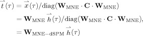
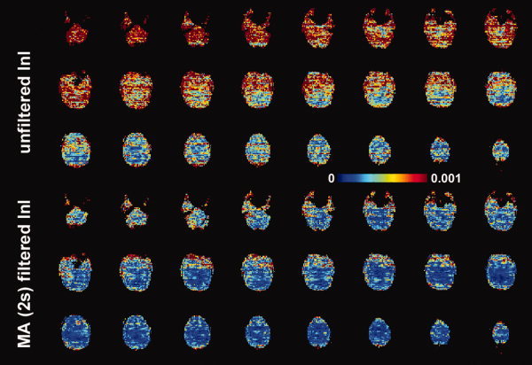
The spatial distribution of baseline noise after InI data reconstruction from a representative participant is shown in Figure 2, which includes both the unfiltered and MA (2s) filtered InI data. Plotting the noise at the same threshold for both datasets, we found a clear suppression of the baseline standard deviation across the whole brain in the filtered InI data compared with the unfiltered InI data. The baseline noise in both filtered and unfiltered data shows no distinction between the gray and white matter. This spatial distribution is similar to systematic and “non‐BOLD” physiological noise [Kruger and Glover, 2001]. We noticed that the baseline noise images were spatially blurred along the left‐right direction. This effect is because InI reconstruction uses sagittal slice projection images acquired by a 32‐channel coil array at 3T. Since the array coil has limited resolution to fully recover the spatial location in the left‐right direction, reconstructed images were calculated by using the mathematical constraint of minimizing the L2 norm of the reconstruction. Accordingly, spatial resolution was compromised in the left‐right direction. Figure 3 shows the spatial distribution of oscillatory signals around cardiac (0.9 Hz to 1.2 Hz) and respiratory (0.2 Hz to 0.4 Hz) frequencies before and after MA (2 s) filtering from one four‐minute run. Clear blurring along the left‐right direction was found, potentially due to the reduced spatial resolution in InI reconstruction as described above. There were stronger signals around the periphery of the brain in both cardiac and respiratory frequency ranges. After MA (2s) filtering, clear suppression of oscillatory signals were observed in the cardiac and respiratory frequency ranges. Specifically, the average absolute values of the unfiltered InI data in the cardiac and respiratory frequencies were 2.2 × 10⁻³ and 7.6 × 10⁻³ respectively. After applying the MA (2s) filtering, the average absolute values of the filtered InI data in the cardiac and respiratory frequencies were 0.1 × 10⁻³ and 2.2 × 10⁻³ respectively. This amounted to 15 fold and 3.4 fold suppression in the cardiac and respiratory frequencies respectively. Table I lists the baseline noise standard deviation averaged across the whole cortical surface or visual cortex in the group average. Results with and without normalization with respect to the average signal are reported. Regardless of normalization, data filtered with MA (2s) filter gave the lowest baseline variance across the whole brain. We noticed that the baseline variance was higher in the MA (3s) and MA (5s) filtered data. Note that different temporal whitening by distinct AR models was applied to the time series to ensure efficient estimation of hemodynamic responses with correct degrees of freedom. This step is likely to generate different estimates of baseline noise variance. In addition, using a long smoothing window may temporally smear the BOLD signal into baseline time points and consequently lead to over estimation of baseline fluctuation. Since baseline noise was not estimated from the moving average of unfiltered hemodynamic response, we did not observe a monotonic decrease of baseline variance.

Figure 2.

The spatial distribution of baseline noise estimated from the residuals in the GLM model. Axial slice images are shown without filtering and with MA (2 s) filtering. The color encodes the standard deviation of the noise in arbitrary units. [Color figure can be viewed in the online issue, which is available at wileyonlinelibrary.com.]

Figure 3.

The spatial distribution of noise in cardiac (0.9–1.2 Hz) and respiratory (0.2–0.4 Hz) frequency ranges. Axial slice images are shown without filtering and with MA (2 s) filtering. The color encodes the standard deviation of the noise in arbitrary units. [Color figure can be viewed in the online issue, which is available at wileyonlinelibrary.com.]

Table I.

Baseline standard deviation of the InI data with and without normalization to the average signal averaged across the entire cortex and within the visual cortex in the group analysis

		Unfiltered	MA (0.5 s)	MA (1.5 s)	MA (2 s)	MA (3 s)	MA (5 s)
Without normalization	Entire cortex (×10−5)	9.7	6.4	4.2	3.8	4.5	6.7
	Visual cortex (×10−5)	12.0	8.9	4.9	4.2	5.3	8.5
With normalization	Entire cortex (×10−3)	12.4	8.3	5.3	4.8	5.8	8.6
	Visual cortex (×10−3)	11.5	9.6	5.3	4.3	5.7	9.6

Figure 4 shows the snapshots of unfiltered InI data and 2 s MA filtered InI data from a representative participant. These snapshots show dynamic activation of the visual cortex with reasonable localization. 2 s MA filtered InI shows higher z statistics. Interestingly the 2 s MA filtered InI results show subcortical activity with dynamics similar to cortical BOLD responses. This may be the mis‐localized hemodynamic response at the lateral geniculate nucleus due to highly ill‐conditioned encoding matrix at the deep brain area.

Figure 4.

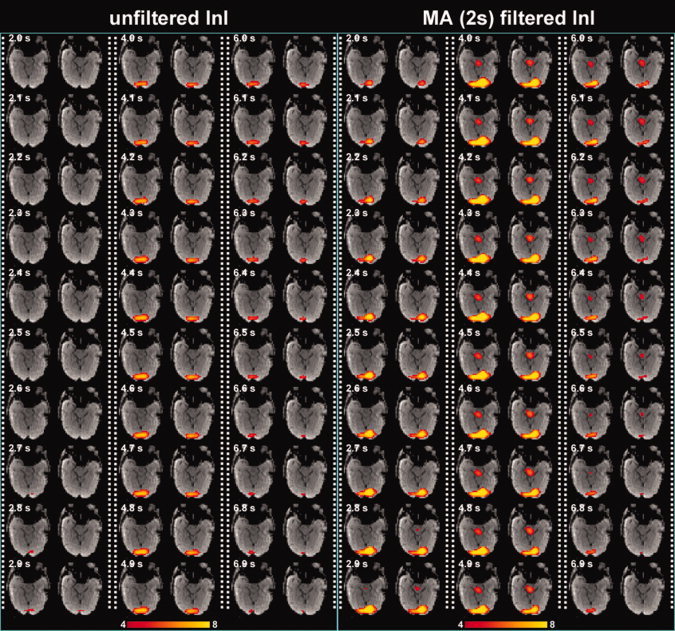
Time series of the volumetric reconstruction of unfiltered InI and filtered InI using a MA 2s filter from a representative participant. The critical threshold was z = 4. [Color figure can be viewed in the online issue, which is available at wileyonlinelibrary.com.]

The visual cortex HRFs for unfiltered InI data, 2 s MA filtered InI data, and spatially smoothed EPI (FWHM = 8.6 mm) data from a representative participant and the entire group are in Figure 5. The visual cortex average time course reaches its peak value about the same time in the unfiltered InI, filtered InI, and smoothed EPI data. Although the peak latencies vary between EPI and InI data. it is difficult to make strong inferences about these differences, due to the temporal resolution difference between EPI (TR = 2 s) and InI (TR = 0.1 s) acquisitions,. Compared to the unfiltered InI data and smoothed EPI data, we found that MA filtering of the InI data improved the detection sensitivity, as evidenced by a higher z‐statistic peak value in the visual cortex. For the single participant and the group average, MA (2s) low‐pass filtered InI results have higher peak z‐statistic values of 39.5 and 34.3 compared to either the unfiltered InI data with peak values of 17.5 and 21.8 or the smoothed EPI data with peak values of 25.1 and 21.7. Compared to unfiltered InI and spatially smoothed EPI (FWHM = 8.6 mm), MA (2 s) filtering improved the peak z‐statistics by 126% and 57% for this representative participant and 57% and 58% for the group. The InI and EPI peak values in the visual cortex for each participant and the group average are listed in Tables II and III.

Figure 5.

The average time course for a representative participant (left) and the group (right) in the visual cortex before (black trace) and after (blue trace) filtering using a MA (2 s) filter. EPI time courses (red traces) are shown for comparison. [Color figure can be viewed in the online issue, which is available at wileyonlinelibrary.com.]

Table II.

InI peak z‐statistics in the visual cortex before and after moving‐average filtering

Participant	Unfiltered InI	Temporally filtered InI
		MA (0.5s)	MA (1.5s)	MA (2s)	MA (3s)	MA (5s)
1	17.5	25.1	26.7	39.5	21.5	22.0
2	10.1	5.8	7.2	9.3	5.8	2.6
3	9.1	8.8	9.0	11.2	7.9	6.6
4	5.8	5.0	12.0	13.8	11.7	8.3
5	14.8	8.7	13.0	23.1	15.6	13.2
6	9.8	12.4	15.3	15.7	14.6	11.1
Average	21.8	18.7	29.1	34.3	25.3	17.4

Table III.

EPI peak z‐statistics in the visual cortex before and after spatial smoothing

Participant	Unsmoothed EPI	Spatially smoothed EPI
		FWHM.3.0 mm	FWHM 4.7 mm	FWHM 8.6 mm	FWHM 12 mm	FWHM 18 mm
1	9.2	9.9	14.3	25.1	18.9	20.8
2	10.7	14.3	22.4	34.3	18.1	16.2
3	8.2	8.5	10.9	11.3	6.3	5.2
4	7.4	8.8	8.7	10.1	2.9	2.1
5	12.6	13.2	16.7	20.0	18,3	17.9
6	1.9	2.2	1.9	2.2	2.1	2.1
Average	4.5	14.8	15.8	21.7	12.6	11.9

Figure 6 shows the spatial distribution of the z‐statistics averaged between 3 and 7 s after stimulus onset from a representative participant and the group average. For comparison, the EPI data spatially smoothed by a FWHM = 8.6 mm kernel are also shown rendered on the inflated cortical surfaces. The location of visual cortex is well matched in the unfiltered InI, filtered InI, and smoothed EPI conditions. Compared with the original InI data, applying a MA (2 s) filter increased the visual cortex peak z‐statistic in both the single participant and the group average (Tables II and III).

Figure 6.

A medial view of the inflated left hemisphere cortex overlaid with the z‐statistic maps showing the spatial distribution of the active visual cortex before and after MA (2 s) filtering compared to the EPI data smoothed with a 8.6 mm FWHM kernel in single participant (top panel) and group (bottom panel). The dark and light gray indicate sulci and gyri, respectively. [Color figure can be viewed in the online issue, which is available at wileyonlinelibrary.com.]

Snapshots of visual cortex activity for the group average data are shown in Figure 7. Greater spatial extent and increased task‐related activity duration were seen in the filtered InI data. Compared with the filtered InI data using a MA (2 s) filter with a z = 5 critical threshold, a later detection of suprathreshold activity was observed in the absence of filtering. Unfiltered InI data showed the suprathreshold visual cortex activity at approximately 2.3 s after the visual stimulus onset, while filtered InI data using a MA (2 s) filter showed the suprathreshold visual cortex activity at ∼ 1.7 s after the visual stimulus onset. The localization of the visual cortex, however, is very consistent between filtered and unfiltered InI data.

Figure 7.

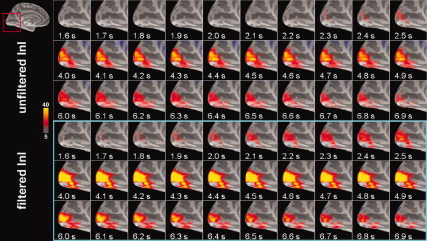
Time series of unfiltered and filtered InI cortical activity reconstructions in the visual cortex in response to visual stimulation from a group of six participants. The critical threshold was z = 5. [Color figure can be viewed in the online issue, which is available at wileyonlinelibrary.com.]

The MA (2 s) low‐pass filter was originally chosen to match TRs commonly used in multi‐slice EPI acquisition. We expected variations in the moving average filter durations to influence detection sensitivity. The results of the group z‐statistic average time courses in visual cortex are shown in Figure 8. We found that the task‐related activity peaks progressively increase when the moving average filter window increases from 0.5 s to 2 s. Further increases in the filter window decrease the observed effects. This pattern has two likely explanations. First, the failure of a short moving average window to effectively suppress oscillatory fluctuations, such as cardiac artifacts, may result in decreased contrast‐to‐noise ratios and consequent reduced sensitivity to task‐related activity. Second, a longer moving average window can suppress not only cardiac and respiratory fluctuations but also functional contrast. Thus, an excessively long moving average window can result in an overall CNR decrease. We observed small peak latency differences between hemodynamic responses estimated from filtered InI data compared to estimates derived from unfiltered InI data or EPI data. This effect may be due to differential temporally whitening associated with different AR models employed in order to achieve efficient estimation of hemodynamic responses with the correct degrees of freedom. This step is likely to effect the estimated hemodynamic response shapes and to lead to different observed latencies.

Figure 8.

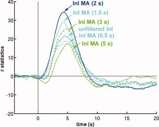
The averaged z‐statistic time course in the visual cortex using unfiltered InI data (solid cyan) and InI data filtered by different moving average filters. InI data filtered with the MA (2 s) filter (solid blue) results in the maximal peak z‐statistic value. [Color figure can be viewed in the online issue, which is available at wileyonlinelibrary.com.]

Since InI has anisotropic spatial resolution [Lin et al., 2008a; Lin et al., 2008b], we also compared filtered InI data and spatially smoothed EPI data using different smoothing kernels (Fig. 9). Compared to unsmoothed EPI data, smoothing the EPI data using kernels of FWHM = 3 mm and FWHM = 4.7 mm resulted in increased sensitivity to visual cortex activity. The largest peak statistics were found after smoothing EPI data using a kernel of FWHM = 8.6 mm. Further increasing the width of the smoothing kernel to 12 or 18 mm reduces the detection sensitivity. However, temporally filtered InI data using a MA (2 s) filter has a peak z‐ statistic of 34.3, while the highest peak z‐statistic in the spatially smoothed EPI data resulting from application of a FWHM = 8.6 mm kernel of was only 21.7 (Tables II and 3).

Figure 9.

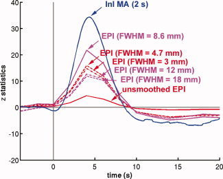
The averaged z‐statistic time course in the visual cortex using smoothed EPI data (solid red) and EPI data spatially smoothed by kernels with different widths. Among all EPI data, EPI smoothed by a kernel FWHM = 8.6 mm (solid magenta) has the maximal peak z‐statistic value. InI data filtered with the MA (2 s) filter (solid blue) has a even larger peak z‐statistic. [Color figure can be viewed in the online issue, which is available at wileyonlinelibrary.com.]

DISCUSSION

BOLD‐contrast magnetic resonance inverse imaging allows indirect detection of neural activity changes, with an order‐of‐magnitude advantage in temporal resolution when compared to standard EPI methods for whole‐brain studies. In addition to its ability to identify the fine temporal features of the hemodynamic response, InI allows use of digital processing methods for suppressing physiological noise sources without the need for external physiological monitoring devices. In the group average data, the baseline standard deviation in visual cortex in the temporally filtered InI data with a MA (2 s) filter is 39% of the unfiltered InI data (Fig. 2 and Table I). In visual cortex, the baseline standard deviation in the temporally filtered InI data with a MA (2 s) filter is 35% of the unfiltered InI data (Fig. 2 and Table I). The maximal z‐statistic in visual cortex increased from 21.8 in the unfiltered InI data to 34.3 in the filtered InI data (MA (2 s) filter, a 57% increase (Fig. 3, Tables II and III). Compared to spatially smoothed EPI data (FWHM = 8.6 mm), the filtered InI data has a 58% higher peak z‐value (Fig. 3, Tables II and III). This result is higher than the 4% increase observed when using adaptive filtering, which has comparable performance to that seen with the RETROICOR method [Deckers et al., 2006]. The advantages InI provides in suppressing physiological noise include increased detection sensitivity in all InI fMRI experiments. Our filtering approach can also aid in detecting subtle changes in response timing within brain areas across task conditions. When comparing timing differences at a particular brain location, there are no confounding influences contributed by differential vasculature effects and therefore the timing difference between conditions can more easily be attributed to changes in neural activity.

In contrast to many previously described techniques for reducing the effects of physiological noise, InI filtering does not require an external cardiac or respiratory monitoring device to directly record cardiac and respiratory activity that, when undersampled in the temporal domain, can lead to aliased noised. External monitoring devices can collect cardiac and respiratory signals that can be used to create nuisance‐variable regressors [Birn et al., 2006; Lund et al., 2006] to remove periodic, low‐frequency (<0.1 Hz) sources of physiological noise. However, there is an unknown latency between these peripherally monitored signals and their associated brain signals. The peripheral to central latency can also vary due to spatial variations in neurovascular coupling. Physiologically, pulsations of cardiac or respiratory origin have dominant frequencies around 1.0 and 0.25 Hz respectively. Both noise sources are relatively broadband because of the intrinsic variability in autonomic nervous system modulation and the mutual interaction between the competing sympathetic and parasympathetic influences. Using standard EPI acquisition techniques, while it is possible to monitor and subsequently reduce low‐frequency (<0.1 Hz) CO₂‐mediated physiological noise [Birn et al., 2006; Shmueli et al., 2007; Wise et al., 2004], it is more difficult to remove the effects of respiratory and cardiac fluctuations due to sampling rate limitations. While it usually takes up to 2 s to complete an EPI volumetric acquisition with whole‐brain coverage, the required sampling period to avoid cardiac noise aliasing based on the Nyquist sampling theorem is 0.5 s or less. InI can avoid this problem by achieving whole‐brain acquisition with sampling intervals as short as 0.1 s using RF encoding.

Because of the ill‐posed nature of raw InI data, there exist different alternatives for InI image reconstruction, including minimum L2 norm [Lin et al., 2008a], spatial filtering [Lin et al., 2008b], or k‐space techniques [Lin et al., 2010]. However, the utility of the filtering method examined in this paper is not dependent on any specific image reconstruction algorithm. Physiological noise can first be suppressed using digital filtering, after which a particular reconstruction algorithm can be chosen. Therefore, digital filtering can be considered as a pre‐processing step with benefits independent of particular reconstruction methods.

In this study, we used temporal filters to reduce the effects of cardiac and respiratory noise. While other digital filtering techniques can be used to suppress these noise sources, moving average filters are computationally efficient and extremely easy to implement. Theoretically, the use of MA filters can result in passband ringing. However, our results did not show significant ringing artifacts in the spectral (Fig. 1) or temporal (Fig. 5) domains. One disadvantage of employing a moving average filter is that the low‐pass filtering does indeed increase the temporal correlation among the elements of a time series. Therefore, studies concerned with very transient fMRI responses may therefore benefit from the use of other filtering methods to reduce cardiac and respiratory noise without distorting the fine temporal structure of the task‐related responses. For example, adaptive filtering methods have been applied in optical imaging to reduce global signal variation [Zhang et al., 2007]. In theory, these methods can be applied to InI data to reduce physiological noise while preserving the temporal structure of transient signal changes.

The physiological noise sources that have been the focus of our study mostly originate from cyclic cardiac and respiratory activity. We assume that these artifacts have quasi‐periodic waveforms and that the sampling rate of volumetric inverse imaging is sufficiently fast to avoid temporal noise aliasing. The current implementation of volumetric InI uses 100 ms temporal resolution for whole‐brain coverage. This sampling frequency, in typical physiological conditions, is sufficiently high to meet the Nyquist sampling criterion. The cost associated with the high InI sampling rate is a loss of spatial resolution, since InI solves underdetermined linear systems in image reconstructions. Due to the ill posed nature of these underdetermined linear systems, there exist an infinite number of solutions. However, imposing constraints can allow solution of underdetermined linear systems. We previously investigated the use of minimum L2 norm solutions [Lin et al., 2008a] and spatial filtering techniques using linear constraint minimum variance beamformers [Lin et al., 2008b]. Depending on the SNR of the measurements, it is possible to obtain an average point spread function of 8.6, 4.7, and 3.0 mm in minimum L2 norm reconstructions at SNRs of 10, 5, and 1, respectively. Since fMRI data collected using EPI acquisition methods usually involves spatial smoothing to improve the SNR [Friston, 2007], a small loss of spatial resolution is generally considered acceptable. Note that if the LCMV beamformer is used as an alternative reconstruction algorithm for InI data, the average point spread function is usually below 1 mm [Lin et al., 2008b]. In this case, the loss of spatial resolution may be negligible.

We found that Figures 2, 3, and 4 were not perfectly symmetric along the left‐right direction. Note that these figures are results of functional activity rather than anatomy. Thus we cannot completely attribute asymmetric appearance to the reconstruction. Notably, Figure 4 is the result from one single subject. And there have been reports on the variability of visual cortex BOLD responses [de Zwart et al., 2005; Handwerker et al., 2004], which might explain why the observed visual cortex activity is not 100% symmetric even symmetric stimuli were presented.

InI indeed has intrinsic a spatial smoothing effect as the result of using the constraint of minimizing the L‐2 norm of the reconstruction. Such smoothing can improve the signal‐to‐noise ratio and it is spatially variying [Lin et al., 2010; Lin et al., 2008a; Lin et al., 2008b]. Considering the common EPI processing stream using only one homogeneous 3D smoothing kernel, a fair comparison, in our mind, would be spatially smoothing InI and EPI such that the average cortical resolution is comparable. This is in fact what we did. Even considering different spatial smoothing effects in InI reconstructions, Figure 8 clearly shows that EPI data using different spatially smoothing kernels (FWHM = 3 mm to 18 mm) do not generate as high statistics as temporally smoothed InI data. Taken together, spatial smoothing in InI is not dominating the SNR improvement in BOLD fMRI time series. The suppression of the fluctuation in InI time also contributes significantly to the overall improvement in the sensitivity of BOLD hemoydnamic responses detection.

Cardiac and respiratory periodic modulations are part of the “non‐BOLD” component of physiological temporal noise (σ_NB) [Kruger and Glover, 2001]. The other type of physiological temporal noise is similar to BOLD‐contrast signal (σ_B), whose magnitude depends on TE of the measurement [Kruger and Glover, 2001]. σ_NB noise has a more homogenous spatial distribution, while σ_B noise is higher in gray matter than white matter [Kruger and Glover, 2001]. With TR = 3 s, the ratio between σ_NB and σ_B noise at 3T is ∼ 1:2, implying that our temporal filtering method can optimally reduce physiological noise by 33%. Note that these numbers depend on TE, flip angle [Gonzalez‐Castillo, 2010], and TR. To further reduce the σ_B physiological noise, we may look to other solutions. It has been suggested that sampling with high spatial resolution and subsequently smoothing the data along the gray matter can effectively reduce the σ_B physiological noise [Triantafyllou et al., 2006]. This is due to the fact that physiological noise sources are partially spatially correlated. Sampling at higher spatial resolution can ensure that the noise sources are dominated by thermal, rather than physiological, noise. Subsequent spatial smoothing of thermal noise dominated data can compensate for the loss of signal without lowering the SNR, since thermal noise is spatially uncorrelated. Increasing spatial resolution to reduce the relative contribution of physiological noise reduces the advantage of InI as compared with EPI. However, if we know a priori that the σ_B noise is less concentrated in a specific k‐space region, as suggested by [Bodurka et al., 2007; Lowe and Sorenson, 1997], then InI accelerated scans can be acquired in that specific k‐space region in order to reduce physiological noise contamination. Namely, instead of acquiring projection images (k _z = 0) in InI, we can also acquire k‐space data corresponding to a spatial harmonic (k _z ≠ 0) in accelerated InI acquisition. Hypothetically, the reconstructed volumetric images can have reduced physiological noise.

It has been suggested that a steady state free precession (SSFP) signal can develop under a train of RF pulses with TR < T2 in single‐shot EPI [Zhao et al., 2000]. B₀ fluctuations originating from respiration, physical movement outside the FOV, and system instability can cause SSFP temporal variation. InI uses a brief TR = 100 ms and thus this mechanism can potentially contribute to time series variation. It has been suggested that a strong crusher can be used to minimize these temporal noise fluctuations [Zhao et al., 2000]. In fact, our experiment used a crusher gradient of 20 mT/m strength and 10‐ms duration, as previously suggested [Zhao et al., 2000]. However, since the suggested strong crusher was studied with TR = 200 ms, InI may require further increase the crusher moment to reduce the SSFP signal disturbance by increasing the crusher duration or strength. However, the potential cost will be reduced temporal resolution and more prominent eddy current artifacts.

In conclusion, the high sampling rate made possible with MR InI can be exploited to monitor and suppress cardiac and respiratory physiological noise sources without the need for external monitoring devices. We systematically investigated this advantage by parametrically modulating the temporal filtering parameters and then comparing the results to EPI acquisitions processed with different spatial smoothing kernels. The improved detection power after physiological noise suppression was validated across participants and the improvements resulting from noise suppression are strong and statistically significant. The InI method can be used in BOLD‐contrast fMRI experiments using parallel detection from a RF coil array to further improve the sensitivity of detecting localized changes in neural activity that are either spontaneous, as in resting state studies, or task‐related, as in investigations of the neural mechanisms of perception, cognition and action.

REFERENCES

- Barry RL, Menon RS ( 2005): Modeling and suppression of respiration‐related physiological noise in echo‐planar functional magnetic resonance imaging using global and one‐dimensional navigator echo correction. Magn Reson Med 54: 411–418. [DOI] [PubMed] [Google Scholar]
- Birn RM, Diamond JB, Smith MA, Bandettini PA ( 2006): Separating respiratory‐variation‐related fluctuations from neuronal‐activity‐related fluctuations in fMRI. Neuroimage 31: 1536–1548. [DOI] [PubMed] [Google Scholar]
- Biswal B, DeYoe AE, Hyde JS ( 1996): Reduction of physiological fluctuations in fMRI using digital filters. Magn Reson Med 35: 107–113. [DOI] [PubMed] [Google Scholar]
- Bodurka J, Ye F, Petridou N, Murphy K, Bandettini PA ( 2007): Mapping the MRI voxel volume in which thermal noise matches physiological noise–implications for fMRI. Neuroimage 34: 542–549. [DOI] [PMC free article] [PubMed] [Google Scholar]
- Brainard DH ( 1997): The Psychophysics Toolbox. Spat Vis 10( 4), 433–436. [PubMed] [Google Scholar]
- Cox RW, Jesmanowicz A ( 1999): Real‐time 3D image registration for functional MRI. Magn Reson Med 42: 1014–1018. [DOI] [PubMed] [Google Scholar]
- Dagli MS, Ingeholm JE, Haxby JV ( 1999): Localization of cardiac‐induced signal change in fMRI. Neuroimage 9: 407–415. [DOI] [PubMed] [Google Scholar]
- Dale AM, Fischl B, Sereno MI ( 1999): Cortical surface‐based analysis. I. Segmentation and surface reconstruction. Neuroimage 9: 179–194. [DOI] [PubMed] [Google Scholar]
- Dale AM, Liu AK, Fischl BR, Buckner RL, Belliveau JW, Lewine JD, Halgren E ( 2000): Dynamic statistical parametric mapping: Combining fMRI and MEG for high‐resolution imaging of cortical activity. Neuron 26: 55–67. [DOI] [PubMed] [Google Scholar]
- de Zwart JA, Silva AC, van Gelderen P, Kellman P, Fukunaga M, Chu R, Koretsky AP, Frank JA, Duyn JH ( 2005): Temporal dynamics of the BOLD fMRI impulse response. Neuroimage 24: 667–677. [DOI] [PubMed] [Google Scholar]
- Deckers RH, van Gelderen P, Ries M, Barret O, Duyn JH, Ikonomidou VN, Fukunaga M, Glover GH, de Zwart JA ( 2006): An adaptive filter for suppression of cardiac and respiratory noise in MRI time series data. Neuroimage 33: 1072–1081. [DOI] [PMC free article] [PubMed] [Google Scholar]
- Feinberg DA ( 1992): Modern concepts of brain motion and cerebrospinal fluid flow. Radiology 185: 630–632. [DOI] [PubMed] [Google Scholar]
- Feinberg DA, Mark AS ( 1987): Human brain motion and cerebrospinal fluid circulation demonstrated with MR velocity imaging. Radiology 163: 793–799. [DOI] [PubMed] [Google Scholar]
- Fischl B, Sereno MI, Dale AM. ( 1999a): Cortical surface‐based analysis. II: Inflation, flattening, and a surface‐based coordinate system. Neuroimage 9: 195–207. [DOI] [PubMed] [Google Scholar]
- Fischl B, Sereno MI, Tootell RB, Dale AM. ( 1999b): High‐resolution intersubject averaging and a coordinate system for the cortical surface. Hum Brain Mapp 8: 272–284. [DOI] [PMC free article] [PubMed] [Google Scholar]
- Friston KJ. 2007. Statistical Parametric Mapping: The Analysis of Funtional Brain Images. Amsterdam: Boston: Elsevier/Academic Press; vii, 647 p. [Google Scholar]
- Glover GH ( 1999): Deconvolution of impulse response in event‐related BOLD fMRI. Neuroimage 9: 416–429. [DOI] [PubMed] [Google Scholar]
- Glover GH, Li TQ, Ress D ( 2000): Image‐based method for retrospective correction of physiological motion effects in fMRI: RETROICOR. Magn Reson Med 44: 162–167. [DOI] [PubMed] [Google Scholar]
- Gonzalez‐Castillo J, Roopchansingh V, Bandettini PA, Bodurka J ( 2010): Physiological noise effects on the flip angle selection in BOLD fMRI. Neuroimage 54: 2764–2778. [DOI] [PMC free article] [PubMed] [Google Scholar]
- Hajnal JV, Myers R, Oatridge A, Schwieso JE, Young IR, Bydder GM ( 1994): Artifacts due to stimulus correlated motion in functional imaging of the brain. Magn Reson Med 31: 283–291. [DOI] [PubMed] [Google Scholar]
- Handwerker DA, Ollinger JM, D'Esposito M ( 2004): Variation of BOLD hemodynamic responses across subjects and brain regions and their effects on statistical analyses. Neuroimage 21: 1639–1651. [DOI] [PubMed] [Google Scholar]
- Hennig J, Zhong K, Speck O ( 2007): MR‐Encephalography: Fast multi‐channel monitoring of brain physiology with magnetic resonance. Neuroimage 34: 212–219. [DOI] [PubMed] [Google Scholar]
- Hu X, Kim SG ( 1994): Reduction of signal fluctuation in functional MRI using navigator echoes. Magn Reson Med 31: 495–503. [DOI] [PubMed] [Google Scholar]
- Hu X, Le TH, Parrish T, Erhard P ( 1995): Retrospective estimation and correction of physiological fluctuation in functional MRI. Magn Reson Med 34: 201–212. [DOI] [PubMed] [Google Scholar]
- Kruger G, Glover GH ( 2001): Physiological noise in oxygenation‐sensitive magnetic resonance imaging. Magn Reson Med 46: 631–637. [DOI] [PubMed] [Google Scholar]
- Kwong KK, Belliveau JW, Chesler DA, Goldberg IE, Weisskoff RM, Poncelet BP, Kennedy DN, Hoppel BE, Cohen MS, Turner R, et al. ( 1992): Dynamic magnetic resonance imaging of human brain activity during primary sensory stimulation. Proc Natl Acad Sci USA 89: 5675–5679. [DOI] [PMC free article] [PubMed] [Google Scholar]
- Lin FH, Wald LL, Ahlfors SP, Hamalainen MS, Kwong KK, Belliveau JW ( 2006): Dynamic magnetic resonance inverse imaging of human brain function. Magn Reson Med 56: 787–802. [DOI] [PubMed] [Google Scholar]
- Lin FH, Witzel T, Chang WT, Wen‐Kai Tsai K, Wang YH, Kuo WJ, Belliveau JW ( 2010): K‐space reconstruction of magnetic resonance inverse imaging (K‐InI) of human visuomotor systems. Neuroimage 49: 3086–3098. [DOI] [PMC free article] [PubMed] [Google Scholar]
- Lin FH, Witzel T, Mandeville JB, Polimeni JR, Zeffiro TA, Greve DN, Wiggins G, Wald LL, Belliveau JW ( 2008a): Event‐related single‐shot volumetric functional magnetic resonance inverse imaging of visual processing. Neuroimage 42: 230–247. [DOI] [PMC free article] [PubMed] [Google Scholar]
- Lin FH, Witzel T, Zeffiro TA, Belliveau JW ( 2008b): Linear constraint minimum variance beamformer functional magnetic resonance inverse imaging. Neuroimage 43: 297–311. [DOI] [PMC free article] [PubMed] [Google Scholar]
- Logothetis NK, Pauls J, Augath M, Trinath T, Oeltermann A ( 2001): Neurophysiological investigation of the basis of the fMRI signal. Nature 412: 150–157. [DOI] [PubMed] [Google Scholar]
- Lowe MJ, Sorenson JA ( 1997): Spatially filtering functional magnetic resonance imaging data. Magn Reson Med 37: 723–729. [DOI] [PubMed] [Google Scholar]
- Lund TE, Madsen KH, Sidaros K, Luo WL, Nichols TE ( 2006): Non‐white noise in fMRI: Does modelling have an impact? Neuroimage 29: 54–66. [DOI] [PubMed] [Google Scholar]
- McDougall MP, Wright SM ( 2005): 64‐channel array coil for single echo acquisition magnetic resonance imaging. Magn Reson Med 54: 386–392. [DOI] [PubMed] [Google Scholar]
- Mistretta CA, Wieben O, Velikina J, Block W, Perry J, Wu Y, Johnson K, Wu Y ( 2006): Highly constrained backprojection for time‐resolved MRI. Magn Reson Med 55: 30–40. [DOI] [PMC free article] [PubMed] [Google Scholar]
- Mitra PP, Pesaran B ( 1999): Analysis of dynamic brain imaging data. Biophys J 76: 691–708. [DOI] [PMC free article] [PubMed] [Google Scholar]
- Neumaier A, Schneider T ( 2001): Estimation of parameters and eigenmodes of multivariate autoregressive models. ACM Trans. Math Softw 27: 27–57. [Google Scholar]
- Ogawa S, Lee TM, Kay AR, Tank DW ( 1990): Brain magnetic resonance imaging with contrast dependent on blood oxygenation. Proc Natl Acad Sci USA 87: 9868–9872. [DOI] [PMC free article] [PubMed] [Google Scholar]
- Pelli DG ( 1997): The VideoToolbox software for visual psychophysics: transforming numbers into movies. Spat Vis 10: 437–442. [PubMed] [Google Scholar]
- Percival DB, Walden AT ( 1993): Spectral Analysis for Physical Applications: Multitaper and Conventional Univariate Techniques. Cambridge, New York, NY: Cambridge University Press; xxvii, 583 p. [Google Scholar]
- Pfeuffer J, Van de Moortele PF, Ugurbil K, Hu X, Glover GH ( 2002): Correction of physiologically induced global off‐resonance effects in dynamic echo‐planar and spiral functional imaging. Magn Reson Med 47: 344–353. [DOI] [PubMed] [Google Scholar]
- Poncelet BP, Wedeen VJ, Weisskoff RM, Cohen MS ( 1992): Brain parenchyma motion: Measurement with cine echo‐planar MR imaging. Radiology 185: 645–651. [DOI] [PubMed] [Google Scholar]
- Pruessmann KP, Weiger M, Scheidegger MB, Boesiger P ( 1999): SENSE: Sensitivity encoding for fast MRI. Magn Reson Med 42: 952–962. [PubMed] [Google Scholar]
- Purdon PL, Weisskoff RM ( 1998): Effect of temporal autocorrelation due to physiological noise and stimulus paradigm on voxel‐level false‐positive rates in fMRI. Hum Brain Mapp 6: 239–249. [DOI] [PMC free article] [PubMed] [Google Scholar]
- Schneider T, Neumaier A ( 2001): Algorithm 808: ARfit ‐ A Matlab package for the estimation of parameters and eigenmodes of multivariate autoregressive models. ACM Trans Math Softw 27: 58–65. [Google Scholar]
- Shmueli K, van Gelderen P, de Zwart JA, Horovitz SG, Fukunaga M, Jansma JM, Duyn JH ( 2007): Low‐frequency fluctuations in the cardiac rate as a source of variance in the resting‐state fMRI BOLD signal. Neuroimage 38: 306–320. [DOI] [PMC free article] [PubMed] [Google Scholar]
- Sodickson DK, Manning WJ ( 1997): Simultaneous acquisition of spatial harmonics (SMASH): Fast imaging with radiofrequency coil arrays. Magn Reson Med 38: 591–603. [DOI] [PubMed] [Google Scholar]
- Thomas CG, Harshman RA, Menon RS ( 2002): Noise reduction in BOLD‐based fMRI using component analysis. Neuroimage 17: 1521–1537. [DOI] [PubMed] [Google Scholar]
- Triantafyllou C, Hoge RD, Wald LL ( 2006): Effect of spatial smoothing on physiological noise in high‐resolution fMRI. Neuroimage 32: 551–557. [DOI] [PubMed] [Google Scholar]
- Windischberger C, Langenberger H, Sycha T, Tschernko EM, Fuchsjager‐Mayerl G, Schmetterer L, Moser E ( 2002): On the origin of respiratory artifacts in BOLD‐EPI of the human brain. Magn Reson Imaging 20: 575–582. [DOI] [PubMed] [Google Scholar]
- Wise RG, Ide K, Poulin MJ, Tracey I ( 2004): Resting fluctuations in arterial carbon dioxide induce significant low frequency variations in BOLD signal. Neuroimage 21: 1652–1664. [DOI] [PubMed] [Google Scholar]
- Woods RP, Grafton ST, Holmes CJ, Cherry SR, Mazziotta JC ( 1998): Automated image registration. I. General methods and intrasubject, intramodality validation. J Comput Assist Tomogr 22: 139–152. [DOI] [PubMed] [Google Scholar]
- Worsley KJ, Liao CH, Aston J, Petre V, Duncan GH, Morales F, Evans AC ( 2002): A general statistical analysis for fMRI data. Neuroimage 15: 1–15. [DOI] [PubMed] [Google Scholar]
- Zhang Q, Brown EN, Strangman GE. ( 2007) Adaptive filtering to reduce global interference in evoked brain activity detection: A human subject case study. J Biomed Opt 12: 064009. [DOI] [PubMed] [Google Scholar]
- Zhao X, Bodurka J, Jesmanowicz A, Li SJ ( 2000): B(0)‐fluctuation‐induced temporal variation in EPI image series due to the disturbance of steady‐state free precession. Magn Reson Med 44: 758–765. [DOI] [PubMed] [Google Scholar]