

Abstract
Attention to a spatial location or feature in a visual scene can modulate the responses of cortical neurons and affect perceptual biases in illusions. We add attention to a cortical model of spatial context based on a well-founded account of natural scene statistics. The cortical model amounts to a generalized form of divisive normalization, in which the surround is in the normalization pool of the center target only if they are considered statistically dependent. Here we propose that attention influences this computation by accentuating the neural unit activations at the attended location, and that the amount of attentional influence of the surround on the center thus depends on whether center and surround are deemed in the same normalization pool. The resulting form of model extends a recent divisive normalization model of attention (Reynolds & Heeger, 2009). We simulate cortical surround orientation experiments with attention and show that the flexible model is suitable for capturing additional data and makes nontrivial testable predictions.
Keywords: Bayesian, scene statistics, divisive normalization, visual attention
Introduction
We interpret the visual environment not only based on the bottom-up properties of the visual inputs. Top-down attention—for instance, directed to a particular location or property of the scene—also plays a critical role. Indeed, top-down attention is widely studied in visual neuroscience and psychology and has been found experimentally to influence both the response properties of cortical neurons and perception (for reviews, see Carrasco, 2011; Maunsell & Treue, 2006; Reynolds & Chelazzi, 2004). There has also been great interest in computational modeling of a wide range of attention effects (e.g., Chikkerur, Serre, Tan, & Poggio, 2010; Dayan & Solomon, 2010; Dayan & Zemel, 1999; Rao, 2005; Yu & Dayan, 2005; Yu, Dayan, & Cohen, 2009; for some recent reviews and books, see Eckstein, Peterson, Pham, & Droll, 2009; Reynolds & Heeger, 2009; Tsotsos, 2011; Whiteley, 2008).
Here we focus on the interaction between spatial context and attention in visual processing, with emphasis on orientation stimuli and cortical processing in the ventral stream. Specifically, we focus on various types of cortical neurophysiology data that have emerged. This includes data that have previously been modeled, such as changes in tuning curves due to attention (e.g., McAdams & Maunsell, 1999) and changes in response and contrast gain (e.g., Reynolds & Heeger, 2009). In addition, we consider data pertaining to the orientation, contrast, and geometrical arrangement of stimuli inside and outside the classical receptive field (e.g., Moran & Desimone, 1985; Sundberg, Mitchell, & Reynolds, 2009; Wannig, Stanisor, & Roelfsema, 2011).
From the modeling perspective, we focus on divisive normalization accounts, which are widespread in neuroscience (e.g., Carandini & Heeger, 2012; Geisler & Albrecht, 1992; Heeger, 1992). We consider two relevant sets of literature. First, cortical models have been developed based on the hypothesis that neurons are matched to the statistical properties of scenes (e.g., Attneave, 1954; Barlow, 1961; Bell & Sejnowski, 1997; Olshausen & Field, 1996; Simoncelli & Olshausen, 2001; Zhaoping, 2006). In particular, it has been shown that scene statistics models can be related to nonlinear neural computations (e.g., Karklin & Lewicki, 2009; Rao & Ballard, 1999; Zetzsche & Nuding, 2005), including divisive normalization (e.g., Coen-Cagli, Dayan, & Schwartz, 2012; Schwartz & Simoncelli, 2001). However, these approaches have thus far not incorporated attention effects (although see Spratling, 2008, for a predictive coding framework). Second, descriptive models of divisive normalization have recently been extended to include attention inside and outside the classical receptive field and have shown to impressively unify a range of cortical attention data (Ghose, 2009; Lee & Maunsell, 2009; Reynolds & Heeger, 2009). The divisive normalization signal in descriptive models is typically not constrained and includes neural units with a wide range of features such as orientations. Here, we essentially merge these two approaches, namely incorporating attention in a divisive normalization model, in which the form of the model and the normalization pools are motivated from scene statistics considerations.
More specifically, we have recently developed a cortical model of spatial context (without attention), based on a Bayesian account of natural scene statistics. The form of model amounts to a generalized divisive normalization and can address some biological data on spatial context effects (Coen-Cagli, Dayan, & Schwartz, 2009, 2012; Schwartz, Sejnowski, & Dayan, 2009). A critical aspect of the model that goes beyond canonical models of divisive normalization is the inclusion of a flexible divisive normalization pool: For a given visual input, neural units in the surround location divisively normalize the center unit, only if the center and surround are considered statistically dependent according to the model (for instance, if they have similar orientation and are considered part of a statistically homogenous texture or object). In contrast, when center and surround are thought to be statistically different, then the surround units do not normalize the response of the center unit. Here our goal is to address the influence of attention in this class of model.
We propose that attention multiplicatively accentuates the attended features and locations in the model and that Bayesian estimation then proceeds as before: The model determines the degree to which the attention-modulated center and surround are deemed statistically dependent, and divisively normalizes by the surround appropriately. This results in an influence that is equivalent to Reynolds and Heeger (2009), in which the output of a neuron is divisively normalized by a signal computed by other neurons in the normalization pool, and both the numerator and the normalization pool are modulated by attention. However, extending Reynolds and Heeger (2009), in our model there is an interplay between the normalization pools and attention. We thus put together flexible normalization pools from image statistics considerations and the influence of attention.
In the next section, we include an introduction to the main components of the modeling. This is followed by a more detailed Methods section. In the Results section, we show that the resulting flexible normalization model replicates key results of the divisive normalization model of attention given its similar form. We show that it also addresses additional cortical attention data that we suggest require more flexible divisive normalization pools and makes testable predictions for cortical surround attention experiments in which the model diverges from the canonical divisive normalization. In the Discussion section, we also discuss implications for perceptual illusion biases (in light of our previous work; Schwartz et al., 2009) in the context of attention.
Introduction to the modeling
We next describe in nontechnical terms the scene statistics approach and the relation of the statistical modeling to divisive normalization. We also address how the statistical model compares to the canonical model of divisive normalization and how we might think about the model components in neural terms.
The statistical model and divisive normalization
We adopt a model of scene statistics that is closely related to divisive normalization. The main motivation for the model comes from the empirical observation that the activations of oriented cortical-like filters to natural scenes exhibit statistical dependencies. We would like to relate these dependencies to a model of the cortical neural output. There are two main approaches. The first approach is to find a transform that makes the outputs more independent, assuming for instance that neurons aim to code the visual input more efficiently (e.g., Attneave, 1954; Barlow, 1961). It has been shown that this can be achieved through divisive normalization (e.g., Schwartz & Simoncelli, 2001).
A second related approach, which we adopt here, is to build a model that can generate the statistical dependencies between filter activations and then relate a component of this model to the neural output. This is known as a generative modeling approach (e.g., Hinton & Ghahramani, 1997). It has been shown that the dependencies of filter activations to natural scenes are well described by a multiplicative model (e.g., Wainwright & Simoncelli, 2000). For instance, to generate dependencies between two filter activations (say at two different spatial locations), one starts with two independent variables corresponding to the filters at the two locations and multiplies each of them by a common variable that introduces the dependency. We describe the cortical neural output at a given spatial location as essentially reversing this procedure and estimating its local independent variable. Since the generative model is multiplicative, this amounts to the reverse process, i.e., divisive normalization.
The advantage of the generative approach, which is common also in the broader machine learning community, is that rather than searching for a suitable transform, one can build a suitably rich model that captures the statistical dependencies and then reverse the model. In the Methods section, we formalize this process in a class of generative model known as Gaussian Scale Mixture (GSM), which we have previously applied to simulating cortical data without attention (e.g., Coen-Cagli et al., 2012). In this class of model, the cortical output of the model corresponds to Bayesian estimation of the local variable in light of the statistical dependencies. The generative modeling approach also leads to a richer model than the canonical model of divisive normalization, which we denote the flexible normalization model.
Canonical normalization, tuned normalization, and flexible normalization
In Figure 1, we provide intuition for the main modeling approach and how it compares to the canonical divisive normalization model. Figure 1b (left) shows a simplified cartoon of the canonical divisive normalization model (e.g., Heeger, 1992). In this model, the surround filter activation (and more generally, multiple surround filter activations in the normalization pool) always divisively modulates the center filter activation. From the scene statistics perspective, the division comes about via estimation in a Bayesian model in which center and surround filter activations are always assumed to be statistically dependent, as is common between spatially adjacent regions in natural scenes. The model estimates the response of a center neuron in light of these assumed dependencies. This amounts to a divisive normalization computation, which also reduces the dependencies (Schwartz & Simoncelli, 2001).
Figure 1.

Divisive normalization in the GSM model and attention. (a) Cartoon of image statistics in the GSM model. The center and surround are either statistically dependent and share a common mixer variable (green for homogenous regions of the scene, such as within the zebra) or are independent each with their own mixer variable (blue for nonhomogenous regions, such as across the zebra border). Filter activations are given by xc (for center) and xs (for surround). The cartoon shows two filters, but the model generalizes for more filters. (b) The canonical divisive normalization version of the GSM model assumes that center and surround filter activations are always dependent, and thus the center filter activation is always divided by the surround activation. The cartoon illustrates example experimental stimuli. Attention is assumed to modulate the observed filter activations in both center and surround locations multiplicatively (only surround attention shown by the red circle). Attention weights are given by ac (for center) and as (for surround). The cortical model estimates the mean firing rate corresponding to the center location via divisive normalization (formally, this is done by estimating the Gaussian component in the GSM model; see main text). This model is similar to Reynolds and Heeger (2009) but includes a tuned surround. (c) The flexible pool divisive normalization model determines the degree to which center and surround activations are deemed dependent or independent. For the dependent case, the surround is in the normalization pool of the center; for the independent case, the surround is not in the normalization pool of the center.
Another important point to note is that filter activations in two spatial locations are more statistically dependent when the center and surround orientations are similar (Schwartz & Simoncelli, 2001). For this reason, one straightforward version of the canonical model that we will adopt here is a tuned divisive normalization model, i.e., we assume that filters in the center and surround locations have a similar orientation (Schwartz et al., 2009). In Figure 1b (right) we also show the canonical divisive normalization model with attention (Reynolds & Heeger, 2009), whereby filter activations in both center and surround are multiplicatively weighted by attention prior to divisive normalization. The statistical version turns out equivalent: Attention is assumed to multiplicatively weight center and surround filter activations; center and surround activations modulated by attention are still always assumed dependent, and the division proceeds appropriately for the Bayesian estimation of the center component. We note further that in most model simulations, we assume for simplicity that all surround locations are weighted equally in their contribution to divisive normalization (as in Schwartz et al., 2009). In one of the simulations addressing geometric influences of surround normalization with attention, we relax this assumption (as in Coen-Cagli et al., 2009, 2012), and allow nonequal weighting of different spatial positions in the surround.
Second, we consider an extension of the model to flexible divisive normalization. In the flexible pool divisive normalization model, we assume a richer and more correct model of scene statistics (Schwartz et al., 2009), in which center and surround could either be deemed statistically dependent (as is common in homogenous regions of an image or within objects), or statistically independent (as is common across objects with different statistics; see Figure 1a). This results in a neural model in which the surround activations divide the center to the degree that they are deemed statistically dependent according to the model (Figure 1c, left). In our model, the normalization pools (which include either normalization by the center or normalization by both center and surround) and the priors for each of the pools are set in advance. The degree to which each of the divisive normalization pools contribute to the neural output (i.e., the posterior probability for each of the pools) is then computed via Bayesian inference, given the filter activations to the input stimuli. In this way, when the center and surround stimuli are more similar (for instance in contrast and orientation), they are deemed more dependent according to the model, and the surround normalizes the center, but when center and surround stimuli are very different, the surround does not normalize the center. We also show the flexible normalization model with attention (Figure 1c, right): Now the Bayesian model determines the degree to which the attention-modulated center and surround activations are deemed dependent and normalizes appropriately.
Potential neural correlates of the flexible normalization
Before proceeding to a more detailed description of the modeling, we describe intuitively how one might think about the model components in neural terms. It is important to note that divisive normalization has indeed been termed a canonical neural computation (Carandini & Heeger, 2012), for which there are many possible neural correlates. In the context of surround effects which is our main focus here, it has been suggested that divisive normalization might be mediated by feedback from higher areas (e.g., terminating on inhibitory interneurons) and horizontal connections, both of which have been suggested to be orientation dependent.
The extension to a flexible normalization model requires a mechanism whereby the divisive signal is not fixed but can vary with the input stimuli. Although nailing down the mechanisms is a task for future work, we note several possibilities here (see also discussion and references in Coen-Cagli et al., 2012). One possibility is that the stimulus dependence might arise through the diversity of the interneurons that mediate divisive normalization. The group of interneurons and their properties (e.g., their selectivity and firing threshold) might be set in advance (as for the normalization pools and priors in our model). However, the flexibility could arise because different input stimuli could turn on or off the interneurons to different degrees (Moore, Carlen, Knoblich, & Cardin, 2010), and this could depend on aspects such as contrast or attention (as for the Bayesian inference in our model). Alternatively, the flexible normalization might be an emergent property of the network dynamics—for instance, through stimulus-dependent changes in the effectiveness of lateral connections (Nauhaus, Busse, Carandini, & Ringach, 2009) or through switching between network regimes (Salinas, 2003) or dynamic stabilization of the neural network (Ahmadian, Rubin, & Miller, 2012).
The role of attention
The attention model assumes that the priors for the normalization pools are determined from natural scenes and that attention acts given the priors from scenes. We think that a main benefit of attention within this framework is that it acts as a more reliable cue to improve local estimates due to shared dependency. That is, if one attends to a surround location, it should only influence the center computation and contribute to divisive normalization in as much as the center and surround are believed to be statistically dependent (if center and surround are independent, there is no need to use the surround information in estimating the center). One should properly take account of these dependencies inherent in natural scene statistics also in the face of attention. Our framework therefore ties together so-called normative/functional scene statistics approaches, with the attention model of Reynolds and Heeger (2009). Note, however, that we think pinning down the functional benefits of attention would require a formal treatment of neural noise and assessing improvement in a task (see Discussion section).
Methods
We note at the outset that similar to Reynolds and Heeger (2009), our model does not distinguish the level of cortical processing, i.e., primary visual cortex (V1) versus higher cortical areas (e.g., V4). The original scene statistics model was built to explain V1 data, and so the normalization pools are expected to be most appropriate for this level. However, there are more relevant attention data in V4. Area V4 is likely to have more complex center and surround interactions than V1, and a complete model should consider the hierarchical cortical structure (e.g., Tiesinga & Buia, 2009). Here we assume that when probing V4 with simple oriented stimuli that are typical in V1 experiments, some aspects are inherited from earlier cortical stages (e.g., see discussion in Sundberg et al., 2009, about most suppression for similar tuning of center and surround). We discuss these issues further in the Discussion section.
We next provide a more detailed description of the cortical flexible normalization model and its extension to attention.
Cortical flexible normalization model without attention
We hypothesize that cortical neurons are sensitive to the statistical properties of spatial context inherent in natural scenes. The underlying hypothesis is that cortical neurons are optimized for statistical regularities in scenes from the environment and that when presented with experimental stimuli, make inferences based on the expectations from scenes.
More formally, we consider the statistical dependencies between patches of scenes at neighboring spatial locations through cortical-like oriented receptive fields or filters. These are known to be statistically coordinated or dependent, such that when one filter responds strongly (either positive or negative; for instance, to some feature in the scene) the other one is also likely to respond strongly. Statistical dependencies in neighboring spatial regions of natural scenes are particularly striking for filters with similar orientation and reduced for filters with orthogonal orientation (Schwartz & Simoncelli, 2001). We focus on a class of generative model that describes how the statistical dependencies of filter activations are generated. Specifically, we focus on the Gaussian Scale Mixture model (GSM; Wainwright & Simoncelli, 2000), in which a common mixer (denoted v) provides the contextual coordination between filter activations. We denote the filter activations corresponding to center and surround locations, xc and xs. Without loss of generality, we discuss the model with regard to two such filters; this generalizes to a set of filters in center and surround locations. The dependency between the two filters arises via a multiplication of the common mixer with two independent Gaussians (xc = vgc; xs = vgs).
We hypothesize that a neural cortical unit in a center location aims to estimate its local Gaussian component (e.g., gc) in light of the statistical dependencies. This is motivated by a number of factors. First, we focus here on experiments that report a fairly local property (i.e., the response of a neuron in a center location or perceived orientation in a center location). In the model, the Gaussian component gc is the local variable, whereas the mixer variable is a more global property across space linking the receptive fields. Also, estimation of the Gaussian amounts to the inverse of the multiplication, i.e., a form of divisive normalization (Schwartz et al., 2009) that is prominent in mechanistic, descriptive, and functional cortical models, and this estimation is also tied to reducing this form of multiplicative statistical dependency.
In addition, given the heterogeneity of scenes, a single mixer model in which all filter activations are always assumed dependent is not a good description of the joint statistics (Guerrero-Colon, Simoncelli, & Portilla, 2008; Karklin & Lewicki, 2005; Schwartz, Sejnowski, & Dayan, 2006). We thus extend the cortical model to allow multiple mixers (Schwartz et al., 2009). We will consider a set of front-end cortical model filters in both center and surround spatial locations and determine a given center unit mean firing rate response, given surrounding unit activations. A main issue for the model is whether the surround activations are in the divisive normalization pool of the center unit, and this in turn is determined from scene statistics (Figure 1).
Center and surround in same normalization pool
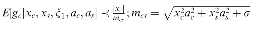
We say that center and surround are in the same normalization pool when they are co-assigned to a common mixer and deemed statistically dependent. This is the case, for instance, when the center and surround stimuli are statistically homogenous (see cartoon in Figure 1a, for patches that are within the zebra image). In this case, the Gaussian estimate is given by:
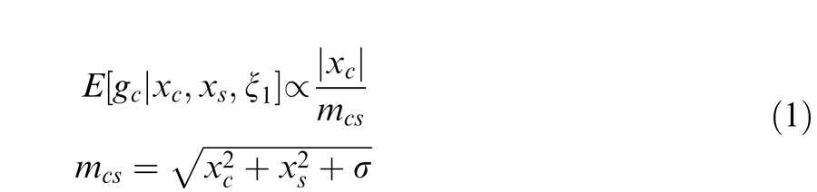 |
Here xc is the center unit activation and xs the surround unit (for readability, we assume just one filter in the center and one in the surround, although this can be extended to more filters); mcs is the gain signal that includes both center and surround and acts divisively (thus related to divisive normalization); σ is a small additive constant as typically assumed in divisive normalization modeling (Heeger, 1992; Schwartz & Simoncelli, 2001; Schwartz et al., 2009; here we fix it at 0.1 for all simulations); and ξ1 indicates inclusion of both center and surround in the normalization pool. The Appendix includes the full form of Equation 1, which contains a function f(mcs, n) to make the equation into a proper probability distribution. The function f(mcs, n) depends on both mcs and on the number of center and surround filters n. We have omitted the function f(mcs, n) in the main text for simplicity and to exemplify that this formulation is similar to the canonical divisive normalization equation (e.g., Heeger, 1992; see this point also in Schwartz et al., 2009; Wainwright & Simoncelli, 2000). However, note that in all simulations and plots in the paper, we compute the full form of the equation according to the Appendix. Also, the exact mixer prior changes the equation details but not the qualitative nature of the divisive normalization and the simulations (see Appendix).
More complex versions of the GSM can include a covariance matrix that departs from the identity matrix and is learned from natural scenes. This essentially modifies the gain signal in the denominator by allowing nonequal weighting for filters in the normalization pool. In most of the simulation examples presented here, as in Schwartz et al. (2009), we assume an identity covariance matrix. However, we also consider one neurophysiology example that includes different geometric arrangements of the inputs, with emphasis on collinearity (Wannig et al., 2011). For this, we apply an extended version of the model that relaxes the identity matrix covariance assumption, allowing surround filters in different locations to have different weights in the gain signal (Coen-Cagli et al., 2009). In this case, the gain signal is given by:
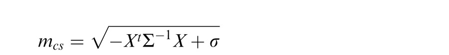 |
where Σ is the covariance matrix and X = (Xc, Xs).
Center and surround in different normalization pools
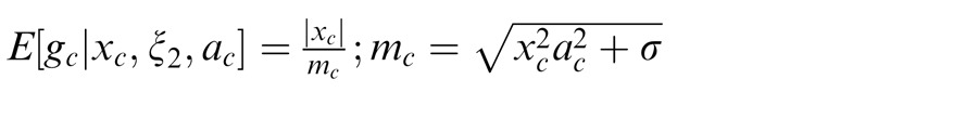
We have thus far described the condition in which the surround is in the normalization pool of the center. Similarly, we consider the case in which the surround is not in the normalization pool of the center, i.e., they are not co-assigned to a common mixer and are deemed independent. This is the case, for instance, when center and surround stimuli are inhomogeneous (see cartoon if Figure 1a, when center and surround patches are across the border of the zebra image). We solve for the Gaussian estimate, E(gc | xc, ξ2), where ξ2 indicates inclusion of only the center and not the surround normalization pool.
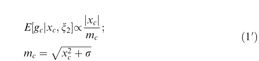 |
Here the divisive gain signal mc includes only the center filter responses.
Full model as a mixture of independent and dependent conditions
For any given input stimulus, the two Gaussian estimates (Equations 1 and 1′) are weighted by the posterior probability that the center and surround are in the same normalization pool for the given stimuli. The model output is therefore given by:
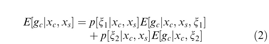 |
Equation 2 includes a first term in which the surround normalizes the center filter activation and thus is in its normalization pool (Equation 1) and a second term in which the surround does not normalize the center activation and thus is not in its normalization pool (Equation 1′). In addition, the strength of the normalization signal is dependent on the (posterior) weighting of the two terms in Equation 2, resulting in a generalized form of divisive normalization.
Here the priors for the two cases of surround normalizing the center or not are (p[ξ1], p[ξ2] = 1 − p[ξ1]). The posteriors for the surround normalizing the center or not given filter activations to an input stimulus are (p[ξ1 | xc, xs], p[ξ2 | xc, xs]). In this paper, we treat the priors as a free parameter and calculate the posterior assignments given an input stimulus similar to Coen-Cagli et al. (2012) using Bayes (see Appendix). Figure 2 shows how the posterior co-assignments vary as a function of orientation difference and contrast for different priors, intuitively related to the suggestion above that more homogenous center and surround stimuli are more likely to be in the same normalization pool. When the prior probability of co-assignment is set to 1, then the posterior probabilities become (p[ξ1 | xc, xs] = 1, p[ξ2 | xc, xs] = 0), which is essentially the canonical divisive normalization model in which the surround always normalizes the center for any input stimuli (Figure 1b).
Figure 2.

Influence of prior co-assignment parameter (i.e., probability over all stimuli that surround is in the normalization pool of the center) on estimated posterior co-assignments in the model (i.e., probability that surround is in the normalization pool of the center, given the observed center and surround stimuli). This is plotted as a function of (a) orientation difference between the center and surround, and (b) contrast of the center when the surround is set at maximum contrast.
Other model details
We follow Schwartz et al. (2009) in assuming that the normalization pool of the surround units has the same orientation preference as the center units. This is motivated from the observation that statistical dependencies are prominent for similar center and surround orientations (Coen-Cagli et al., 2012; Schwartz & Simoncelli, 2001). Therefore, when the surround normalizes the center target, this amounts to a tuned surround normalization (see also Chikkerur et al., 2010; and Ni, Ray, & Maunsell, 2012, regarding tuned surround normalization and in the middle temporal visual area [MT]). In addition, we assume that the linear front-end units in center and surround locations are given by idealized Gaussian tuning curves:
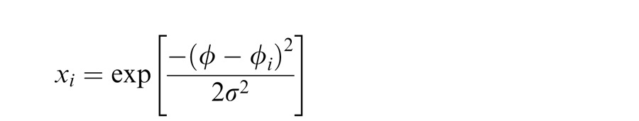 |
with i corresponding either to center or surround location, ϕ to the stimulus orientation, and ϕi to the preferred orientation of the neural unit.
For the perceptual tilt illusion simulations, we use a standard population vector read-out (Georgopoulos, Schwartz, & Kettner, 1986), identical to the approach in Schwartz et al. (2009). Specifically, we consider a population of center units, E( | xc, xs), with 360 preferred orientations. The estimated center angle given by:
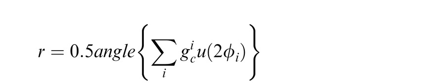 |
where ϕ is the preferred angle of unit i, u(ϕ) is a two dimensional unit vector pointing in the direction of ϕ, and the doubling takes account of the orientation circularity.
Cortical flexible normalization model with top-down attention
The generative model we described above specifies how to generate filter outputs corresponding to center and surround locations, and we assume that given these outputs, cortical neurons in a center location estimate the local Gaussian component via a generalized form of divisive normalization. We assume that in the face of attention, neurons continue to compute this local structure, since all the attention tasks we focus on are concerned with a local task in a central location in light of the contextual stimuli and indeed report the response of a neuron in the central location. We thus hypothesize that attention accentuates the attended filter outputs in the center and surround locations and that cortical neurons then compute the local estimate (i.e., Gaussian corresponding to the center location) as before. Attention to the surround only influences this computation when center and surround stimuli are inferred to be statistically dependent. The model therefore weights more the contribution of the attended locations, as if they are more believable or reliable, but only if the attended locations are considered dependent with the center location. In the Discussion section, we discuss the relation of our approach to functional models of attention.
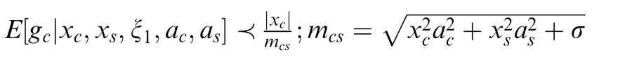
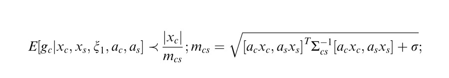
We first consider attention for the case that center and surround are co-assigned and in the same normalization pool. The outputs for center and surround are now given by: acxc and asxx, where ac and as are center and surround attention weights and xc and xs are the filter outputs without attention as before. The output of each spatial location may be multiplied by its own attention weight, but to simplify the notation, we show the equations for a single surround location and attention weight.
The observed output with attention is given by a GSM model with a common mixer multiplying a Gaussian: gcv = acxc; gsv = asxs. The model neuron estimates the Gaussian corresponding to the center unit, which depends on both acxc and asxs:
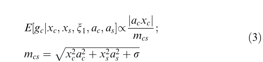 |
Here mcs is the gain signal with attention that includes both center and surround filter activations. The divisive signal weights more heavily the location that is more strongly attended. In addition, attention to the center location weights both the numerator and the divisive gain signal, while attention to the surround weights only the divisive signal.
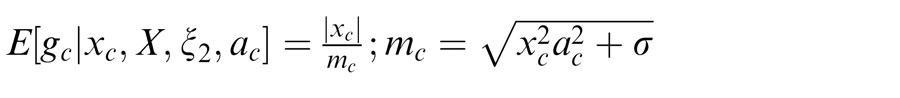
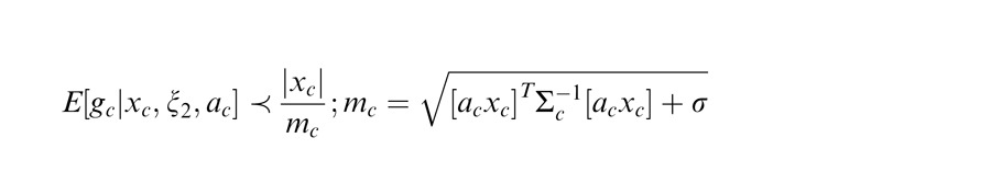
When the surround is not in the normalization pool of the center, then attention to the surround has no influence on the estimation. Attention to the center is given by:
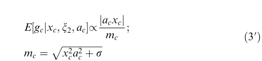 |
For attention weights set to 1, Equations 3 and 3′ reduce to Equation 1 and 1′ above.
As before, the full model is a weighted sum of Equations 3 and 3′, according to the probability of co-assignment given the input stimulus and the attentional parameters in center and surround:
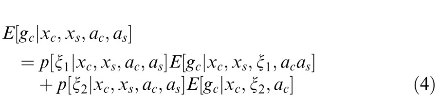 |
For Equation 4, we need to estimate the (posterior) probability of co-assignment given the input stimulus:
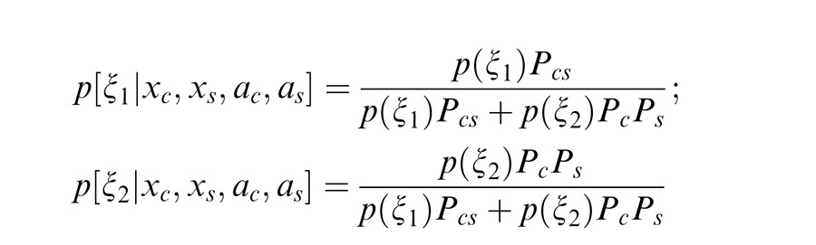 |
The term Pcs is the likelihood of the observed filter values under the assumption that center and surround are coordinated (ξ1). Similarly, PcPs is the likelihood under the assumption that center and surround are independent (ξ2). The equations for Pcs, Pc, and Ps are given in the Appendix and depend on the gain signals for center and surround mcs, center alone mc, and the surround alone ms, as well as the number of filters in the center and surround. Note that attention also influences these gains since it acts multiplicatively on the filter outputs, and so can also affect these co-assignment probabilities. Intuitively, when the gains of center and surround are more similar, they are more likely to be co-assigned.
In summary, the resulting form of attention influence in the model has two main features. First, it is similar to the proposal of Reynolds and Heeger (2009), in that attention can weight both the numerator and the divisive signal. But it is different in terms of the normalization pools that are part of the original statistical formulation. Attention alters how much we should weight the units in a given normalization pool that are contributing to the estimated model neuron response. For instance, if one attends to the surround location, then if center and surround are deemed generated with a common mixer, the surround signal is weighted more heavily, as if its contribution is accentuated due to the attention in this computation (and similarly, for attention to the center).
Second, attention also acts on the co-assignment probability and so can influence the composition of the normalization pool for given experimental stimuli, as a function of properties such as contrast, orientation, and geometric arrangement of the stimuli. In the Results section, we show a few neurophysiology examples in which we suggest that the composition of the normalization pool is critical. We also show that one can conceive of stimuli for which attending to the surround leads to competing effects such as (a) a heavier weight of the surround units (similarly to the case above), but at the same time (b) a lower probability that the center and surround are deemed dependent. This leads to nontrivial predictions that differ from Reynolds and Heeger (2009).
Model parameters and fits
In the model simulations, we fixed the additive constant in the model to 0.1, and the prior probability that surround is in the normalization pool of the center to 0.5 (from which we always infer the posterior probability using Bayes, given the particular experimental stimulus, as stated in the Methods section).
In one of the simulations (Figure 5), we optimized the parameters of the model to best match the Sundberg et al. (2009) data with a least-squares fit. We did this for both the canonical and flexible models. In the canonical fit, we also included an extra weighting factor for center and surround terms (that is fixed across all input stimuli) to allow for more flexibility: wcws such that mcs = . Both versions with and without this added (fixed) flexibility yielded similar results. We specifically fit the weighting factors, the additive constant, and the attend yes and no conditions: wc, ws, σ, ayes, and ano (the fits were 2.0294, 0.5395, 0.0891, 0.3148, and 0.2073). For surround attention, we set as = ayes and ac = ano; for center attention as = ano and ac = ayes; and for distant attention, as = ano and ac = ano. For the flexible normalization model we fit σ, ayes, ano, and ξ (the fits were 0.01, 0.354, 0.14, and 0.32), where the last term is the prior for assignment.
Figure 5.

 |
 |
In one of the simulations (Figure 6), we included the covariance matrix learned in Coen-Cagli et al. (2009), which relaxed the assumption that the denominator weighted equally each surround filter. Specifically, the inverse covariance was such that for the assigned condition both the variance for the collinear location and the covariance between the collinear and center location were higher.
Figure 6.

Flexible versus canonical models for geometry. (a) Simulations of Wannig et al. (2011) attention data. Cartoons show the stimuli and location of attention. Both the flexible and canonical models capture the larger facilitation for collinear attention in the Wannig et al. (2011) data. (b) Simulations without attention based on Cavanaugh et al. (2002), with cartoons and simulations adjusted to match the Wannig et al. (2011) setup. Only the flexible model captures the greater suppression for collinear than diagonally placed stimuli. Attention weights are set to 2 and 1, respectively, and the additive constant to 0.1. The flexible and canonical models are as in Figure 5, but include a nondiagonal inverse covariance matrix capturing the geometry:
 |
 |
Results
Model behavior
We first demonstrate some of the main properties of the model, by varying the attention weights of either center or surround, and examining the result as a function of whether center and surround are in the same normalization pool. We show the two extremes of either the surround not in the normalization pool of the center (co-assignment probability 0), or surround in the normalization pool of the center (co-assignment probability 1). All other values of Equations 3 and 3′ are held fixed, and the center and surround unit (linear) activations are set to a value of 1. In each condition, we depict the estimated Gaussian of a given center unit (i.e., the estimated output of the center unit, according to the model).
Figure 3a depicts the condition in which center and surround are not in the same normalization pool, i.e., do not share a common mixer in the model. In this case (Equation 3′), increasing the surround attention when the center weight is held fixed at 1 has no effect on the estimated model output. In contrast, increasing the center attention weight when the surround weight is held fixed at 1 increases the estimated output. In Figure 3b, the center and surround are assumed in the same normalization pool, i.e., they share a common mixer in the model and are co-assigned. In this case, increasing the center attention weight (blue line, with the surround attention weight fixed at 1) still increases the estimated response. In addition, increasing the surround attention weight now decreases the estimate (black line, with the center attention weight fixed at 1). This is due to Equation 3, in which the surround unit outputs affect the response of the center unit via the divisive normalization signal. Note also that for high probability of co-assignment, the estimated response increases more rapidly for large values of center attention (compare the blue lines in Figure 3a and b for center attention weight above 1).
Figure 3.

Model behavior for different parameter changes. (a) Model response (i.e., Gaussian estimate in the GSM model; see main text) when surround is not assigned. In the simulation, we either vary the surround attention weight when the center attention is fixed to 1 (black line), or we vary the center attention weight when the surround attention is fixed to 1 (blue line). Additive constant is set to 0.1 and number of filters set to 4 (one center filter and three surround filters; n = 4). Note that if we change the number of surround filters, the result remains the same since the surround is not assigned. (b) Same but when surround is assigned to normalization pool of center with probability 1. Cyan and gray lines correspond to n = 2, 3, 5, and 6, resulting in similar qualitative effect.
We next discuss this form of model in relation to experimental data. Cortical neurons are strongly influenced by surround stimuli. We specifically examine data in which surround effects in cortex (such as the amount of suppression or facilitation, or changes in contrast response curves) are influenced by attention. We start by showing that the model can replicate key experiments explained by divisive normalization, as well as simple extensions that require a tuned surround normalization pool. We then go on to model physiological data that we suggest is well suited to our form of flexible normalization pools. Finally, we propose new experiments targeted at providing a better test case for distinguishing the models.
Neurophysiology simulations: Canonical and tuned divisive normalization
We first show that our model replicates some key attention results that have previously been addressed due to the similar form of attention modulation as in Reynolds and Heeger (2009). The model can capture data in which the size of the attention field is critical for changes in contrast response functions: namely, capturing both so-called contrast gain and response gain, which have been observed in the experimental literature. In Figure 4a, we include a small optimally oriented stimulus within the center receptive field (RF) and a large attention field (i.e., attention to both center and surround units). Attention causes a leftward shift in the contrast response function (i.e., contrast gain) relative to the nonattended condition. Figure 4b depicts a larger stimulus covering both the center and surround unit locations and a smaller attention field within the center unit RF. Now, attention results in an upward shift of the contrast response function (i.e., response gain). In the simulations, center and surround are in the same normalization pool, since the input stimuli have similar orientation. The behavior in the model arises due to the nature of Equation 3, which has similar properties to the Reynolds and Heeger (2009) model, with attention to the center weighting both the numerator and denominator and attention to the surround weighting only the denominator. Note, however, that this behavior is only fully observed if the contrast response function is saturating, which in our formulation depends on the mixer prior and indeed holds for the prior we have chosen (see Appendix).
Figure 4.

Contrast versus response gain in the model (after Reynolds & Heeger, 2009). (a) Stimulus confined to center of RF, and attention field (red filled circle) includes center and surround locations; (b) stimulus extent includes center and surround locations, while attention field is confined to the center location. In both panels, attended location weight set to 3 and unattended to 1, and number of filters is set to 2 (n = 2). The qualitative result does not depend on the number of filters.
Our model also replicates another key result (not shown) of changes in orientation tuning due to attention (McAdams & Maunsell, 1999). The attention is either to an oriented stimulus (“attend center” condition) or to a color blob, which constitutes the contextual stimulus (“attend away” condition). Attention to the center scales the height of the tuning curve multiplicatively, both in the V4 data and model. In the model, this is due to the increase in the estimated response for larger center attention (Figure 3), behaving similar to the Reynolds and Heeger model (2009). Similar multiplicative scaling has been noted in area V1 (McAdams & Reid, 2005).
Our model also accounts for data that require tuned surround normalization with attention, an aspect that is unconstrained in descriptive normalization models, but that has been suggested in other recent modeling approaches (Chikerrur et al., 2010). By assuming that surround suppression in V4 is also orientation tuned as in V1 (see discussion in Sundberg et al., 2009, and their reference to Schein & Desimone, 1990), then we expect to see experimental differences in attention to the surround for parallel versus orthogonal surround. In particular, when the surround stimulus orientation is orthogonal to the center stimulus, then we predict no effect of attending to versus ignoring the surround. This prediction also comes about in a canonical divisive normalization model that includes a tuned surround (e.g., by setting the co-assignment probability of surround in the normalization pool of the center to 1 in our model). In contrast, a model that includes an untuned surround, and thus allows all surround orientations to contribute to the normalization signal, would result in surround suppression for the attend surround condition. Although the different conditions have not been tested extensively or systematically, some neurophysiology data indeed suggest that there is no effect of attention in V4 when the surround is an orthogonal orientation to the center (Moran & Desimone, 1985).
Neurophysiology simulations: Flexible normalization pools
We are particularly interested in data for which our model diverges from the canonical divisive normalization model. It should be noted that experimental data thus far are scarce. However, we suggest that recent data are compatible with our proposal. We also simulate model predictions that are more targeted at testing the flexible normalization model.
Surround suppression as a function of contrast and attention
We first consider recent data showing a strong effect of attention to the surround when the surround is the same orientation as the center in V4 (e.g., Sundberg et al., 2009). Sundberg et al. (2009) measured attention in V4 neurons for iso-oriented stimuli in the center and surround, including a control of attending to a distant surround. One main result in the data is more suppression when attending to the surround and less suppression when attending the center: As Sundberg et al. (2009) point out, this is expected from a divisive normalization model of attention (Reynolds & Heeger, 2009). In addition to this observation, we focus on a particular aspect of the Sundberg et al.'s (2009) data that we show is of interest from the point of view of the flexible model, namely the modulation with attention as a function of stimulus contrast. The main idea in the flexible model is that the contrasts of the center and surround stimuli, and the attention condition, affect the posterior probability of assignment and therefore influence the amount of surround suppression. We go through the thought process and simulations in more detail below, showing that the flexible model, but not the canonical model, can capture a particular trend of contrast dependence of surround modulation in the data.
To quantify the surround modulation, Sundberg et al. (2009) calculated the surround modulation index (SMI) for attending to a given center (SMI_center), surround (SMI_surround), or distant location (SMI_distant). The SMI index pertains to the response of a neuron with attention to the given location (center, surround, or distant) when the surround stimulus is present versus attention to the same location when there is no surround stimulus:
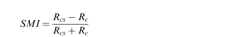 |
As can be seen in Figure 5a, both the canonical and flexible normalization models can capture a main trend in the data of more surround suppression when attending to the surround than when attending to the center and of more intermediate suppression when attending to a distant location. Also, as reported in Sundberg et al. (2009), for both models the SMI index is stronger (more negative) when the center stimulus contrast is low than when it is high contrast. Note that the surround stimulus is fixed to a high contrast in these experiments, while the center stimulus contrast is varied. In both models, the surround attention weights the surround filter activation more heavily, leading to more suppression, and the distant attention constitutes a control in which center and surround filter activations are weighted equally (i.e., both are not attended).
In addition, when the data is replotted (Figure 5b, left), it is also evident that for low center contrast, the SMI index for attending to surround or distant locations are more similar; as the center contrast increases, the SMI index for surround and distant locations are more different. We next show that a canonical divisive normalization model could not account for this trend (Figure 5a, b, middle column) and that it is better captured by the flexible model (Figure 5a, b, right column).
In the canonical model, for low center contrast, the difference between the surround and distant attention is instead more pronounced in the canonical model. This can be seen in the canonical model from the term:
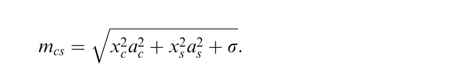 |
For low center contrast, the center filter activation is low, and so the surround activation term (weighted by the attention signal) becomes more prominent. For high center contrast, this difference is diminished in the canonical model (it can flatten if the additive constant is very large or if the center filter activation is not in the denominator due to a zero weighting factor, but it cannot reverse the trend). To demonstrate this, we show the resulting simulation in Figure 5b (middle) by fitting the parameters of the canonical model (see Methods) to best match the SMI data in 5a (left). The full data fits are shown in Figure 5a (middle). The difference between the attend surround and distant conditions are shown in Figure 5b (middle). We tried fitting several versions of canonical model (see caption of Figure 5 for including large divisive weight) and manually exploring the parameter range, and could not reverse the trend to match the data.
We then considered the flexible normalization model and found that it could capture this trend of modulation index as a function of contrast in the Sundberg et al. (2009) data (Figure 5a, b, right). In the flexible model, this was due to the posterior assignment weights (Figure 5c, right), which in turn control the amount of surround suppression. The strength of surround modulation for the surround attention condition increases more rapidly as the center and surround stimulus contrasts are more similar (therefore, as the center contrast is increased; see cartoon in Figure 5).
Surround geometry and attention
The data of Wannig et al. (2011) suggest that attention effects depend on the geometric arrangement of stimuli in the surround. Using stimuli that comprise several oriented bars, they found, for instance, that when center and surround bars are matched in orientation, then attention to a collinear surround leads to more facilitation than attention to a diagonally placed surround (see stimulus cartoon in Figure 6).
To address the Wannig et al. (2011) data, we considered the flexible attention model with a covariance matrix that is matched to those learned in Coen-Cagli et al. (2009), such that the covariance is higher between collinear filters when center and surround are co-assigned. In the experiments, the stimulus arrangement always included both parallel and diagonal surround bars, and attention was manipulated. In this case, the estimated co-assignment probability in the model remained high for both attention conditions (Figure 6a, right). The response of the flexible model was therefore dominated by the covariance weights in the denominator, leading to less surround suppression in the collinear attention than the diagonal attention case (Figure 6a, middle). We note that a canonical divisive model that is handed the same covariance matrices learned in Coen-Cagli et al. (2009) could also capture this result (Figure 6a, left), following a similar argument. Since the estimated assignment probability in the flexible model is near 1, the two models behave similarly in this case. As in Wannig et al. (2011), this effect was not present when the stimuli at the two locations were orthogonal (simulation not shown).
However, there are also data on surround suppression and stimulus geometry, in the absence of attention. We treated such data as a control condition, which the model should also be tested against. In particular, Cavanaugh, Bair, and Movshon (2002) found that when center and surround grating orientations are similar, there is more surround suppression when the surround stimulus is arranged collinearly. The flexible model can address this result, as we have also shown previously (Figure 6b, middle; see also Coen-Cagli et al., 2012, for a more complete simulation of the Cavanaugh et al., 2002 geometry data). Note that in this experiment, the stimulus configuration does change for the different experimental conditions, and the surround is either arranged collinearly, diagonally, or parallel with the center. In the flexible normalization model, the estimated co-assignment weights are significantly higher for the collinear than the diagonal or parallel stimulus arrangements (Figure 6b, right; since collinear stimuli are deemed as more assigned in the model inference, due to the learned covariance weights). As a result, for the collinear stimuli, higher co-assignment brings about more surround suppression in the flexible model, consistent with the data. This is crucially different from the Wannig et al. (2011) stimulus configurations, in which the collinear stimuli were always present in both conditions, which led to a large co-assignment in the model for all stimulus conditions.
We can again ask whether a canonical normalization model can explain the results of Cavanaugh et al. (2002). As before, we consider a canonical model with the same covariance matrix and set the co-assignment weights to 1. In this case, the canonical model cannot account for the Cavanaugh et al. (2002) data (Figure 6b, left). With the weights set to 1, the canonical model instead produces less suppression for the collinear than other stimulus arrangements. It is of course possible instead to hand-design the weights of a canonical divisive model differently so that they are compatible with the Cavanaugh et al. (2002) result. However, the same canonical model would then fail to account for the Wannig et al. (2011) data. That is, one cannot hand-design a set of weights in the canonical model that would account for both sets of data simultaneously. We assume here that the effects in the Wannig et al. (2011) data are due to the nonclassical receptive field, i.e., that the surround bars are indeed outside the classical RF, although we cannot rule out that there are also influences of the bars impinging on the classical RF. In summary, the flexible model therefore suggests a means of addressing two disparate sets of geometry data, with and without attention. Since the experiments were each run separately with different conditions, there is room for further testing with neurophysiology in which the geometric stimulus configurations and attention manipulations are recorded in the same neuron.
Model predictions
As noted earlier, existing neurophysiology data are fairly sparse in terms of testing the kind of issues that are critical for the flexible normalization model. However, the goal of building models such as ours is not only to show compatibility with some existing data, but crucially, to make new predictions for experiments that have not been done and are motivated by the theory.
In our model, the co-assignment probabilities for a given input stimulus are affected by attention. One can conceive of experiments for which these would be critical and for which our model predictions would be expected to depart from other divisive models of attention. Of particular interest are cases in which the center stimulus is nonoptimal for the neuron and the surround stimulus is optimal. As a consequence, surround attention increases the surround gain but decreases the co-assignment probability (because center and surround influences are now even more different and less likely to be co-assigned). This can result in attention to the surround, reducing surround suppression, rather than enhancing it as would be predicted in divisive normalization models that do not include flexible normalization pools. This can be contrasted with the case of an optimal center and non optimal surround, in which case attention to the surround increases both the surround gain and the co-assignment probability (because it makes center and surround responses more similar), leading to more suppression.
Figure 7 depicts the model predictions contrasting the flexible and canonical model (assuming a tuned surround in both). We vary the distance between the center and surround orientations, with the center either optimal or nonoptimal. To simulate the canonical model, we used a reduced version of our model without normalization pools (i.e., probability of surround co-assigned to center normalization pool always set to 1). The two models behave similarly for optimal center and varying the surround; in both, the amount of modulation by attention depends on the difference between the orientations of center surround. However, the canonical model predicts that for a nonoptimal center stimulus and optimal surround, the modulation by attention is essentially similar and strong, regardless of the center stimulus orientation (Figure 7a). The flexible model, in contrast, predicts that the amount of attentional modulation depends on the difference between the orientation of the nonoptimal center and optimal surround (Figure 7b). This is, in turn, a consequence of the co-assignment probabilities (Figure 7c). This example points to the suggestion that attention may have similar effect as contrast (Coen-Cagli et al., 2012) in terms of grouping of center and surround, which results in some nontrivial predictions that have yet to be tested experimentally.
Figure 7.

 |
 |
Discussion
We have focused on contextual effects and attention within a generative class of scene statistics model. We have previously linked our modeling approach to a generalized form of divisive normalization model that is sensitive to the statistical homogeneity of the input and includes a flexible divisive normalization pool (Coen-Cagli et al., 2012; Schwartz et al., 2009). Here we have added attention to this class of model, via weighting more heavily the contribution of the center and surround units that are attended and in the same normalization pool. We have shown that the resulting attention model can explain some cortical data pertaining to spatial contextual influences of orientation and attention. In particular, our model replicates some neurophysiology results that have been previously modeled with divisive normalization (Figure 4). Our model also addresses some additional neurophysiology spatial context data (Figures 5 and 6) and, importantly, makes new testable predictions (Figure 7), given the extension to stimulus-dependent normalization pools.
We next describe the relation to divisive normalization models in more detail, as well as functional models of attention and the implications of our model from a functional standpoint. We then discuss the implications of our model for neurophysiology and for perception, and extensions of the modeling.
Relation to and extension of divisive normalization models of attention
Our model relates to divisive normalization formulations of attention (Reynolds & Heeger, 2009; see also Ghose, 2009; Lee & Maunsell, 2009) and particularly to the divisive normalization model described by Reynolds and Heeger (2009). Reynolds and Heeger (2009) are more permissive in the divisive normalization pool and do not have a computational method to set the surround selectivity in the divisive pool. They assume that the normalization pool is fixed rather than stimulus dependent.
Recent scene statistics approaches (e.g., Coen-Cagli et al., 2012; Schwartz et al., 2009) suggest that surround effects depend on properties such as the relative orientation and contrast, which influence whether units are in the same normalization pool. Here we propose that attention could be manipulated within this extended form of model. The form of cortical model is thus motivated from scene statistics, potentially providing an extra layer of functional interpretation. We have shown that some existing experimental data on attention are compatible with the suggestion of stimulus-dependent normalization pools (e.g., Figures 5 and 6), although we note that the existing data on this topic is sparse (see subsection on experimental implications).
Our model extends previous divisive normalization models by incorporating co-assignment probabilities that can be modified not only by the sensory input (such as contrast and orientation) but also by attention; this in turn influences the normalization pools. Indeed, an additional proposal of the statistical model is that attention could actually influence the (posterior) probability that center and surround are deemed dependent. We suggest that a rational may be seen in the analogy of contrast and attention effects within the model. The judgment about the dependence between a single pair of adjacent regions is necessarily a probabilistic one: The model can only compute a probability that the given regions are an instance of a dependent (or independent) process. Changes in contrast (and attention) can change the evidence in favor of one hypothesis or the other. As for contrast (Coen-Cagli et al., 2012), we suggest that the intermediate cases in which there is some probability that center and surround are dependent (but it is not extremely near 0 or 1) are most interesting and may be biased by attention. For instance, if attention to the surround makes the center and surround appear even more different, then the surround suppression could be reduced according to the model. We have shown a concrete predictive example (Figure 7).
We note that there are various forms of attention in the literature, including: spatial, feature, and surface or object-based attention. For spatial attention, we suggest that the question of whether the spatial context is in the divisive normalization pool of the target is critical. For feature attention to the opposite hemifield, the contextual stimulus is too far away spatially and exerts no divisive influence, neither in the flexible model nor in Reynolds and Heeger (2009). In this case, we assume that the attention influence itself follows the suggestion of Reynolds and Heeger (2009), and the flexible and canonical models do not diverge. If there is an interaction of both feature and spatial attention (e.g., one is cued to a feature in the nonclassical surround), then the models could, however, diverge due to the potential for divisive normalization. Perceptual grouping of surfaces or objects (where the grouping extends to spatial regions outside the classical receptive field) are interesting from the point of view of the flexible model. We have specifically considered the geometric grouping of orientation, as in Wannig et al. (2011). We have shown that the flexible model is sensitive to collinear versus other geometrical configurations, thus diverging from the canonical model (Figure 6). These directions might be expected to generalize to other feature configurations beyond the scope of this model: For instance, in area MT, Wannig, Rodríguez, and Freiwald (2007), suggest that when there are two spatially overlapping surfaces, then attention to a feature in one surface essentially “spreads” across the surface. Other perceptual studies (e.g., Festman & Braun, 2012) have shown attention spread when the attended and ignored fields conform to a complex perceptually grouped motion.
Our model is not tied to a specific mechanistic implementation, although there are a range of mechanistic models for divisive normalization (see, e.g., references in Schwartz, Hsu, & Dayan, 2007; Carandini & Heeger, 2012, reviews), for attention (see, e.g., references in Reynolds & Heeger, 2009; Baluch & Itti, 2011, reviews; Mishra, Fellous, & Sejnowski, 2006; Tiesinga, Fellous, Salinas, José, & Sejnowski, 2004); as well as the intersection of the two (e.g., Ayaz & Chance, 2009). The co-assignments in our model might be related to network states switching between regimes in which the surround is active or inactive or to interneuron's pooling different subpopulation outputs (Salinas, 2003; Schwabe, Obermayer, Angelucci, & Bressloff, 2006; see Coen-Cagli et al., 2012 and related references).
Functional models of attention and functional implications of our approach
The functional goal of attention is a topic of great interest and has been addressed in other computational modeling approaches. Dayan and Zemel (1999) modeled attention as increased certainty (given tradeoff between accuracy and metabolic cost) in a population of cortical neurons for coding a stimulus property such as orientation. A number of computational models of attention have focused on Bayesian modeling frameworks, given uncertain sensory inputs and top-down attention priors (e.g., Chikkerur et al., 2010; Rao, 2005; Yu & Dayan, 2005). Other recent work has suggested that scenes are too complex to allow exact Bayesian inference and that attention might serve to improve and refine the approximations (Whiteley, 2008).
Yu and Dayan (2005) considered optimal inference in the face of (e.g., spatial) uncertainty and have shown that this can address various issues and classes of perceptual attention data not addressed within our framework, such as the Eriksen task and load (e.g., Dayan, 2009; Dayan & Solomon, 2010; Yu et al., 2009). Chikkerur et al. (2010) assumed that the system should infer the identity and position of the visual input and showed that their resulting form of model is equivalent to Reynolds and Heeger (2009). In their model, attention essentially increases the prior probability of a particular feature or location and, via Bayes, is incorporated both in the numerator and the denominator of the formulation. Their model amounts to a tuned surround normalization, but does not address normalization pools. Chalk, Murray, and Series (in revisions) explained modification of the prior as a strategy to optimize the expected reward in detection tasks, under the hypothesis that the brain learns a probabilistic model of both stimulus statistics and reward statistics. These studies thus suggest a normative framework for the type of attentional modulation that we have assumed. Here, we focus instead on its interactions with scene statistics.
The attention model of Spratling (2008) does adopt a scene statistics approach, but within a predictive coding framework (e.g., Rao & Ballard, 1999, modified to be multiplicative). Their model results in divisive normalization due to the modified nonlinearity from the original predictive coding. Attention multiplicatively modulates the model neurons and essentially biases the attended neurons to win in the competition over other neurons and to suppress nonattended neurons. Although their approach is described quite differently from ours, the divisive normalization is driven by this competition and proposed to facilitate binding, which also goes beyond more canonical divisive normalization frameworks with a fixed normalization signal. However, they do not focus on issues of the heterogeneity in scenes and normalization pools, which is the main focus here.
We suggest that attending to a location in the surround influences the center computation only when they are inferred to be statistically homogenous or more generally part of the same texture or extended object. There are at least two ways of interpreting our model suggestion in this vein. First and perhaps more intuitively, attention may be thought of as enhancing the apparent contrast of the visual input at a given location, as has been suggested before (e.g., Carrasco, Ling, & Read, 2004; Carrasco, 2011, and references therein). If one attends to the surround, then the assumption that the surround appearance is enhanced leads to the proper adjustment in the local estimation of the center when center and surround are considered statistically dependent; conversely, when center and surround are independent, the enhanced contrast of the surround has no effect on the estimation.
A second related way to consider the effect of attention is that the visual input in the attended location may become a more reliable cue than the unattended location, therefore weighting its contribution more heavily in the estimation of the center, but only if they are considered dependent. As an analogy, consider the case of lightness perception (Adelson, 2000). The luminance is a more global shared property, and the reflectance is a more local property. If one aims to estimate a local reflectance in a given position, then if attention is to a surround location sharing the same luminance, the surround might be more heavily weighted in such computation as if that information is more enhanced or more reliable. In contrast, attending to a location that is known to have an entirely different luminance would not affect the local estimation. This suggests that attention could serve to improve local estimates by properly setting the normalization pools. This concept could be formalized by adding an explicit noise term to the model and evaluating the local estimation in a task. This direction offers a route for future work but is beyond the scope of this paper. In addition, we suggest that attention could change the probability that center and surround are considered to be part of the same global object in this estimation.
Neurophysiological implications
We have modeled a range of attention neurophysiology data in the literature, with emphasis on the interaction between surround modulation and attention. We suggest a number of directions for future experiments in neurophysiology to further test the model.
While there have been recent biological data on surround and attention, we still lack understanding of many issues, which are crucial for constraining and testing the modeling. For V4, we do not have good understanding of surround selectivity even without attention, although Schein and Desimone (1990) suggest that suppression in V4 outside the classical receptive field is stronger for preferred orientation. In contrast, while a lot is known about surround effects in V1 and its selectivity to properties of the stimulus such as the orientation, we know less about the interaction between attention and surround in V1. Some data point to attention effects in V1 (Chen et al., 2008; Roberts, Delicato, Herrero, Gieselmann, & Thiele, 2007; Roelfsema, Lamme, & Spekreijse, 1998) and to similarities in attention between V1 and V4 (e.g., McAdams & Reid, 2005; Motter, 1993).
In general, it would be desirable to have more systematic testing of surround tuning (e.g., for different orientations outside the classical receptive field) and attention manipulation in the same experiment. Most studies of attention either fix the surround orientation or do not control for it. The finding of strong effects for the fixed condition of an optimal surround (Chen et al., 2008; Roberts et al., 2007; Sundberg et al., 2009) and that the amount of attentional influence depends on the amount of surround suppression (Sundberg et al., 2009) are consistent with our model. However, more fine and systematic manipulations of optimal and nonoptimal orientations in the center and surround, with and without attention (e.g., Figure 7), would be a stronger test case. Indeed, it was the fine manipulations without attention for V1 that allowed us to test the generalized divisive normalization model more closely in the co-assignment regimes where it makes nontrivial predictions (Coen-Cagli et al., 2012); such systematic testing with attention would allow us to similarly constrain the attentional modeling.
We also briefly note other related neurophysiology work on attention, which is not particular to our model versus other divisive normalization approaches. Other work on surround neurophysiology (Chen et al., 2008) pertains to task difficulty in area V1. They report results from two classes of neurons: “regular-spiking” neurons and “fast-spiking” putative interneurons. We expect the regular-spiking neural data to be most compatible with our model. When we assume that the attention weight is stronger for the hard task than for the easy task, we can obtain the right qualitative flavor of these “difficulty-suppressed neurons” in simulation; that is, responses are more suppressed when attending to the surround (due to increased suppression in the denominator of the divisive normalization; not shown). However, our model in its current form (and indeed also related divisive models) does not include a distinct separation of difficulty-suppressed and difficulty-enhanced neurons, as suggested in the data. Other V1 work (Roberts et al., 2007) has reported differences in area summation curves due to attention, in which attention to the RF in the near fovea reduces the RF radius, and attention to the RF in the parafovea increases the RF radius or peak of the area summation curve. Although we do not have control of fovea and periphery in the model, it is possible that some of the changes may be due to the attention size relative to the RF size of the neuron (in an analogous suggestion to issues leading to response versus contrast gain in Herrmann, Montaser-Kouhsari, Carrasco, & Heeger, 2010; Reynolds & Heeger, 2009; our Figure 4). In the experiments of Roberts et al. (2007), the portion of the bar stimulus that required attention was a small luminance patch. To model the near fovea, one might assume that the attention field covers both center and surround units, since the RF is small and even a little jitter is likely to include the surround. Attention would then include more surround suppression and reduce the RF radius. To model the more peripheral RFs, one might assume that attention is confined within the center unit RF, because the attended region of the bar is small, and the RF is larger. Attention would then modulate only the center unit RF and not invoke more surround suppression. This argument is not special to our divisive normalization formulation and would be expected to hold for other related models.
Perceptual implications
In previous work, we have used a similar form of divisive normalization model to address the perceptual tilt illusion via a standard population readout (Schwartz et al., 2009). The attention model could also be used to tie in with such perceptual biases, but more understanding is needed regarding manipulating attention to center and surround in the tilt illusion.
In repulsive biases, which are apparent, for instance, in the classical tilt illusion for surround stimuli, the center orientation is perceived as tilted away from the surround more than it actually is. Such repulsive effects occur for small orientation differences between the center and surround stimuli. Such effects without attention can be explained by canonical divisive normalization (Schwartz et al., 2009). Surround stimuli can also induce weaker attractive effects for large orientation differences between the center and surround, an effect that arises in our model without attention from flexible normalization pools (Schwartz et al., 2009).
There has been work on repulsive biases in the face of attention with either other features or in the temporal domain (e.g., Liu, Larsson, & Carrasco, 2007; Prinzmetal, Nwachuku, & Bodanski, 1997; Spivey & Spirn, 2000; Tsal, Shaley, Zakay, & Lubow, 1994; Tzvetanov, Womelsdorf, Niebergall, & Treue, 2006). However, there is little data on tilt illusion and attention addressing these issues (although see work on spatial crowding and attention; Mareschal, Morgan, & Solomon, 2010). There are at least two different sets of studies suggestive of the main change in repulsive bias that could emerge from a canonical divisive normalization model. First, there have been studies on the temporal analog of the tilt illusion (Clifford, Wenderoth, & Spehar, 2000; Schwartz et al., 2007), namely on the tilt aftereffect, showing that attention to the temporal context can increase repulsive biases (Liu et al., 2007; Spivey & Spirn, 2000). Second, there have been studies on the motion direction analog of the tilt illusion (Clifford, 2002), namely the influence of attention on surround motion repulsion (Tzvetanov et al., 2006). This study reveals an increased bias when attending to the context and also hints at the possibility that attention to a target in the absence of attention to a context may lead to less bias.
We have found in our model that similar predictions hold for repulsive effects in the tilt illusion (Figure 8). For the simulations, we follow an experimental design inspired by Tsvetanov et al. (2006), but in the tilt domain. Specifically, we include a vertical center orientation and two possible surround orientations (at ±20°; this is also similar to the tilt aftereffect attention experiments), and manipulate attention in this setup. Attention to the center decreases the repulsive bias due to less suppressive weight from the surround context, and conversely, attention to the surround stimulus increases the repulsive bias further due to more suppression from the surround via the increased attention weight. This is more pronounced when there is only one surround orientation. This prediction would qualitatively hold also for the canonical divisive normalization model and does not require flexible normalization pools.
Figure 8.

Model prediction for tilt illusion and attention. Experimental design after Tsvetanov et al. (2006), but in the tilt rather than motion domain. Cartoons indicate the orientation of the surround context and center target stimuli. The surround stimulus is at −20° and/or +20°. Red circle indicates attention. For the tilt illusion bias, we plot the difference between the actual (0°) and perceived orientation. We include the following stimulus conditions, as in the cartoons on the x-axis: Attention to center with no surround stimuli; attention to the center in the presence of a surround tilted at −20; Attention to the center in the presence of +20 and −20 surround stimuli; attention to center and the −20 surround in the presence of +20 and −20 surround; attention to the center and +20 surround in the presence of only this surround. Note that the first and third conditions result in no tilt illusion (exactly 0°), since there is either no surround, or balanced surround influence, and the model includes no noise. The attention weights were set to 1 for the attended and 0.4 for the unattended. The cartoon only shows two surround stimuli for readability, but we assume as in the tilt illusion, a larger surround (here n = 5).
In addition, the main focus of previous psychophysical work has been with respect to repulsive biases and attention. An open question is whether attractive biases that occur for large (e.g., orientation or motion) differences between target and context stimuli can be modulated via attention. Although attractive biases are more elusive in perceptual data, this could constitute an interesting test case for our model. Attractive biases occur in the realm of lower (but not zero) probability of co-assignment in the flexible model (Schwartz et al., 2009), and attention could alter these probabilities and thus shift the angle that leads to maximal attraction. We have focused here on the perceptual tilt illusion and attention. Perceptual studies have also shown that attention can modulate the integration of target and collinear flankers (Freeman, Driver, Sagi, & Zhaoping, 2003). There are also more general interesting questions beyond attention to a single feature regarding how our perception of grouping and segmentation of textures, surfaces, and objects in the world interact with attentional processes.
Model extensions
There are also a number of directions to extend the modeling. We have assumed that an attention signal is known (as is often analogous to the way attention experiments are done); however, one can consider extensions to the scene statistics approach in which attention provides some form of supervision in the learning (for a recent review, see Baluch & Itti, 2011; and for a reinforcement learning framework, Chalk, Murray, & Series, personal communication and submitted; and for eye movements, see Hayhoe & Ballard, 2005). We have also not addressed the possibility of correlated variability between model neurons in our population, an aspect that has received recent emphasis in the attention literature (e.g., Cohen & Maunsell, 2009, 2011; Mitchell, Sundberg, & Reynolds, 2009). An important question for the future is whether the flexible normalization extends to other grouping aspects, such as occlusion and figure-ground. Indeed, such issues are expected to influence whether the surround is in the normalization pool of the center. We have assumed that higher cortical areas hierarchically inherit the orientation selectivity of earlier visual areas. To address attention effects that are more specific to midlevel vision, we expect that the model would need to be expanded hierarchically to learn more complex features beyond orientation.
More generally, spatial context and temporal context (e.g., adaptation) are closely tied (Schwartz et al., 2007), and there are indeed tilt aftereffect data that could be explained by assuming a similar form of model in time as in space. The relation between neural adaptation and attention is poorly understood physiologically. There is great interest in obtaining a more unified understanding of the interaction between the signal statistics in space and time, and attention factors.
Acknowledgments
We are very grateful to Peter Dayan and Adam Kohn for helpful discussions and comments on the manuscript, and to Mathew Chalk and Peggy Series for comments on the manuscript. This work was funded by the NIH grant CRCNS-EY021371, and the Alfred P. Sloan Foundation (OS).
Commercial relationships: none.
Corresponding author: Odelia Schwartz.
Email: odelia.schwartz@einstein.yu.edu.
Address: Dominick Purpura Department of Neuroscience and Department of Systems and Computational Biology, Albert Einstein College of Medicine, Bronx, NY, USA.
Appendix
Gaussian estimate
As in previous work on the Gaussian Scale Mixture (GSM), the generative model is only well defined with a prior set on each of its components. The Gaussian component by definition includes a Gaussian prior as discussed in the main text, and for the mixer variable v, we assume a loglogistic prior. The exact form of the Gaussian estimate in the GSM depends on the mixer variable prior (see also Wainwright, Simoncelli, & Willsky, 2001). This does not affect the divisive form and qualitative nature of the simulations reported here, but influences the exponent of the numerator and denominator and therefore the saturation of the contrast response function. Here we use a loglogistic prior, which leads to a saturating curve. In previous modeling we have used a Rayleigh prior (Coen-Cagli et al., 2012; Schwartz et al., 2009), for which the exponent of the denominator is smaller; this can accommodate all the results reported here except for the needed saturation of the contrast response function for obtaining the results of Figure 4 on changes in contrast versus response gain with attention. Different neurons have different saturations, and from our perspective here (as in other divisive normalization formulations), we assume saturation via this choice of mixer prior.
Without loss of generality, we write out the case of center and surround co-assigned and therefore sharing a common mixer. We also write out the equations without attention for readability. Incorporating attention would (as described in detail in the main text) change xc to acxc and xx to asxs in all the equations below.
For filter responses X = (xc, xs) and Gaussian variable g = (gc, gs) with covariance Σ, the GSM model is given by:
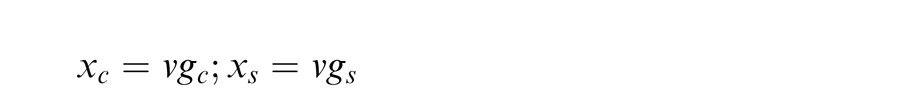 |
The priors on each of the model components are given by:
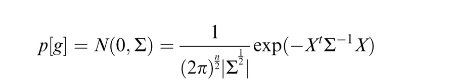 |
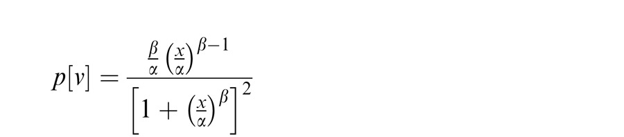 |
We assume α = 1; β = 2. Throughout the paper, we also assume the covariance matrix Σ is the identity matrix.
As in our previous GSM work (Coen-Cagli et al., 2012; Schwartz et al., 2009), we assume that the neural response at a center location is given by the Gaussian estimate for the center. This is obtained via Bayes and given by:
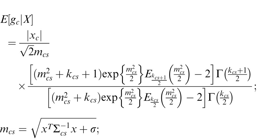 |
(See similar detailed Bayesian derivation in Schwartz et al., 2009 appendix.) Note that this is proportional to a divisive normalization formulation, as pointed out in the main text, with the other terms arising from the usual constraint that the probability distribution must sum to 1:
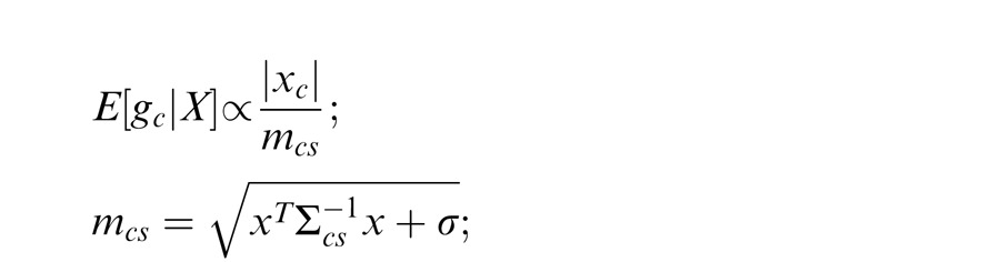 |
where mcs is the gain signal for center and surround (this is the same signal as in the main text, but we write it out more generally with the covariance matrix Σcs); kcs are the number of filters in center and surround; Ei( ) is an exponential integration function; and Γ( ) is the Gamma function.
We can similarly write out the non–co-assigned case, replacing the cs subscripts with c subscripts (since center does not depend on surround and has its own mixer variable).
Posterior co-assignment probability
We estimate the (posterior) probability of co-assignment given the input stimulus and attention weights as follows (using Bayes):
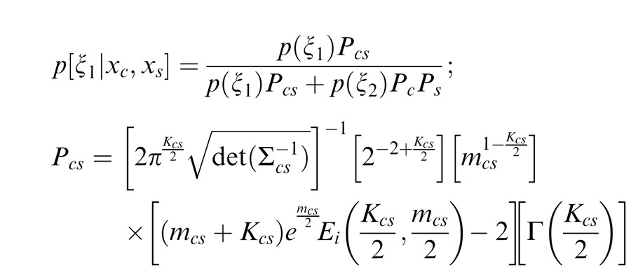 |
We can also similarly write out PcPs, replacing the subscripts cs with c and s respectively, and therefore reflecting the scenario in which center and surround are not co-assigned.
We similarly obtain the (posterior) probability of non–co-assignment, with the two probabilities adding to 1:
 |
These equations are identical for the case of attention, which as before replaces xc to acxc and xs to asxs in all the equations. In this case, the posterior probabilities are defined as p(ξ1 | xc, xs, ac, as) and p(ξ2 | xc, xs, ac, as).
Contributor Information
Odelia Schwartz, Email: odelia.schwartz@einstein.yu.edu.
Ruben Coen-Cagli, Email: Ruben.CoenCagli@unige.ch.
References
- Adelson E. H. (2000). Lightness perception and lightness illusions. In: Gazzaniga M. (Ed.), The new cognitive neurosciences, 2nd Ed, (pp 339–351) Cambridge, MA: MIT Press [Google Scholar]
- Ahmadian Y., Rubin D. B., Miller K. D. (2012). Analysis of the stabilized supralinear network. arXiv:1202.6670v2 [DOI] [PMC free article] [PubMed] [Google Scholar]
- Attneave F. (1954). Some informational aspects of visual perception. Psychological Reviews, 61, 183–193 [DOI] [PubMed] [Google Scholar]
- Ayaz A., Chance F. S. (2009). Gain modulation of neuronal responses by subtractive and divisive mechanisms of inhibition. Journal of Neurophysiology, 101, 958–968 [DOI] [PubMed] [Google Scholar]
- Baluch F., Itti L. (2011). Mechanisms of top-down attention. Trends in Neuroscience, 34(4), 210–224 [DOI] [PubMed] [Google Scholar]
- Barlow H. B. (1961). Possible principles underlying the transformation of sensory messages. In Rosenblith W. A. (Ed.), Sensory communication (pp. 217–234). Cambridge, MA: MIT Press [Google Scholar]
- Bell A. J., Sejnowski T. J. (1997). The ‘independent components' of natural scenes are edge filters. Vision Research, 37, 3327–3338 [DOI] [PMC free article] [PubMed] [Google Scholar]
- Carandini M., Heeger D. J. (2012). Normalization as a canonical neural computation. Nature Reviews Neuroscience, 13, 51–62 [DOI] [PMC free article] [PubMed] [Google Scholar]
- Carrasco M. (2011). Visual attention: The past 25 years. Vision Research, 51, 1484–1525 [DOI] [PMC free article] [PubMed] [Google Scholar]
- Carrasco M., Ling S., Read S. (2004). Attention alters appearance. Nature Neuroscience, 7, 308–313 [DOI] [PMC free article] [PubMed] [Google Scholar]
- Cavanaugh J. R., Bair W., Movshon J. A. (2002). Selectivity and spatial distribution of signals from the receptive field surround in macaque V1 neurons. Journal of Neurophysiology, 88, 2547–2556 [DOI] [PubMed] [Google Scholar]
- Chen Y., Martinez-Conde S., Macknik S. L., Bereshpolova Y., Swadlow H. A., Alonso J. M. (2008). Task difficulty modulates the activity of specific neuronal populations in primary visual cortex. Nature Neuroscience, 11(8), 974–982 [DOI] [PMC free article] [PubMed] [Google Scholar]
- Chikkerur S., Serre T., Tan C., Poggio T. (2010). What and where: A Bayesian inference theory of attention. Vision Research, 50(22), 2233–2247 [DOI] [PubMed] [Google Scholar]
- Clifford C. W. (2002). Perceptual adaptation: Motion parallels orientation. Trends in Cognitive Science, 6(3), 136–143 [DOI] [PubMed] [Google Scholar]
- Clifford C. W. G., Wenderoth P., Spehar B. (2000). A functional angle on some after-effects in cortical vision. Proceedings of the Royal Society of London Series B: Biological Sciences, 267, 1705–1710 [DOI] [PMC free article] [PubMed] [Google Scholar]
- Coen-Cagli R., Dayan P., Schwartz O. (2009). Statistical models of linear and nonlinear contextual interactions in early visual processing. In: Bengio Y., Schuurmans D., Lafferty J., Williams C. K. I., Culotta A. (Eds.), Advances in neural information processing systems (pp 369–377). Cambridge, MA: MIT Press [Google Scholar]
- Coen-Cagli R., Dayan P., Schwartz O. (2012). Cortical surround interactions and perceptual salience via natural scene statistics. PLoS Computational Biology, 8(3), e1002405. [DOI] [PMC free article] [PubMed] [Google Scholar]
- Cohen M. R., Maunsell J. H. (2009). Attention improves performance primarily by reducing interneuronal correlations. Nature Neuroscience, 12, 1594–1600 [DOI] [PMC free article] [PubMed] [Google Scholar]
- Cohen M. R., Maunsell J. H. (2011). Using neuronal populations to study the mechanisms underlying spatial and feature attention. Neuron, 70(6), 1192–1204 [DOI] [PMC free article] [PubMed] [Google Scholar]
- Dayan P. (2009). Load and attentional bayes. Advances in Neural Information Processing Systems, 21, 369–376 [Google Scholar]
- Dayan P., Solomon J. A. (2010). Selective Bayes: Attentional load and crowding. Vision Research, 50(22), 2248–2260 [DOI] [PubMed] [Google Scholar]
- Dayan P., Zemel R. S. (1999). Statistical models and sensory attention. Proceedings of the Ninth International Conference on Artificial Neural Networks , Vol. 2, 1017–1022 [Google Scholar]
- Eckstein M. P., Peterson M. F., Pham B. T., Droll J. A. (2009). Statistical decision theory to relate neurons to behavior in the study of covert visual attention. Vision Research, 49(10), 1097–1128 [DOI] [PubMed] [Google Scholar]
- Festman Y., Braun J. (2012). Feature-based attention spreads preferentially in an object-specific manner. Vision Research, 54, 31–38 [DOI] [PubMed] [Google Scholar]
- Freeman E., Driver J., Sagi D., Zhaoping L. (2003). Top-down modulation of lateral interactions in early vision: Does attention affect integration of the whole or just perception of the parts? Current Biology, 13(11), 985–989 [DOI] [PubMed] [Google Scholar]
- Geisler W. S., Albrecht D. G. (1992). Cortical neurons: Isolation of contrast gain control. Vision Research, 8, 1409–1410 [DOI] [PubMed] [Google Scholar]
- Georgopoulos A. P., Schwartz A. B., Kettner R. E. (1986). Neuronal population coding of movement direction. Nature, 233, 1416–1419 [DOI] [PubMed] [Google Scholar]
- Ghose G. M. (2009). Attentional modulation of visual responses by flexible input gain. Journal of Neurophysiology, 101(4), 2089–2106 [DOI] [PMC free article] [PubMed] [Google Scholar]
- Guerrero-Colon J. A., Simoncelli E. P., Portilla J. (2008). Image denoising using mixtures of Gaussian scale mixtures. In Proceedings of 15th IEEE International Conference on Image Processing, October 2008, San Diego, CA, 565–568 [Google Scholar]
- Hayhoe M. M., Ballard D. H. (2005). Eye movements in natural behavior. Trends in Cognitive Science, 9(4), 188–194 [DOI] [PubMed] [Google Scholar]
- Heeger D. J. (1992). Normalization of cell responses in cat striate cortex. Visual Neuroscience, 9, 181–197 [DOI] [PubMed] [Google Scholar]
- Herrmann K., Montaser-Kouhsari L., Carrasco M., Heeger D. J. (2010). When size matters: Attention affects performance by contrast or response gain. Nature Neuroscience, 13, 1554–1559 [DOI] [PMC free article] [PubMed] [Google Scholar]
- Hinton G. E., Ghahramani Z. (1997). Generative models for discovering sparse distributed representations. Philosophical Transactions Royal Society B, 352, 1177–1190 [DOI] [PMC free article] [PubMed] [Google Scholar]
- Karklin Y., Lewicki M. S. (2005). A hierarchical Bayesian model for learning nonlinear statistical regularities in nonstationary natural signals. Neural Computations, 17, 397–423 [DOI] [PubMed] [Google Scholar]
- Karklin Y., Lewicki M. S. (2009). Emergence of complex cell properties by learning to generalize in natural scenes. Nature, 457(7225), 83–86 [DOI] [PubMed] [Google Scholar]
- Lee J., Maunsell J. H. R. (2009). A normalization model of attentional modulation of single unit responses. PLoS One, 4, e4651. [DOI] [PMC free article] [PubMed] [Google Scholar]
- Liu T., Larsson J., Carrasco M. (2007). Feature-based attention modulates orientation-selective responses in human visual cortex. Neuron, 55(2), 313–323 [DOI] [PMC free article] [PubMed] [Google Scholar]
- Mareschal I., Morgan M. J., Solomon J. A. (2010). Attentional modulation of crowding. Vision Research, 50, 805–809 [DOI] [PubMed] [Google Scholar]
- Maunsell J. H., Treue S. (2006). Feature-based attention in visual cortex. Trends in Neuroscience, 29(6), 317–322 [DOI] [PubMed] [Google Scholar]
- McAdams C. J., Maunsell J. H. (1999). Effects of attention on orientation-tuning functions of single neurons in macaque cortical area V4. Journal of Neuroscience, 19(1), 431–441 [DOI] [PMC free article] [PubMed] [Google Scholar]
- McAdams C. J., Reid R. C. (2005). Attention modulates the responses of simple cells in monkey primary visual cortex. Journal of Neuroscience, 25(47), 11023–11033 [DOI] [PMC free article] [PubMed] [Google Scholar]
- Mishra J., Fellous J. M., Sejnowski T. J. (2006). Selective attention through phase relationship of excitatory and inhibitory input synchrony in a model cortical neuron. Neural Networks, 19(9), 1329–1346 [DOI] [PMC free article] [PubMed] [Google Scholar]
- Mitchell J. F., Sundberg K. A., Reynolds J. H. (2009). Spatial attention decorrelates intrinsic activity fluctuations in macaque area V4. Neuron, 63(6), 879–888 [DOI] [PMC free article] [PubMed] [Google Scholar]
- Moore C. I., Carlen M., Knoblich U., Cardin J. A. (2010). Neocortical interneurons: From diversity, strength. Cell, 142(2), 189–193 [DOI] [PMC free article] [PubMed] [Google Scholar]
- Moran J., Desimone R. (1985). Selective attention gates visual processing in the extrastriate cortex. Science, 229, 782–784 [DOI] [PubMed] [Google Scholar]
- Motter B. C. (1993). Focal attention produces spatially selective processing in visual cortical areas V1, V2, and V4 in the presence of competing stimuli. Journal of Neurophysiology, 70, 909–919 [DOI] [PubMed] [Google Scholar]
- Nauhaus I., Busse L., Carandini M., Ringach D. L. (2009). Stimulus contrast modulates functional connectivity in visual cortex. Nature Neuroscience, 12, 70–76 [DOI] [PMC free article] [PubMed] [Google Scholar]
- Ni A. M., Ray S., Maunsell J. H. (2012). Tuned normalization explains the size of attention modulations. Neuron, 73(4), 803–813 [DOI] [PMC free article] [PubMed] [Google Scholar]
- Olshausen B. A., Field D. J. (1996). Emergence of simple-cell receptive field properties by learning a sparse code for natural images. Nature, 381, 607–609 [DOI] [PubMed] [Google Scholar]
- Prinzmetal W., Nwachuku I., Bodanski L. (1997). The phenomenology of attention 2: Brightness and ontrast. Consciousness & Cognition, 6, 372–412 [PubMed] [Google Scholar]
- Rao R. (2005). Bayesian inference and attentional modulation in the visual cortex. NeuroReport, 16(16), 1843–1848 [DOI] [PubMed] [Google Scholar]
- Rao R. P., Ballard D. H. (1999). Predictive coding in the visual cortex: A functional interpretation of some extra-classical receptive-field effects. Nature Neuroscience, 2, 79–87 [DOI] [PubMed] [Google Scholar]
- Reynolds J. H., Chelazzi L. (2004). Attentional modulation of visual processing. Annual Review Neuroscience, 27, 611–647 [DOI] [PubMed] [Google Scholar]
- Reynolds J. H., Heeger D. J. (2009). The normalization model of attention. Neuron, 61(2), 168–185 [DOI] [PMC free article] [PubMed] [Google Scholar]
- Roberts M., Delicato L. S., Herrero J., Gieselmann M. A., Thiele A. (2007). Attention alters spatial integration in macaque V1 in an eccentricity-dependent manner. Nature Neuroscience, 10, 1483–1491 [DOI] [PMC free article] [PubMed] [Google Scholar]
- Roelfsema P. R., Lamme V. A. F., Spekreijse H. (1998). Object-based attention in the primary visual cortex of the macaque monkey. Nature, 395, 376–381 [DOI] [PubMed] [Google Scholar]
- Salinas E. (2003). Background synaptic activity as a switch between dynamical states in a network. Neural Computation, 15, 1439–1475 [DOI] [PubMed] [Google Scholar]
- Schein S. J., Desimone R. (1990). Spectral properties of V4 neurons in the macaque. Journal of Neuroscience, 10, 3369–3389 [DOI] [PMC free article] [PubMed] [Google Scholar]
- Schwabe L., Obermayer K., Angelucci A., Bressloff P. C. (2006). The role of feedback in shaping the extra-classical receptive field of cortical neurons: A recurrent network model. Journal of Neuroscience, 26, 9117–9129 [DOI] [PMC free article] [PubMed] [Google Scholar]
- Schwartz O., Hsu A., Dayan P. (2007). Space and time in visual context. Nature Reviews Neuroscience, 8, 522–535 [DOI] [PubMed] [Google Scholar]
- Schwartz O., Sejnowski T. J., Dayan P. (2006). Soft mixer assignment in a hierarchical generative model of natural scene statistics. Neural Computation, 18, 2680–2718 [DOI] [PMC free article] [PubMed] [Google Scholar]
- Schwartz O., Sejnowski T. J., Dayan P. (2009). Perceptual organization in the tilt illusion. Journal of Vision, 9(4):19, 1–20, http://www.journalofvision.org/content/9/4/19, doi:10.1167/9.4.19 [PubMed] [Article] [DOI] [PMC free article] [PubMed] [Google Scholar]
- Schwartz O., Simoncelli E. P. (2001). Natural signal statistics and sensory gain control. Nature Neuroscience, 4, 819–825 [DOI] [PubMed] [Google Scholar]
- Simoncelli E. P., Olshausen B. A. (2001). Natural image statistics and neural representation. Annual Review of Neuroscience, 24, 1193–1216 [DOI] [PubMed] [Google Scholar]
- Spivey M. J., Spirn M. J. (2000). Selective visual attention modulates the direct tilt aftereffect. Perception & Psychophysics, 62(8), 1525–1533 [DOI] [PubMed] [Google Scholar]
- Spratling M. W. (2008). Predictive coding as a model of biased competition in visual attention. Vision Research, 48(12), 1391–1408 [DOI] [PubMed] [Google Scholar]
- Sundberg K. A., Mitchell J. F., Reynolds J. H. (2009). Spatial attention modulates center-surround interactions in macaque visual area V4. Neuron, 61(6), 952–963 [DOI] [PMC free article] [PubMed] [Google Scholar]
- Tiesinga P. H., Buia C. I. (2009). Spatial attention in area V4 is mediated by circuits in primary visual cortex. Neural Network, 22(8), 1039–1054 [DOI] [PubMed] [Google Scholar]
- Tiesinga P. H., Fellous J. M., Salinas E., José J. V., Sejnowski T. J. (2004). Synchronization as a mechanism for attentional gain modulation. Neurocomputing, 58–60, 641–646 [DOI] [PMC free article] [PubMed] [Google Scholar]
- Tsal Y., Shalev L., Zakay D., Lubow R. E. (1994). Attention reduces perceived brightness contrast. Quarterly Journal of Experimental Psychology, 47, 865–893 [DOI] [PubMed] [Google Scholar]
- Tsotsos J. K. (2011). A computational perspective on visual attention. Cambridge, MA: MIT Press [Google Scholar]
- Tzvetanov T., Womelsdorf T., Niebergall R., Treue S. (2006). Feature-based attention influences contextual interactions during motion repulsion. Vision Research, 46(21), 3651–3658 [DOI] [PubMed] [Google Scholar]
- Wainwright M. J., Simoncelli E. P. (2000). Scale mixtures of {Gaussians} and the statistics of natural images. In Solla S. A., Leen T. K., Müller K. R. (Eds.), Advances in Neural Information Processing Systems (pp 855–861) Cambridge, MA: MIT Press [Google Scholar]
- Wainwright M. J., Simoncelli E. P., Willsky A. S. (2001). Random cascades on wavelet trees and their use in modeling and analyzing natural imagery. Applied & Computational Harmonic Analysis, 11, 89–123 [Google Scholar]
- Wannig A., Rodríguez V., Freiwald W. A. (2007). Attention to surfaces modulates motion processing in extrastriate area MT. Neuron, 54(4), 639–651 [DOI] [PubMed] [Google Scholar]
- Wannig A., Stanisor L., Roelfsema P. R. (2011). Automatic spread of attentional response modulation along Gestalt criteria in primary visual cortex. Nature Neuroscience, 14(10), 1243–1244 [DOI] [PubMed] [Google Scholar]
- Whiteley L. E. (2008). Uncertainty, reward, and attention in the Bayesian brain. PhD thesis, Gatsby Computational Neuroscience Unit, UCL [Google Scholar]
- Yu A. J., Dayan P. (2005). Inference, attention, and decision in a Bayesian neural architecture. Advances in Neural Information Processing Systems, 17(17), 1577–1584 [Google Scholar]
- Yu A. J., Dayan P., Cohen J. D. (2009). Dynamics of attentional selection under conflict: Toward a rational Bayesian account. Journal of Experimental Psychology: Human Perception & Performance, 35, 700–717 [DOI] [PMC free article] [PubMed] [Google Scholar]
- Zetzsche C., Nuding U. (2005). Nonlinear and higher-order approaches to the encoding of natural scenes. Network, 16(2–3), 191–221 [DOI] [PubMed] [Google Scholar]
- Zhaoping L. (2006). Theoretical understanding of the early visual processes by data compression and data selection. Network: Computation in Neural Systems, 17(4), 301–334 [DOI] [PubMed] [Google Scholar]