Identity by Descent Estimation With Dense Genome-Wide Genotype Data

Abstract

We present a novel method, IBDLD, for estimating the probability of identity by descent (IBD) for a pair of related individuals at a locus, given dense genotype data and a pedigree of arbitrary size and complexity. IBDLD overcomes the challenges of exact multipoint estimation of IBD in pedigrees of potentially large size and eliminates the difficulty of accommodating the background linkage disequilibrium (LD) that is present in high-density genotype data. We show that IBDLD is much more accurate at estimating the true IBD sharing than methods that remove LD by pruning SNPs and is highly robust to pedigree errors or other forms of misspecified relationships. The method is fast and can be used to estimate the probability for each possible IBD sharing state at every SNP from a high-density genotyping array for hundreds of thousands of pairs of individuals. We use it to estimate point-wise and genomewide IBD sharing between 185,745 pairs of subjects all of whom are related through a single, large and complex 13-generation pedigree and genotyped with the Affymetrix 500 k chip. We find that we are able to identify the true pedigree relationship for individuals who were misidentified in the collected data and estimate empirical kinship coefficients that can be used in follow-up QTL mapping studies. IBDLD is implemented as an open source software package and is freely available.

INTRODUCTION

The potential for novel genetic insights afforded by high-density genotyping arrays has spurred a renewed interest in methods for estimating identity by descent (IBD) between pairs of individuals. Estimates of IBD have allowed for the discovery of large scale chromosomal and genomic sharing [Visscher et al., 2006], refined estimates of heritability and genomic partitioning of genetic variance [Visscher et al., 2007], discovery of deletions [Gusev et al., 2009], and, of particular recent interest, the identification and use of short shared segments between distant relatives [Purcell et al., 2007; Browning, 2008; Browning and Browning, 2011, 2010; Huff et al., 2011].

More traditionally, IBD estimates have been used for linkage analysis in families where the IBD estimates have assumed independence between markers [Lander and Green, 1987; Kruglyak et al., 1996; Abecasis et al., 2002; Abecasis and Wigginton, 2005]. This assumption, however, no longer holds with modern genotyping arrays where there may be extensive linkage disequilibrium (LD) between markers. Recent methods that incorporate LD in their estimates of IBD within families are designed for pedigrees of small size Keith et al. [2008]; Kurbasic and Hossjer [2008]. Other approaches that have been used include clustering of tightly linked markers [Abecasis and Wigginton, 2005] or to filter out markers in LD leaving a set of SNPs that can be used in standard software packages, e.g. Bellenguez et al. [2009a]. The first of these approaches can dramatically increase the computational effort while the latter results in large amounts of potentially informative genotype data being discarded.

Loss of information may also happen when large pedigrees are used. Extended pedigrees, though known to have higher power for linkage mapping than small pedigrees [Chapman and Wijsman, 2001], present challenging computational problems [Bellenguez et al., 2009b]. When the pedigrees are too large for exact computation of IBD, one typical strategy is to split the pedigree into multiple smaller subpedigrees [Falchi et al., 2004; Brocklebank et al., 2007; Liu et al., 2008; Bellenguez et al., 2009b]. Treating these subpedigrees as independent may result in a loss of power from ignoring the information that exists between subpedigrees [Dyer et al., 2001]. In some circumstances Markov chain Monte Carlo methods [Sobel and Lange, 1996; Heath, 1997; George and Thompson, 2003; Sung et al., 2007] and approximate IBD estimation algorithms [Almasy and Blangero, 1998] have proven useful, though the effectiveness and properties of these approaches will need further exploration when marker data are extremely dense or pedigrees are very large or complex. Two issues, then, have limited the utility of pedigrees, particularly extended pedigrees, for IBD-based mapping, (1) the challenges of doing computations with high degree or complexly related relatives, and (2) the difficulties of using dense marker data with high LD between markers. Here, we present a computationally efficient method that overcomes both of these problems, allowing estimation of multipoint IBD between pairs of arbitrarily related individuals using high-density genetic markers.

The method we present, referred to as IBDLD, is based on a hidden Markov model (HMM) of IBD between pairs of individuals but with modifications to incorporate LD in the observed genotype probabilities. IBDLD can build a background LD model based on a panel of either phased haplotypes or unphased genotypes and is fast enough to estimate IBD at hundreds of thousands of SNPs for hundreds of thousands of pairs. We consider two models for background LD. The first model requires individuals in the panel be phased, with the background LD modeling based on two-locus haplotype frequencies. This approach was recently used by Albrechtsen et al. [2009]. The second model requires only unphased genotypes in the panel and uses a multilocus model of LD. Below, we demonstrate the accuracy of IBDLD using simulations in both sibling pairs and pairs of individuals related through a large, complex genealogy. We also analyze a real data set consisting of 185,745 pairs (609 individuals) all of whom were typed with the Affymetrix 500 k chip and are related through a 13 generation, 3,555 person pedigree. Finally, we discuss the utility of the method and implications for complex trait mapping.

MATERIAL AND METHODS

HMMs are effective tools for estimating IBD in small to medium-sized families [Lander and Green, 1987; Kruglyak et al., 1996; Abecasis et al., 2002], as well as providing a useful approximation in larger pedigrees [Thompson, 1994; McPeek and Sun, 2000; Abney et al., 2002], but their continuing utility in the era of dense marker data will necessarily rely on a computationally efficient method that incorporates LD that may extend over a distance that encompasses many markers. Below we briefly review the standard HMM before describing our extensions to include LD.

STANDARD HMM

The model described here is essentially identical to the HMM used in the PLINK [Purcell et al., 2007] software package to identify IBD segments in pairs of individuals. Because we wish to estimate IBD between pairs of individuals joined by a known pedigree while allowing for inbreeding, we define the hidden state variable S_i at marker i to take on values 1,…,9 according to which of the condensed identity states [Jacquard, 1974] describes the IBD sharing between the pair (see Fig. 1). Computation in the HMM depends on three probabilities (1) the condensed identity state probability at the first marker, (2) the transition probabilities between states and (3) the probabilities of the observations given the underlying state. The condensed identity state probability at the first marker P(S₁ = r) is equal to the prior probabilities for each condensed identity state (i.e. depending only on the known pedigree) given by quantities Δ₁,…,Δ₉. We model the sequence of IBD states at L markers S₁,…,S_L with a Markov chain with the resultant property that conditional on S_i, the distribution of the state at marker i+1 depends only on the transition probability matrix T_rt = P(S_i+1 = t|S_i = r). Though the IBD states are not, in fact, Markov, this approximation has proven effective in previous studies [Thompson, 1994; McPeek and Sun, 2000; Abney et al., 2002]. The final element of the HMM are the emission probabilities which give the probabilities of the genotypes of the pair given their underlying condensed identity state P(G_i|S_i). With these probabilities specified it is straightforward to use the forward–backward algorithm [Baum, 1972] to estimate the probabilities of each condensed identity state at an arbitrary point of the chromosome given all the observed genotype data for that pair.

Fig. 1.

The condensed identity states. The 15 possible detailed identity states for individuals A and B, grouped according to their nine condensed states. Points represent alleles and lines indicate alleles that are IBD.

The transition probabilities depend on both the genetic distance between the markers as well as the pedigree connecting the pair under consideration. We propose estimating the transition probabilities in the following way. Let ${\mathrm{S}}_i^T=(1_{S_i=1},\dots ,1_{S_i=9})$ be a vector whose elements are indicator functions of the IBD state at position i. Then the probability distribution at marker i+1 is $P\left({\mathrm{S}}_{i+1}^T\right)=P\left({\mathrm{S}}_i^T\right)\mathrm{T}(x_{i+1}-x_i)$, where T(x) is the transition probability matrix for genetic distance x. Because we assume the hidden states form a Markov chain, the transition matrix can be written T(x) = e^Qx where Q is the infinitesimal rate matrix. Note that T(x) = UD(x)U⁻¹, where U is a matrix whose columns are the eigenvectors of Q and D(x) = diage(e^λ₁x,…,e^λ₁x,…,e^λ₉x) where eigenvalue λ₁ is the lth eigenvalue of Q and 0 = λ₁ ≥ … ≥ λ₉. Hence, T_rt(x), the probability of transitioning from state r to t over distance x, can be written in the form

$$T_{\mathit{rt}}\left(x\right)=\sum _{l=1}^9{a}_{l,\mathit{rt}}{e}^{{\lambda }_{l}x}.$$ (1)

The elements of the transition matrix, T_rt are subject to the following boundary conditions:

$$T_{\mathit{rt}}\left(0\right)=\left\{\begin{array}{cc}0\hfill & r\ne t\hfill \\ 1\hfill & r=t\hfill \end{array}\phantom{\}}\text{and}\underset{x\to \infty }{\lim }{T}_{\mathit{rt}}\right(x)={\Delta }_t.$$ (2)

We approximate the transition probabilities in Equation (1) with a single exponential term,

$$T_{\mathit{ij}}\left(x\right)\approx a_{1,\mathit{ij}}+a_{2,\mathit{ij}}{e}^{\lambda x},$$ (3)

which, combined with the boundary conditions (Equation (2)), gives a_1,ij = Δ_j and a_2,ij = −Δ_j for i≠j or a_1,ii =Δ_i and a_2,ii = 1 – Δ_i for i = j. Note that the parameters a_l and λ are specific to the pair of individuals. This model is equivalent to one where the next state entered is drawn from the stationary distribution.

The emission probabilities are the probabilities of the true genotypes for the pair of individuals given their underlying condensed identity state at locus i, P(G_i|S_i), where $G_i=(G_i^1,G_i^2)$ are the true genotypes for the pair. Here we assume that all markers are biallelic SNPs with allelic types 0 and 1, and denote the genotype of person p, $G_i^p$, as 0, 1, or 2. These emission probabilities depend on the allele frequency at the locus and are readily computed for each condensed identity state and are given in Supplementary Table S1 [Abney, 2008]. Actual observations of the genotypes, however, may differ from the true underlying genotypes due to errors or missing data. We, therefore, include an additional set of probabilities allowing us to model these effects. We let $O_i=(O_i^1,O_i^2)$ be the observed genotypes at marker i for the two individuals and M = (M¹,M²) to be the set of missing genotypes for that pair. We condition all observations on the set of missing genotypes, which amounts to assuming that the missing value mechanism is independent of the underlying genotype, resulting in $P(O_i^p=-\mid M^p)=1$, where “–” represents a missing genotype. To allow for genotyping error we introduce the parameter ε and use the probabilities as shown in Supplementary Table S2.

MODELING LD

The standard HMM ignores the dependence between genotypes that exists in the presence of LD. Below, we modify the HMM so that the emission probabilities P(G_i|S_i) at SNP i depend on the genotypes at previous loci. Extending the HMM to use conditional emission probabilities can greatly add to the computational burden, if one were to attempt to exactly model the LD in the entire set of SNPs. Our focus is to model the LD as completely as possible while still keeping the computations tractable. In general, modeling LD requires a large enough set of individuals from the population from which the pattern of dependence between loci can be estimated. We term this set of individuals the “training” sample, and they are used to obtain estimates of the parameters in our LD model. Below, we describe two LD models that we have implemented. The first can be used when the training sample has completely phased genotypes, while the second can be used even when phase is unknown. In both cases, as in the standard HMM, the sample of individuals within whom we wish to estimate IBD need not be phased.

Modeling LD: conditioning on a single SNP genotype

We modify the emission probabilities using an approach developed by Albrechtsen et al. [2009]. In this model we condition the current genotype probability on the genotype and condensed identity state at a single previous marker, P(G_i|G_h, S_i = S_h = s), where i is the current marker, h is a previous marker and s is the current condensed identity state. We obtain the joint probability of the genotypes at the two loci given a condensed identity state P(G_i, G_h|S_i = S_h = s) by summing over all possible phasings of the genotypes using Supplementary Table S1 for the genotype probabilities given a particular phasing. In this case, the allele frequencies in Supplementary Table S1 should be interpreted as haplotype frequencies. For instance, if two individuals were both heterozygote (0,1) at both loci h and i, conditional on condensed identity state 7, we would obtain the joint probability P(G_h, G_i|S_h = S_i = 7) = 2f₀₀f₁₁+2f₀₁f₁₀, where f_x is the frequency of haplotype x. The final emission probabilities for the observed genotype at locus i are

$$\begin{array}{cc}\hfill & P(O_i\mid O_h,S_i=S_h=r,\epsilon )\hfill \\ \hfill & =\frac{P(O_i,O_h\mid S_i=S_h=r,\epsilon )}{P(O_h\mid S_h=r,\epsilon )}\hfill \\ \hfill & =\frac{{\Sigma }_{G_i{G}_h}P(G_i,G_h\mid S_i=S_h=r)\left({\Pi }_{l=1}^{2}P\right(O_i^l\mid G_i^l,\epsilon \left)\right)\left({\Pi }_{l=1}^{2}P\right(O_h^l\mid G_h^l,\epsilon \left)\right)}{{\Sigma }_{G_h}P(G_h\mid S_h=r)\left({\Pi }_{l=1}^{2}P\right(O_h^l\mid G_h^l,\epsilon \left)\right)}.\hfill \end{array}$$

It is possible that between loci h and i the Markov process has made a transition to a different state. In this case we now assume that the emission probability at locus i is conditionally independent of the genotype and state at locus h,

$$\begin{array}{cc}\hfill P& (O_i\mid O_h,S_i\ne S_h,S_i=r,\epsilon )\hfill \\ \hfill & =P(O_i\mid S_i=r,\epsilon )=\sum _{G_i}P(G_i\mid S_i=r)\left(\prod _{l=1}^{2}P(O_i^l\mid G_i^l,\epsilon )\right).\hfill \end{array}$$

We note that, as in Albrechtsen et al. [2009], we do not necessarily choose locus h to be the marker immediately preceding i. Below, we consider the two cases where it is either the immediately preceding marker or the marker with highest correlation, in the training sample, to marker i among the L previous markers within a specified distance.

Modeling LD: conditioning on multiple SNP genotypes

The above procedure for modeling LD should be effective when the allele at SNP i on a given haplotype is conditionally independent of the other markers on that haplotype given the allele at SNP h. This may often be approximately true when the LD between the two SNPs is sufficiently large, but may be less accurate when pairwise LD is small yet there is strong dependence given the alleles at multiple loci. Extending the above model to include L rather than one previous marker would require summation over 2^L+1 possible haplotype phases to get the joint genotype probability for the L markers for the two individuals. Doing this across the genome can quickly become computationally intractable as L increases above one. Instead, we propose a novel method that approximates the LD structure through a linear model. This has the advantage of maintaining computational efficiency in spite of the underlying complexity, allows the use of unphased data—a particular advantage when obtaining fully phased data may be either difficult or impractical, in pedigrees for instance—and, as we show in the Results, accurately corrects the HMM in the presence of LD.

To motivate our approach consider the conditional probability of individual 1 having genotype 0 at marker i given the genotype at locus i–1,

$$\begin{array}{cc}\hfill P(G_i^1=0\mid G_{i-1}^1)& =P(G_i^1=0\mid G_{i-1}^1=0)1_{G_{i-1}^1=0}\hfill \\ \hfill & +P(G_i^1=0\mid G_{i-1}^1=1)1_{G_{i-1}^1}=1\hfill \\ \hfill & +P(G_i^1=0\mid G_{i-1}^1=1)1_{G_{i-1}^1}=2\hfill \\ \hfill & ={\gamma }_{i,0}+{\gamma }_{i-1,00}{1}_{G_{i-1}^1=0}+{\gamma }_{i-1,20}{1}_{G_{i-1}^1=2},\hfill \end{array}$$

where 1_x is the indicator function equaling one when event x is true and is zero otherwise. In this case we have ${\gamma }_{i,0}=P(G_i^1=0\mid G_{i-1}^1=1),{\gamma }_{i-1,00}=P(G_i^1=0\mid G_{i-1}^1=0)-P(G_i^1=0\mid G_{i-1}^1=1),{\gamma }_{i-1,20}=P(G_i^1=0\mid G_{i-1}^1=2)-P(G_i^1=0\mid G_{i-1}^1=1)$. We propose extending this linear model as an approximate way to include the effects of LD across L loci. We first define a representation for the genotype of individual p at a locus i in terms of indicator functions, ${\tilde{G}}_i^p={(1_{G_i^p=0},1_{G_i^p=2})}^t$. We then have

$$\begin{array}{cc}\hfill P({\tilde{G}}_i^p\mid {\tilde{G}}_{i-1}^p,\dots ,{\tilde{G}}_{i-L}^p)& =\left(\begin{array}{c}\hfill P(G_i^p=0\mid G_{i-1}^p,\dots ,G_{i-L}^p)\hfill \\ \hfill P(G_i^p=2\mid G_{i-1}^p,\dots ,G_{i-L}^p)\hfill \end{array}\right)\hfill \\ \hfill & =\left(\begin{array}{cc}\hfill 1\hfill & \hfill 0\hfill \\ \hfill 0\hfill & \hfill 1\hfill \end{array}\right)\left(\begin{array}{c}\hfill {\gamma }_{i,0}\hfill \\ \hfill {\gamma }_{i,2}\hfill \end{array}\right)+\left(\begin{array}{cc}\hfill {\gamma }_{i-1,00}\hfill & \hfill {\gamma }_{i-1,20}\hfill \\ \hfill {\gamma }_{i-1,02}\hfill & \hfill {\gamma }_{i-1,22}\hfill \end{array}\right){\tilde{G}}_{i-1}^p\hfill \\ \hfill & +\dots +\left(\begin{array}{cc}\hfill {\gamma }_{i-L,00}\hfill & \hfill {\gamma }_{i-L,20}\hfill \\ \hfill {\gamma }_{i-L,02}\hfill & \hfill {\gamma }_{i-L,22}\hfill \end{array}\right){\tilde{G}}_{i-L}^p.\hfill \end{array}$$ (4)

We additionally impose lower and upper bounds of 0.01 and 0.99, respectively, on the predicted probabilities $P({\tilde{G}}_i^p\mid {\tilde{G}}_{i-1}^p,\dots ,{\tilde{G}}_{i-L}^p)$. From the above we can readily compute the probability of the heterozygote from $P(G_i^p=1\mid G_{i-1}^p,\dots ,G_{i-L}^p)=1-P(G_i^p=0\mid G_{i-1}^p,\dots ,G_{i-L}^p)-P(G_{i-1}^p=2\mid G_{i-1}^p,\dots ,G_{i-L}^p)$. It should be noted that in this multilocus linear model the γ parameters no longer have the simple probability interpretation they do in the two locus case.

Equation (4) provides an efficient framework for determining the genotype frequencies at a locus given the genotypes at previous loci in an individual. The emission probabilities require the joint genotype probabilities of two individuals at a locus given the underlying condensed identity state. Supplementary Table S1 provides these probabilities given the allele probabilities at a locus. To use these probabilities we have to convert the genotype probabilities obtained from Equation (4) for each subject into an equivalent, subject-specific allele probability. A difficulty with this approximation, however, is that the joint genotype probabilities in Supplementary Table S1 assume a common allele probability for both individuals, which is not the case here. For example consider two individuals both homozygous for allele 0. Conditional on the individuals being in condensed identity state S = 1 at that locus the probability P(G¹ = 0; G² = 0|S = 1) = f₀, where f₀ is the probability of allele 0. In our treatment, these individuals may have different genotypes at previous loci and, hence, different probabilities for allele 0, leaving it unclear what value to use for f₀. We formulate our solution to this in the following way. Define the quantities p_g and q_g as the probability of genotype g = 0,1 or 2 for the two individuals A and B, respectively, where the genotype probabilities are computed conditional on the genotypes at previous loci, as described above. The allele probabilities in person A are e₀ = p₀+(1/2)p₁ for allele 0 and e₁ = p₂+(1/2)p₁ for allele 1, and similarly for person B with allele probabilities f₀ and f₁. For an allele a that is shared IBD between the two individuals, the joint genotype probabilities conditional on the genotypes at previous loci is given by a function M[h₁(e_a), h₂(f_a)] of the frequencies in the two individuals for the allele that is IBD. The functions h₁,h₂ are determined from conditional probability arguments and are derived explicitly in the Supplementary Text. For the function M(,), we considered min(,), max(,), and mean(,) and, based on simulations (data not shown) we found that the highest accuracy was achieved with min(,). The complete set of joint genotype probabilities is given in Supplementary Table S3. For instance, in the above example, where A and B are in condensed identity state S = 1, we obtain the joint conditional probability at locus i $P(G_i^1=0,G_i^2=0\mid S=1,G_{i-1,\dots ,}{G}_{i-L})=M(e_0,f_0)$, where M is the min(,) function. To allow for error we assume the observed genotype at marker i depends on the true genotype and use the same error model described above. For simplicity, we assume that the genotypes at the previous markers we condition on are observed without error. The final emission probability, including the genotyping error rate, is

$$\begin{array}{cc}\hfill P& (O_i\mid G_{i-1,\dots ,}{G}_{i-L,}{S}_i=r,\epsilon )\hfill \\ \hfill & =\sum _{G_i}P(G_i\mid G_{i-1,\dots ,}{G}_{i-L,}{S}_i=r)\left(\prod _{l=1}^{2}P(O_i^l\mid G_i^l,\epsilon )\right).\hfill \end{array}$$

Using this emission probability, it is straightforward to use Baum’ forward-backward algorithm [Baum, 1972] to estimate the probabilities for each condensed identity state at a locus.

ESTIMATING PARAMETERS

Implementation of the HMM to estimate IBD probabilities conditional on multilocus genotype information requires, for each pair, estimates of the unconditional condensed identity state probabilities Δ_j, transition rate parameter λ and background LD parameters γ or two-locus haplotype frequencies. The condensed identity state probabilities are computed from a pedigree using known algorithms [Karigl, 1981; Lange and Sinsheimer, 1992; Abney, 2009].

Estimates of the transition rate λ can also be computed from the known pedigree. Although an exact computation is, in principle, possible for arbitrary pedigrees we use a simpler Monte Carlo approach. To estimate λ in Equation (3) we assign every founder a pair of unique chromosomes and allow the chromosomes to segregate through the pedigree, repeating this procedure 100,000 times. For a given pair in the pedigree, we are then able to estimate the transition probability for the pair being in condensed identity states r and t at loci separated by a genetic distance x. We determine these probabilities for distances from 0 to 1.0 cM in increments of 0.0001 cM. We then find the value $\widehat{\lambda }$ that minimizes the residual sum of squares between the expected and observed transition probabilities.

In our modified HMMs that model LD, we require either haplotype frequencies, for the LD model that conditions on the genotype of a single SNP, or estimates of the coefficients γ in the linear model of Equation (4) when conditioning on multiple SNP genotypes. To estimate haplotype frequencies, we assume a training data set consisting of phased genotype data across all markers of interest. From this sample, we compute the correlation between all pairs of SNPs on each chromosome. Beginning with the second SNP on a chromosome, for each SNP we select the single SNP, from among the L previous SNPs within the genetic distance of D cM, with highest correlation to the current SNP. For this pair of SNPs we compute the haplotype frequencies from the training sample.

Given a linear model, estimating the γ parameters can readily be done using standard linear regression on the training sample. In the context of the HMM, however, the purpose of the linear model is to predict the genotype probabilities at a locus given the genotypes at L previous loci. A difficulty with linear regression in this case is that it is susceptible to overfitting, leading to poor predictions. Shrinkage methods, such as ridge regression, often show superior performance for this type of problem [Hastie et al., 2009]. We use ridge regression with the bivariate linear model of Equation (4) to obtain estimates $\widehat{\gamma }$. We choose the ridge penalty for each marker by doing five-fold cross-validation using the “one-standard-error” rule (i.e. we pick the most parsimonious model within one standard error of the minimum prediction error).

SIMULATIONS

We performed simulations to assess the performance of our methods. We considered two pedigree types. The first was a nuclear family with a sibling pair, and the second was a large, complex 13-generation pedigree, with 70 founders, comprising 3,555 individuals from the Hutterite population (this is an updated version of the pedigree described in Abney et al. [2000]). In the large pedigree the results were evaluated in three pairs of individuals with three different kinship coefficients of 0.051, 0.275 and 0.518, with the last of these being a pair consisting of a person with himself.

To generate genotype data with a realistic LD structure we used the CEU haplotypes from the HapMap project [International Hapmap Consortium et al., 2007]. We created a population of phased chromosomes from the CEU HapMap data by removing haplotypes that were from non-founder individuals, resulting in 234 phased haplotypes, and only using markers that were also present on the 500 k Affymetrix gene chip. We only used SNPs from chromosome 8 that had minor allele frequency greater than 0.05, resulting in 11,643 total SNPs with inter-marker genetic map distances as provided by the HapMap project. For each pedigree we simulated genotypes in the study sample by assigning each founder of the pedigree a pair of randomly selected phased chromosomes from the population. Note that chromosomes were drawn without replacement to reduce the possibility of IBD sharing in the founders. Any relatedness between founders in the CEU population was small and infrequent enough to not noticeably impact our results. The founder chromosomes were allowed to segregate through the pedigree until all individuals in the study sample had genotype data. Phase information in the study sample was ignored. This procedure was repeated 1,000 times for both the sibling and large pedigree pairs. In addition, for each of these 1,000 replicates, we considered two genotype data sets with the first being the simulated genotypes at all markers (i.e. no genotyping error or missing data) and another where each genotype was assigned an incorrect value with 2% probability and a missing value with 5% probability.

HUTTERITE DATA

In addition to our simulation studies, we also used real genotype data from a collection of 609 Hutterite individuals, all of whom are related through a complex 13 generation, 3,555 person pedigree. This population has been described previously [Hostetler, 1974; Abney et al., 2000; Ober et al., 2001]. These individuals were genotyped with the Affymetrix 500 k GeneChip array resulting in genotypes at 237,902 SNPs following quality control procedures [Coop et al., 2008].

RESULTS

Throughout our analyses we compared five methods for computing multipoint IBD estimates. The first method, labeled NoLD, used the standard HMM as described in the Methods section “Standard HMM” with no adjustment for LD among the markers. Our second method is identical to the NoLD method but uses a sparser set of markers; we label this method NoLD-S. For NoLD-S, we randomly selected a set of markers that were separated by one centiMorgan. Both the NoLD and NoLD-S methods use the HMM that is essentially equivalent to the one used in the PLINK software package [Purcell et al., 2007] for identifying IBD segments. Method three included LD in the model as described in the Methods section “Modeling LD: Conditioning on a single SNP genotype” where genotype probabilities at the current marker were conditioned on the genotype at only the immediately previous marker (labeled LD-1). Our fourth method uses the same model as in LD-1, but conditions on the single previous marker with highest correlation to the current marker, from among the 20 previous markers within 2 cM (LD-20). Finally, we used the linear model with ridge regression, as described in the Methods section “Modeling LD: Conditioning on multiple SNP genotypes” to account for LD with L = 20. We call this method LD-RR. In addition to these five methods, for the simulated data in the sib pair, we also estimate IBD using MERLIN [Abecasis et al., 2002; and MERLIN with clusters [Abecasis and Wigginton, 2005] (MERLIN-CL).

We look at two measures of accuracy when comparing the methods. Our first is an overall measure of IBD sharing across all markers. For a pair of individuals we compute the bias and the root mean squared error (RMSE) between the true IBD and estimated IBD sharing, across all loci, where the IBD sharing at a locus is the proportion of alleles shared at that locus. That is, at locus k, the true proportion of alleles shared IBD is ${\pi }_k=1_{S_k=1}+\frac{1}{2}(1_{S_k=3}+1_{S_k=5}+1_{S_k=7})+\frac{1}{4}{1}_{S_k=8}$, where 1_Sk=r is the indicator function of the pair being in condensed identity state r at locus k. The estimated proportion of alleles shared IBD is ${\widehat{\pi }}_k=P(S_k=1\mid G)+\frac{1}{2}\left[P\right(S_k=3\mid G)+P(S_k=5\mid G)+P(S_k=7\mid G\left)\right]+\frac{1}{4}P(S_k=8\mid G)$, where the probabilities are estimated using one of the methods listed above. The average true and estimated proportion of alleles IBD across K loci are $\pi =\frac{1}{K}{\Sigma }_{k=1}^K{\pi }_k$ and $\widehat{\pi }=\frac{1}{k}{\Sigma }_{k=1}^K{\widehat{\pi }}_k$ respectively. We use T replication to measure the bias and RMSE of each method where

$$\text{Bias}=\frac{1}{T}{\Sigma }_{t=1}^T({\widehat{\pi }}^{\left(t\right)}-{\pi }^t)\text{and}\mathrm{RMSE}=\sqrt{\frac{1}{T}{\Sigma }_{t=1}^T{({\widehat{\pi }}^{\left(t\right)}-{\pi }^{\left(t\right)})}^2}.$$

SIBLING PAIRS

We computed the bias and RMSE of the IBD estimating methods described above using the CEU haplotypes to estimate background LD for those methods that allow for it. When using the MERLIN methods, for the data with 2% genotype error and 5% missing data, we first use MERLIN’s genotyping error detection methods to remove genotypes that are flagged as problematic. Figure 2 shows how the chromosome-wide estimates of the average proportion of alleles shared IBD compares with the true values. There is high concordance between estimated and true values for methods that account for LD, though MERLIN-CL does less well in the presence of missing data and genotyping error. We note that the methods that do not include LD show a systematic positive bias when the true sharing is low. Thinning the genotype data to include markers with little or no LD improves the bias but introduces greater variance in the estimates of average IBD. Methods that include LD all show accurate estimates, even in the presence of errors and missing data. The MERLIN-based methods, however, show significant degradation in accuracy when errors are present. Figure 3 and Supplementary Table S4 shows the biases and RMSE of the different methods. We see that NoLD, NoLD-S and MERLIN have higher bias and RMSE than the methods that include LD in the model. Of the methods that include LD, both LD-20 and LD-RR have relatively small bias and RMSE in both missing data and genotyping error scenarios. In addition, the Supplementary Text and Figures show how well each method does at giving high probability to the true IBD state at a locus.

Fig. 2.

Estimated average proportion of alleles shared IBD against the true average proportions for sibling pairs. For each method we consider the two cases where the genotype data (1) have neither missing data nor error, and (2) have 5% missing data and 2% error.

Fig. 3.

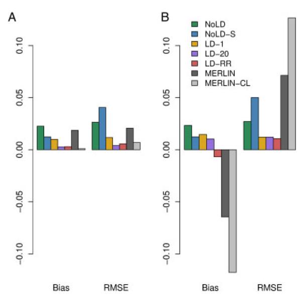
Bias and RMSE for the different methods in a sibling pair. The genotype data (A) have neither missing data nor error, and (B) have 5% missing data and 2% error.

LARGE PEDIGREE PAIRS

As in the simulated sibling pair data, we estimated the LD parameters using the HapMap CEU founder genotypes. As seen in Figure 4 and Supplementary Table S4, the RMSE show a pattern similar to what was seen in the sibling pairs with the methods that model LD having higher accuracy at measuring overall chromosome-wide sharing. In the models that do not include LD, the thinning strategy resulted in much more accurate sharing estimates than did the method that includes all markers. This is likely because in distantly related relative pairs relatively fewer regions are shared IBD, yet the high degree of LD in the dense SNP data results in a larger fraction of regions that are not IBD appearing to be IBD. Similarly, by conditioning on the SNP with the highest LD rather than simply the neighboring SNP, the LD-20 method achieves higher accuracy than the LD-1 method. The LD-RR method is very similar to LD-20 when there are no errors or missing data but shows improved performance when errors and missing data are present. The estimated versus true chromosome-wide proportion of alleles shared IBD for each method are shown in Figure 5 where we see that the models that incorporate LD are able to accurately recover the true chromosome-wide IBD sharing. In addition, the Supplementary Text and Figures show how well each method does at assigning high probability to the true IBD state at a locus.

Fig. 4.

Bias and RMSE for the different methods in the large pedigree pairs. The genotype data (A) have neither missing data nor error, and (B) have 5% missing data and 2% error.

Fig. 5.

Estimated average proportion of alleles shared IBD against the true average proportions for large pedigree pairs. For each method we consider the two cases where the genotype data (1) have neither missing data nor error, and (2) have 5% missing data and 2% error.

TIMING

The standard HMM is computationally efficient, allowing one to include very large numbers of markers in an analysis. Extending the HMM to include LD, however, does impose an extra computational burden, particularly if one wants to adjust for LD using information from many, as opposed to a single marker. The IBDLD method can be broken down into three separate computational tasks, (1) estimating the transition rate parameter λ; (2) estimating the background LD parameters, either γ or the two-locus haplotype frequencies; and (3) estimating IBD for many markers in a pair of individuals. In our large pedigree case, accomplishing task (1) for a single pair took 172 sec using 100,000 simulations. Estimates of the LD parameters were based on 234 phased chromosomes for methods LD-1 and LD-20, and on unphased genotypes from 117 subjects for method LD-RR. For a chromosome with 11,643 SNPs, these estimates took 43.35, 85.05 and 1490.81 sec, respectively. Note that unless a phased panel is already available, methods LD-1 and LD-20 would require additional time to phase the LD training panel. We recorded the time to estimate IBD across the chromosome for each of the methods for a single pair. These results are shown in Table I.

TABLE I.

Method speeds for a single pair for a single chromosome

Method	Missing rate	Error rate	Sibling pair time (sec)	Large pedigree pair time (sec)
NoLD	0	0	0.940	1.020
	0.05	0.02	0.941	1.050
NoLD-S	0	0	0.013	0.014
	0.05	0.02	0.013	0.014
LD-1	0	0	1.657	1.729
	0.05	0.02	1.659	1.731
LD-20	0	0	1.657	1.730
	0.05	0.02	1.658	1.732
LD-RR	0	0	1.337	1.408
	0.05	0.02	1.345	1.411
MERLIN	0	0	0.308	–
	0.05	0.02	0.384	–
MERLIN-CL	0	0	108.360	–
	0.05	0.02	1,913.580	–

HUTTERITE DATA

We obtained estimates for the HMM transition rate parameter λ for each pair of individuals as described in the Methods section. The estimates of $\widehat{\lambda }$ gave exponential curves for the transition probabilities that matched the simulated data extremely well, the mean coefficient of determination across 185,745 pairs was 0.9988 with SD 0.0015.

We applied both methods LD-20 and LD-RR to the Hutterite data. Because the Hutterites are a European-derived population, we estimated the background LD parameters using either the CEU phased founder haplotypes for the LD-20 method, or the CEU unphased founder genotypes for the LD-RR method. We then estimated the genomewide average proportion of alleles shared IBD for all pairs of individuals and compared these estimates to the kinship coefficients as computed from the known pedigree. Assuming no pedigree errors, we expect the genomewide sharing to approximately equal the kinship coefficient with variability resulting from the stochastic nature of segregation. Figure 6A displays the estimated genomewide average proportion of alleles shared IBD as a function of the pair’s kinship coefficient. Both LD-20 and LD-RR plots are very similar (data not shown). The plot shows a high degree of bias in the estimates. We conjecture this is the result of genetic drift in the allele and haplotype frequencies between the ancestral Hutterite population and the current CEU population. To adjust for this effect, we then used the Hutterite genotype data as its own LD training sample. For the LD-RR method we used the genotypes of all the individuals to estimate the LD parameters. To estimate the LD parameters in the LD-20 method we used the 176 phased haplotypes that were previously determined [Coop et al., 2008]. These haplotypes were only phased for SNPs that were completely informative in nuclear families, resulting in haplotypes with a high degree of missing data. Estimating the LD parameters requires enough haplotypes with non-missing data to get a reliable estimate of frequencies. To get good haplotype frequency estimates we imputed missing phase data using the weighted k-nearest neighbor method [Yu and Schaid, 2007] with k = 10, after removing 3,881 SNPs with unphased data greater than 20%. Estimates of the genomewide average proportion of alleles shared IBD against the kinship coefficient are shown in Figure 6B and C. The square root of the mean squared difference between the sharing estimates and the kinship coefficients were 0.0105 and 0.0119 with bias −0.0065 and 0.0080 for the LD-RR and LD-20 methods, respectively.

Fig. 6.

Estimated average proportion of alleles shared IBD across the genome against kinship coefficient for the Hutterite sample. (A) LD-20 using the CEU population to model background LD, (B) LD-20 using the Hutterites themselves to model background LD, (C) LD-RR using the Hutterites themselves to model background LD.

We note that points that lie far off the line in Figure 6 represent pairs with misspecified relationships, either due to errors in the pedigree or sample switches. In particular we note that one pair that was entered into the pedigree as siblings was estimated to have sharing consistent with identical twins. Another pair which the pedigree showed as being distantly related (kinship coefficient <0.05) also had sharing consistent with being identical twins. Further follow-up indicated that a sample had been mistakenly duplicated and assigned incorrectly to another individual in the pedigree. The majority of the other outlying points are pairs involving this incorrectly duplicated individual where the estimated sharing is actually consistent with the true relationship. We also ran PREST [McPeek and Sun, 2000] on the data (Fig. 7), which shows some evidence of misspecified relationships. Inferring the true relationship from the computed EIBD statistic, however, would be difficult for most of the misspecified pairs.

Fig. 7.

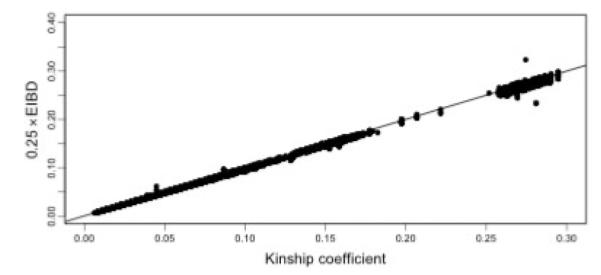
EIBD versus kinship coefficient for the Hutterite sample. Deviations from the diagonal indicate possible pedigree errors. EIBD was computed using PREST.

DISCUSSION

In this work we developed a method, IBDLD, that can rapidly estimate IBD sharing between pairs of individuals related through an arbitrary pedigree given dense genotype data. The problem of estimating IBD in large pedigrees given multipoint genotype data has been a particularly vexing one to geneticists resulting in a variety of pedigree splitting strategies. All such approaches, however, necessarily entail a loss of information which can either lead to a significant reduction in power [Dyer et al., 2001] or increase in false positives [Newman et al., 2001] when performing mapping. These difficulties have been compounded recently with the wide use of genotyping chips with high-density genotyping data. The presence of LD in such data has the consequence of rendering the standard HMM inappropriate. IBDLD overcomes both difficulties and is computationally efficient enough to use genomewide on samples of at least several hundred related individuals.

When using an HMM model that does not incorporate LD, the two methods NoLD and NoLD-S represent two extreme SNP pruning strategies, no pruning and severe pruning, respectively. Other, more sophisticated pruning strategies could be used which would result in accuracy intermediate between the two extremes, while keeping computation time to a minimum. Our results indicate, however, that regardless of the pruning strategy used, accuracy will be far worse than methods that incorporate LD into the model, at the cost of additional computation time.

We explore two different models for including the background LD. Results from the two models indicate that they generally perform similarly, though the LD-RR method appears to be somewhat more robust than LD-20 in the presence of missing genotypes and genotyping error. Additionally, the LD-20 method requires phased haplotypes in the panel of individuals from whom the background LD will be modeled. Although if such a panel is available this does not pose any difficulty, it may often be the case that there is no such suitable data. Using a panel that accurately represents the LD in the study sample is critical to the accuracy of the method. In the analysis of the Hutterite data one might expect that the HapMap CEU population would provide an accurate representation of the LD as the Hutterites are a European Caucasian-derived population. Using this panel, however, resulted in significant bias in the estimates of IBD sharing. Instead, using the same sample in which we wish to estimate IBD to also model the LD gave highly accurate estimates. In the context of estimating IBD in a sample of individuals related through an arbitrary pedigree, then, it becomes necessary to phase all the individuals. Standard methods for phasing individuals with dense genomewide data typically assume the subjects are unrelated. Phasing within a pedigree, with the expectation that Mendelian inheritance laws will be obeyed, is a laborious and potentially error prone task. Approaches such as the one used by Kong et al. [2008] may be promising in this respect. The difficulty with phasing in this context results in our LD-RR method, which requires only unphased genotypes in the LD modeling panel, being advantageous.

In spite of IBDLD showing sensitivity to correctly modeling the background LD, it is highly robust to pedigree misspecification. In our analysis of the Hutterite data, when a sample was duplicated into an incorrect person in the pedigree, the estimates of IBD were essentially unchanged, even though the estimates may have been distant from their expected value based on the purported positions of the individuals in pedigree. Although a tool such as PREST remains useful at detecting individuals who might have a misspecified relationship with other pedigree members, it has difficulty in identifying the actual relationship much of the time. IBDLD, on the other hand, can still accurately estimate the actual amount of IBD sharing and, hence, suggest a very likely true position in the pedigree. Nevertheless, PREST is extremely fast and maintains significant utility as a screening tool. The method presented here would be particularly useful as a follow-up for pairs that appear to be sharing anomalously relative to their known pedigree locations.

The robustness to misspecified relationships is the result of the high level of information in very dense SNP data. The pedigree connecting a pair of individuals is used to both estimate an expected level of IBD sharing and a transition rate between IBD states. When the genotype information is highly informative toward IBD, the information from the pedigree contributes a relatively small part. This leads to accurate estimates even when the pedigree is incorrect. A particularly useful implication of this is that it may be possible to obtain highly accurate estimates of IBD even when the pedigree is unknown. Though it will always be more accurate to use pedigree information, in populations where the individuals are likely to be highly related but where the genealogy is unavailable, it is probable that a modification of the method will still be able to reasonably estimate IBD sharing. We are currently exploring this idea.

A particular use of IBDLD is in the mapping of complex traits. Family studies that can combine both linkage and association information may prove effective at helping to uncover some of the “missing heritability” that plagues the mapping of common traits. The ability to use large samples of related people with dense SNP data to obtain IBD estimates that can then be used in a mixed model approach [Almasy and Blangero, 1998; Kang et al., 2010] may increase power to detect QTL. Additionally, using actual rather than expected IBD sharing may also lead to greater insight into genetic architecture by not only giving better estimates of overall heritability of traits but also allowing one to assign heritability to either particular chromosomes or chromosomal regions, e.g. Visscher et al. [2007].

REFERENCES

- Abecasis GR, Cherny SS, Cookson WO, Cardon LR. Merlin–rapid analysis of dense genetic maps using sparse gene flow trees. Nat Genet. 2002;30:97–101. doi: 10.1038/ng786. [DOI] [PubMed] [Google Scholar]
- Abecasis GR, Wigginton JE. Handling marker-marker linkage disequilibrium: pedigree analysis with clustered markers. Am J Hum Genet. 2005;77:754–767. doi: 10.1086/497345. [DOI] [PMC free article] [PubMed] [Google Scholar]
- Abney M. Identity-by-descent estimation and mapping of qualitative traits in large, complex pedigrees. Genetics. 2008;179:1577–1590. doi: 10.1534/genetics.108.089912. [DOI] [PMC free article] [PubMed] [Google Scholar]
- Abney M. A graphical algorithm for fast computation of identity coefficients and generalized kinship coefficients. Bioinformatics. 2009;25:1561–1563. doi: 10.1093/bioinformatics/btp185. [DOI] [PMC free article] [PubMed] [Google Scholar]
- Abney M, McPeek MS, Ober C. Estimation of variance components of quantitative traits in inbred populations. Am J Hum Genet. 2000;66:629–650. doi: 10.1086/302759. [DOI] [PMC free article] [PubMed] [Google Scholar]
- Abney M, Ober C, McPeek MS. Quantitative-trait homozygosity and association mapping and empirical genomewide significance in large, complex pedigrees: fasting serum-insulin level in the hutterites. Am J Hum Genet. 2002;70:920–934. doi: 10.1086/339705. [DOI] [PMC free article] [PubMed] [Google Scholar]
- Albrechtsen A, Sand Korneliussen T, Moltke I, van Overseem Hansen T, Nielsen FC, Nielsen R. Relatedness mapping and tracts of relatedness for genome-wide data in the presence of linkage disequilibrium. Genet Epidemiol. 2009;33:266–274. doi: 10.1002/gepi.20378. [DOI] [PubMed] [Google Scholar]
- Almasy L, Blangero J. Multipoint quantitative-trait linkage analysis in general pedigrees. Am J Hum Genet. 1998;62:1198–1211. doi: 10.1086/301844. [DOI] [PMC free article] [PubMed] [Google Scholar]
- Baum LE. An inequality and associated maximization technique in statistical estimation for probabilistic functions of Markov processes. Inequalities. 1972;3:1–8. [Google Scholar]
- Bellenguez C, Ober C, Bourgain C. Linkage analysis with dense SNP maps in isolated populations. Hum Hered. 2009a;68:87–97. doi: 10.1159/000212501. [DOI] [PMC free article] [PubMed] [Google Scholar]
- Bellenguez C, Ober C, Bourgain C. A multiple splitting approach to linkage analysis in large pedigrees identifies a linkage to asthma on chromosome 12. Genet Epidemiol. 2009b;33:207–216. doi: 10.1002/gepi.20371. [DOI] [PMC free article] [PubMed] [Google Scholar]
- Brocklebank D, Gayan J, Cardon LR. Novel combinatorial optimisation methods to partition large pedigrees for genetic analysis. Presented at the annual meeting of The American Society of Human Genetics; San Diego, California. October 25, 2007.2007. [Google Scholar]
- Browning BL, Browning SR. A fast, powerful method for detecting identity by descent. Am J Hum Genet. 2011;88:173–182. doi: 10.1016/j.ajhg.2011.01.010. [DOI] [PMC free article] [PubMed] [Google Scholar]
- Browning SR. Estimation of pairwise identity by descent from dense genetic marker data in a population sample of haplotypes. Genetics. 2008;178:2123–2132. doi: 10.1534/genetics.107.084624. [DOI] [PMC free article] [PubMed] [Google Scholar]
- Browning SR, Browning BL. High-resolution detection of identity by descent in unrelated individuals. Am J Hum Genet. 2010;86:526–539. doi: 10.1016/j.ajhg.2010.02.021. [DOI] [PMC free article] [PubMed] [Google Scholar]
- Chapman NH, Wijsman EM. Introduction: linkage analyses in the hutterites. Genet Epidemiol. 2001;21:S222–S223. doi: 10.1002/gepi.2001.21.s1.s222. [DOI] [PubMed] [Google Scholar]
- Coop G, Wen X, Ober C, Pritchard JK, Przeworski M. High-resolution mapping of crossovers reveals extensive variation in fine-scale recombination patterns among humans. Science. 2008;319:1395–1398. doi: 10.1126/science.1151851. [DOI] [PubMed] [Google Scholar]
- Dyer TD, Blangero J, Williams JT, Göring HH, Mahaney MC. The effect of pedigree complexity on quantitative trait linkage analysis. Genet Epidemiol. 2001;21:S236–S243. doi: 10.1002/gepi.2001.21.s1.s236. [DOI] [PubMed] [Google Scholar]
- Falchi M, Forabosco P, Mocci E, Borlino CC, Picciau A, Virdis E, Persico I, Parracciani D, Angius A, Pirastu M. A genomewide search using an original pairwise sampling approach for large genealogies identifies a new locus for total and low-density lipoprotein cholesterol in two genetically differentiated isolates of sardinia. Am J Hum Genet. 2004;75:1015–1031. doi: 10.1086/426155. [DOI] [PMC free article] [PubMed] [Google Scholar]
- George A, Thompson E. Discovering disease genes: multipoint linkage analyses via a new markov chain monte carlo approach. Stat Sci. 2003;18:515–535. [Google Scholar]
- Gusev A, Lowe JK, Stoffel M, Daly MJ, Altshuler D, Breslow JL, Friedman JM, Pe’er I. Whole population, genome-wide mapping of hidden relatedness. Genome Res. 2009;19:318–326. doi: 10.1101/gr.081398.108. [DOI] [PMC free article] [PubMed] [Google Scholar]
- Hastie T, Tibshirani R, Friedman JH. Springer series in statistics. 2nd edition Springer; New York, NY: 2009. The elements of statistical learning: data mining, inference, and prediction. [Google Scholar]
- Heath SC. Markov chain monte carlo segregation and linkage analysis for oli- gogenic models. Am J Hum Genet. 1997;61:748–760. doi: 10.1086/515506. [DOI] [PMC free article] [PubMed] [Google Scholar]
- Hostetler JA. Hutterite Society. Johns Hopkins University Press; Baltimore: 1974. [Google Scholar]
- Huff CD, Witherspoon DJ, Simonson TS, Xing J, Watkins WS, Zhang Y, Tuohy TM, Neklason DW, Burt RW, Guthery SL, Woodward SR, Jorde LB. Maximum-likelihood estimation of recent shared ancestry (ersa) Genome Res. 2011;21:768–774. doi: 10.1101/gr.115972.110. [DOI] [PMC free article] [PubMed] [Google Scholar]
- International HapMap Consortium A second generation human haplotype map of over 3.1 million SNPs. Nature. 2007;449:851–861. doi: 10.1038/nature06258. [DOI] [PMC free article] [PubMed] [Google Scholar]
- Jacquard A. The Genetic Structure of Populations. Springer; New York: 1974. [Google Scholar]
- Kang HM, Sul JH, Service SK, Zaitlen NA, Kong SY, Freimer NB, Sabatti C, Eskin E. Variance component model to account for sample structure in genome-wide association studies. Nat Genet. 2010;42:348–354. doi: 10.1038/ng.548. [DOI] [PMC free article] [PubMed] [Google Scholar]
- Karigl G. A recursive algorithm for the calculation of identity coefficients. Ann Hum Genet. 1981;45:299–305. doi: 10.1111/j.1469-1809.1981.tb00341.x. [DOI] [PubMed] [Google Scholar]
- Keith J, McRae A, Duffy D, Mengersen K, Visscher P. Calculation of IBD probabilities with dense SNP or sequence data. Genet Epidemiol. 2008;32:513–519. doi: 10.1002/gepi.20324. [DOI] [PubMed] [Google Scholar]
- Kong A, Masson G, Frigge ML, Gylfason A, Zusmanovich P, Thorleifsson G, Olason PI, Ingason A, Steinberg S, Rafna T, Sulem P, Mouy M, Jonsson F, Thorsteinsdottir U, Gudbjartsson DF, Stefansson H, Stefansson K. Detection of sharing by descent, long-range phasing and haplotype imputation. Nat Genet. 2008;40:1068–1075. doi: 10.1038/ng.216. [DOI] [PMC free article] [PubMed] [Google Scholar]
- Kruglyak L, Daly MJ, Reeve-Daly MP, Lander ES. Parametric and nonparametric linkage analysis: a unified multipoint approach. Am J Hum Genet. 1996;58:1347–1363. [PMC free article] [PubMed] [Google Scholar]
- Kurbasic A, Hossjer O. A general method for linkage disequilibrium correction for multipoint linkage and association. Genet Epidemiol. 2008;32:647–657. doi: 10.1002/gepi.20339. [DOI] [PubMed] [Google Scholar]
- Lander ES, Green P. Construction of multilocus genetic linkage maps in humans. Proc Natl Acad Sci USA. 1987;84:2363–2367. doi: 10.1073/pnas.84.8.2363. [DOI] [PMC free article] [PubMed] [Google Scholar]
- Lange K, Sinsheimer JS. Calculation of genetic identity coefficients. Ann Hum Genet. 1992;4:339–346. doi: 10.1111/j.1469-1809.1992.tb01162.x. [DOI] [PubMed] [Google Scholar]
- Liu F, Kirichenko A, Axenovich TI, van Duijn CM, Aulchenko YS. An approach for cutting large and complex pedigrees for linkage analysis. Eur J Hum Genet. 2008;16:854–860. doi: 10.1038/ejhg.2008.24. [DOI] [PubMed] [Google Scholar]
- McPeek MS, Sun L. Statistical tests for detection of misspecified relationships by use of genome-screen data. Am J Hum Genet. 2000;66:1076–1094. doi: 10.1086/302800. [DOI] [PMC free article] [PubMed] [Google Scholar]
- Newman DL, Abney M, McPeek MS, Ober C, Cox NJ. The importance of genealogy in determining genetic associations with complex traits. Am J Hum Genet. 2001;69:1146–1148. doi: 10.1086/323659. [DOI] [PMC free article] [PubMed] [Google Scholar]
- Ober C, Abney M, McPeek MS. The genetic dissection of complex traits in a founder population. Am J Hum Genet. 2001;69:1068–1079. doi: 10.1086/324025. [DOI] [PMC free article] [PubMed] [Google Scholar]
- Purcell S, Neale B, Todd-Brown K, Thomas L, Ferreira MA, Bender D, Maller J, Sklar P, de Bakker PIW, Daly MJ, Sham PC. Plink: a tool set for whole-genome association and population-based linkage analyses. Am J Hum Genet. 2007;81:559–575. doi: 10.1086/519795. [DOI] [PMC free article] [PubMed] [Google Scholar]
- Sobel E, Lange K. Descent graphs in pedigree analysis: applications to haplotyping, location scores, and marker-sharing statistics. Am J Hum Genet. 1996;58:1323–1337. [PMC free article] [PubMed] [Google Scholar]
- Sung YJ, Thompson EA, Wijsman EM. Mcmc-based linkage analysis for complex traits on general pedigrees: multipoint analysis with a two-locus model and a polygenic component. Genet Epidemiol. 2007;31:103–114. doi: 10.1002/gepi.20194. [DOI] [PubMed] [Google Scholar]
- Thompson EA. Monte carlo estimation of multilocus autozygosity probabilities. In: Sail J, Lehman A, editors. Proceedings of the 1994 Interface Conference; Fairfax Station, VA. Interface Foundation of North America; 1994. pp. 498–506. [Google Scholar]
- Visscher PM, Medland SE, Ferreira MAR, Morley KI, Zhu G, Cornes BK, Montgomery GW, Martin NG. Assumption-free estimation of heritability from genome-wide identity-by-descent sharing between full siblings. PLoS Genet. 2006;2:e41. doi: 10.1371/journal.pgen.0020041. [DOI] [PMC free article] [PubMed] [Google Scholar]
- Visscher PM, Macgregor S, Benyamin B, Zhu G, Gordon S, Medland S, Hill WG, Hottenga JJ, Willemsen G, Boomsma DI, Liu YZ, Deng HW, Montgomery GW, Martin NG. Genome partitioning of genetic variation for height from 11,214 sibling pairs. Am J Hum Genet. 2007;81:1104–1110. doi: 10.1086/522934. [DOI] [PMC free article] [PubMed] [Google Scholar]
- Yu Z, Schaid DJ. Methods to impute missing genotypes for population data. Hum Genet. 2007;122:495–504. doi: 10.1007/s00439-007-0427-y. [DOI] [PubMed] [Google Scholar]
Associated Data
This section collects any data citations, data availability statements, or supplementary materials included in this article.