

Abstract
Mathematical equations are fundamental to modeling biological networks, but as networks get large and revisions frequent, it becomes difficult to manage equations directly or to combine previously developed models. Multiple simultaneous efforts to create graphical standards, rule-based languages, and integrated software workbenches aim to simplify biological modeling but none fully meets the need for transparent, extensible, and reusable models. In this paper we describe PySB, an approach in which models are not only created using programs, they are programs. PySB draws on programmatic modeling concepts from little b and ProMot, the rule-based languages BioNetGen and Kappa and the growing library of Python numerical tools. Central to PySB is a library of macros encoding familiar biochemical actions such as binding, catalysis, and polymerization, making it possible to use a high-level, action-oriented vocabulary to construct detailed models. As Python programs, PySB models leverage tools and practices from the open-source software community, substantially advancing our ability to distribute and manage the work of testing biochemical hypotheses. We illustrate these ideas using new and previously published models of apoptosis.
Keywords: apoptosis, modeling, rule-based, software engineering
Introduction
Mechanistic studies that couple experimentation and computation typically rely on models optimized for specific questions and biological settings. Such ‘fit-to-purpose’ models can effectively describe and elucidate complex biological processes, but given the available data, they are usually restricted in scope, encompassing only a subset of cellular biochemistry (Batchelor et al, 2008; Xu et al, 2010; Huber et al, 2011; Schleich et al, 2012). Even in disciplines in which modeling is more mature, all-encompassing models are rare. However, it is common for fit-to-purpose models to require changes involving the addition, modification or elimination of species and reactions based on new discoveries. Often a family of models is needed (Albeck et al, 2008b; Muzzey et al, 2009; Rehm et al, 2009; Xu et al, 2010; Kleiman et al, 2011), each of which represents a competing molecular hypothesis derived from the literature, a different way of encoding ambiguous ‘word models’ drawn from molecular biology, or postulated differences in a network from one cell type to the next (Gnad et al, 2012). One of the promises of systems biology is that collaborative and iterative construction and testing of models can improve hypotheses by subjecting them to an ongoing process of testing and improvement. However, the current proliferation of independently derived fit-to-purpose models frustrates this goal (Krakauer et al, 2011). We require ‘second generation’ tools that leverage existing approaches to biological model construction and documentation while adding new means for modifying, comparing and sharing models in a transparent manner.
Dynamic biological systems are generally modeled using stochastic or deterministic rate equations. The latter can be described using networks of ordinary differential equations (ODEs) that precisely represent mass action kinetics. However, when a network model has many species and variables, equations become a poor tool for model development and understanding. Even familiar biochemical processes are remarkably complex at the level of equations: for example, fully accounting for the binding and posttranslational modifications underlying activation of growth factor receptors can require thousands of equations that are tedious to generate, hard to error-check and difficult to understand (Hlavacek et al, 2006). The need for frequent updates is also a challenge because even a simple modification of a biochemical cascade can require dozens of small changes in the corresponding equations. When operating at the level of equations, it is also difficult to reuse the work of others directly. For example, in the field of apoptosis, Howells et al (2010) described a conceptual extension of a previously published model of Bcl-2 proteins (which control mitochondrial outer-membrane permeabilization (MOMP), Box 1) (Chen et al, 2007a) by adding the BH3-only Bcl-2 family member Bad. Interactions among the core set of Bcl-2 proteins were identical between the two models, but Howells et al (2010) rewrote the original set of ODEs simply to add a few new reactions. Manually rebuilding earlier models is not only time-consuming but also error-prone: as described in detail below, the practice has introduced errors and unintended changes in another pair of related apoptosis models. Moreover, the tendency to make numerous trivial changes in duplicated elements (e.g., by renaming species) makes it difficult to focus on key differences, frustrating later attempts at model comparison (Mallavarapu et al, 2008).
TRAIL-mediated apoptosis and the Bcl-2 protein family.
 |
TRAIL is a prototypical pro-death ligand that binds transmembrane DR4 and DR5 receptors and leads to formation of the intracellular, multi-component death-inducing signaling complex (DISC). Autocatalytic processing of initiator procaspases-8 and -10 at the DISC allows the enzymes to cleave procaspase-3 but caspase-3 activity is held in check by XIAP, an E3 ubiquitin ligase that blocks the caspase-3 active site and targets the enzyme for ubiquitin-mediated degradation. In most cell types, activation of caspase-3 and consequent cell killing requires MOMP. MOMP allows translocation of cytochrome c and Smac into the cytosol where Smac binds and inactivates XIAP and cytochrome c activates pro-caspase-9, two reactions that generate cleaved, active caspase-3.
MOMP is regulated by a family of ∼20 Bcl-2 proteins (Youle and Strasser, 2008) having three functions: pro-apoptotic effectors Bax and Bak assemble into pores, anti-apoptotic Bcl-2, Bcl-XL, Mcl-1, Bcl-W, and A1 proteins block pore formation, and the ‘BH3-only proteins’ such as Bid, Bim, and Puma activate the effectors and inhibit the anti-apoptotics. Bid, the most important BH3-only protein for extrinsic cell death, is a direct substrate of caspases 8/10 and its active form (tBid) binds to and activates Bax and Bak via a recently elucidated structural transition (Kim et al, 2009; Gavathiotis et al, 2010). The overall pathway can be roughly divided into a ‘receptor to Bid’ module (yellow in the figure), a ‘pore to PARP’ module (blue), and a MOMP module (orange).
Structural and cellular studies of Bcl-2 proteins are consistent with a variety of different mechanisms for MOMP. A direct model posits that effectors form pores only when activated by proteins such as tBid (Letai et al, 2002; Kim et al, 2006; Ren et al, 2010). The indirect model proposes that Bax and Bak are constitutively able to form pores but are held in check by anti-apoptotic Bcl-2 proteins (Willis et al, 2007). Recent studies support a combination of both direct and indirect mechanisms (Mérino et al, 2009; Leber et al, 2010; Llambi et al, 2011). The ‘embedded together’ model emphasizes the active role of membranes in determining the conformational states and activity of Bcl-2 proteins and that the anti-apoptotic Bcl-2 proteins possess all of the same functional interactions as the effectors except pore formation and therefore function as dominant-negatives (Billen et al, 2008; Leber et al, 2010). Controversy about MOMP mechanisms reflects the large number of Bcl-2 proteins involved, the role of protein compartmentalization and localization in activity, the diversity of apoptosis inducers, and the fact that different cell types express different Bcl-2 proteins at very different levels. Detailed mechanistic models of MOMP are nonetheless important for rationalizing the selectivity of anti-Bcl-2/Bcl-XL drugs, such as ABT-263, understanding the oncogenic potential of proteins, such as Mcl-1 and Bcl-2, and elucidating the precise mechanisms of action of pro-apoptotic chemotherapeutics.
Several projects are underway to address the problems of model proliferation and complexity using formalisms that aim for abstraction, transparency and reusability. Chief among these is rule-based modeling (Hlavacek et al, 2006; Bachman and Sorger, 2011) in which models are created using specialized languages such as BioNetGen language (BNGL) (Faeder et al, 2009) or Kappa (Danos et al, 2007b). These languages describe local interaction rules between specific domains or ‘sites’ on molecules (e.g., enzymes and their substrates) and are easier to understand and reuse than equations (Danos, 2007). Rule-based approaches enable modeling of otherwise intractably complex systems in which posttranslational modification and the formation of multi-protein signaling complexes give rise to large numbers of distinct species (Blinov et al, 2006; Sneddon et al, 2010; Deeds et al, 2012). Rules can also be subjected to formal analysis (Danos et al, 2008; Feret et al, 2009) and used to generate both deterministic and agent-based simulations (Danos et al, 2007a; Sneddon et al, 2010).
Although powerful, rule-based languages such as BNGL and Kappa do not exploit ‘higher-order’ patterns in biochemical systems such as multi-step catalysis, scaffold assembly, polymerization, receptor internalization, etc. These patterns often recur several times in a single model and also are frequently encountered in models of different molecular networks. Currently, it is necessary to regenerate the rule sets for biochemical patterns each time the patterns arise. The creation of models having related but variant topologies presents an important special case of a higher-order pattern, particularly when a core process remains the same across all models and modifications focus on specific reactions. In both rule- and ODE-based models, it is necessary to implement the change for each model in the set, a laborious process when the number of models is large. Modeling tools that leverage approaches from software engineering are one way to increase reusability and reduce duplication (Mallavarapu et al, 2008; Pedersen and Plotkin, 2008; Danos et al, 2009; Mirschel et al, 2009; Gnad et al, 2012). In particular, LISP frameworks such as little b (Mallavarapu et al, 2008) and ProMot (Mirschel et al, 2009) have demonstrated the value of programmatic approaches. However, ProMot does not use rules, limiting its effectiveness for combinatorially complex systems; little b, while implementing rules internally, does not interoperate with tools and languages from the broader rule-based modeling community and is no longer in development (the similarities and differences between the little b and ProMot approaches have been described previously (Mallavarapu et al, 2008)). Combining the strengths of rule-based and programmatic approaches to modeling is a key goal of the work described here.
A benefit of modeling biological systems using contemporary approaches from computer science and open-source software engineering is the ready availability of tools and best practices for managing and testing complex code. Good software engineering practice promotes abstraction, composition and modularity (Mallavarapu et al, 2008; Mirschel et al, 2009). Through abstraction, the core features of a concept or process are separated from the particulars: for example, a pattern of biochemical reactions (e.g., phosphorylation–dephosphorylation of a substrate) is described once in a generic form as a subroutine and then instantiated for specific models simply by specifying the arguments (e.g., species such as Raf, PP2A, and MEK). In programming, abstraction is achieved through the use of parameterizable functions or macros that are written once and then invoked as needed. Functions can be built up from other functions, a process known as composition. Abstraction and composition can occur at all levels of complexity: just as complex functions can be built from simple functions, large programs can be built up from smaller subsystems that are documented and tested individually. When these subsystems have well-defined input–output interfaces, they can be used as libraries that make it possible to write new programs using a simple vocabulary of well-tested concepts (e.g., a library of biochemical actions or core pathways such as the MAPK cascade) (Pedersen and Plotkin, 2008). The decomposition of complex biological models in this fashion facilitates extensibility and transparency, because well-developed mechanisms can be reused and changes can be localized to the subsystem that needs revision.
Contemporary software engineering has much to teach us about the difficult task of developing and documenting models in a distributed setting. Software engineers ‘publish’ their findings using robust programming tools that support code annotation, documentation, and verification, all significant challenges in biological modeling (Hlavacek, 2009). The open-source software community also provides a valuable socio-cultural framework for managing large, collaborative projects in the public domain. Version control tools such as Git and Subversion, along with ‘social coding’ websites such as GitHub, have facilitated the collaborative development of software as complex as the kernel of the Linux operating system (http://github.com). It would be highly desirable to exploit such social and technical innovation in solving the problems of incremental model development and reuse in biology.
In this paper, we describe PySB, an open-source programming framework written in Python that allows concepts and methodologies from contemporary software engineering to be applied to the construction of transparent, extensible and reusable biological models (http://python.org; Oliphant, 2007). A critical feature of modeling with PySB is that models are Python programs, and tools for documentation, testing, and version control (e.g., Git) can be used to help manage model development. Strictly speaking, a PySB ‘model’ is a Python program, that, when executed, produces another program (the underlying reaction rules) that can be analyzed or used to create equations for simulation. The PySB framework provides a high-level action-oriented vocabulary congruent with our intuitive understanding of biochemistry (A phosphorylates B, C translocates to the nucleus, etc.). PySB is closely integrated with Python numerical tools for simulation and parameter estimation and graphical tools that enable plotting of model trajectories and topologies. We demonstrate the use of PySB to re-instantiate 12 previously published ODE-based models of the Bcl-2 family proteins that regulate apoptosis (Chen et al, 2007a, Chen et al, 2007b; Cui et al, 2008; Albeck et al, 2008b; Howells et al, 2010). We show how PySB can be used to decompose models into reusable macros that can be independently tested, and we generate composite models that combine a prior model from our lab describing extrinsic apoptosis (Albeck et al, 2008b, Albeck et al, 2008a) with alternative hypotheses about Bcl-2 family interactions from other investigators. Finally, we develop and calibrate an expanded cell-death model that spans the diversity of the multi-protein Bcl-2 family and draws on findings from leading biochemists in the field, depicting a unified, ‘embedded together’ mechanism for mitochondrial membrane permeabilization (Leber et al, 2010; Llambi et al, 2011). All models in this paper, along with the PySB source code and documentation, are available for sharing and further development at GitHub and the PySB website (http://pysb.org; Materials and methods).
Results
We chose Python as the language for PySB because of its widespread use in the computational biology community, support for object-oriented and functional programming, and rich ecosystem of mathematical and scientific libraries. At the outset, we determined that PySB should interoperate seamlessly with BioNetGen (Faeder et al, 2009) and Kappa (Danos et al, 2007b), and thereby build on substantial investments in rule-based modeling. A PySB model consists of instances of a core set of classes:
Model, Monomer, Parameter, Compartment, Rule, Initial
and
Observable
, closely mirroring the form of BNGL and Kappa models. However, in PySB, the component declarations return software objects inside Python, allowing model elements to be manipulated programmatically. To simplify the process of writing rules and to maximize the syntactic match with BNGL, PySB redefines (overloads) some of the mathematical operators in Python to create a shorthand that resembles chemistry notation (Box 2). For example, in the context of a PySB rule definition, the ‘+’ operator (which in other contexts represents mathematical addition) is used to enumerate a list of reactants or products. It is not necessary to use overloaded PySB operators but it makes the models easier to write and understand (see ‘PySB syntax’ in the Materials and methods and the Supplementary Materials).
PySB embeds a biological modeling language within Python.
Existing computer languages developed for biological modeling (e.g., BNGL or SBML) use a specialized syntax to concisely encode the detailed specifications of biological models. However, such domain-specific languages (DSLs) lack many features found in general-purpose programming languages (functions, classes, loops, etc) that can be used for organizing complex code and making it more human-readable. They also often lack ancillary tools commonly found in general-purpose programming languages, such as testing frameworks or documentation generation support. Models written using PySB are programs in the Python programming language—they are not specialized file formats interpreted by modeling programs. When executed, a PySB model programmatically ‘builds up’ the elements of a rule-based model (molecule types, rules, parameters, etc) until the specification is complete; the Python model object that results can then be subjected to further analysis. Relative to a DSL, a traditional, object-oriented approach to building up a model in this way would require many extra lines of code to create and track objects. PySB streamlines the process of programmatically building models by overloading several Python operators (+, >>, <>, (), %) to allow biological rules to be expressed in a chemistry-like syntax based on BNGL. In addition, the SelfExporter helper class allows models to be built up declaratively in BNGL-like fashion, further minimizing the required code. The overall result is a specialized language for biological modeling ‘contained within’ Python and implemented using Python operators (the Python package SymPy for symbolic mathematics uses a similar approach). Although this ‘syntactic sugar’ streamlines the most common modeling use cases, in some advanced modeling scenarios, a more traditional programming syntax may be preferred; the streamlined syntax is thus entirely optional. The PySB syntax is described in detail in the Supplementary Materials.
By way of illustration, consider a ‘Hello World’ program in PySB involving reversible binding of proteins
L
and
R
, each of which contains a single binding site
s
. A PySB program for this simple reaction has high overhead relative to the equivalent set of ODEs but serves to introduce the basic PySB syntax and show how it interoperates with other software such as BNG, the VODE integrator (Brown et al, 1989), and the Matplotlib plotting library (Hunter, 2007). In the first block of the program (Figure 1A; block 1), a declaration of molecule types (‘monomers’ in PySB) is followed by the forward and reverse rate parameters,
kf
and
kr
, and initial conditions for unbound
L
and
R
. The syntax for the reversible binding rule (which will be familiar to users of rule-based languages) reads as follows: when the proteins
L
and
R
both have empty binding sites
s
(e.g.,
L(s=None)
), they reversibly bind to form a complex that shares a single ‘bond’ (e.g.,
L(s=1) % R(s=1)
), at rates
kf
and
kr
. This approach to naming binding sites (and calling interactions ‘bonds,’ without implying covalent modification) is drawn from rule-based languages and makes it possible to describe molecules having multiple sites of interaction with different specificities, modifications, and occupancy states (e.g., the distinct binding sites on the TRAIL receptor for ligand and death-inducing signaling complex (DISC) adaptor proteins). The ‘Hello World’ model concludes by designating an observable of interest, the complex
LR
. (For additional details on the syntax used in this model, see Box 2 and the ‘PySB syntax’ section of the Supplementary Materials; a unified modeling language (UML) class diagram of the core PySB classes is also provided in Supplementary Figure S3.) The second block of code in Figure 1A defines a time range and calls the PySB function
odesolve
, which performs deterministic model simulation by invoking BNG (to generate the reaction network) and the numerical integrator VODE (see also Figure 1B). Simulation results are returned as a matrix that is graphed using the
plot
command from Matplotlib (Figures 1A, block 3 and B).
Figure 1.

Model()creates the
pysb.core.Modelobject to which all subsequently declared components are added. The first block of code declares the molecule types, parameters, initial conditions, reversible reaction rule, and observable necessary for modeling and simulating the reversible binding of proteins
Land
R. The second block of code calls the
odesolvefunction from the
pysb.integratemodule to generate and integrate the ODEs. The third block plots the simulated time course using the Matplotlib
plotcommand. Numbers associated with the code blocks identify the correspondences between the code and the control flow shown in B. (B) Control flow for an ODE simulation of a PySB model. The columns ‘User,’ ‘PySB’, and ‘External Tools’ indicate the locus of control of each step in the process (boxes). The ‘Result’ column shows the result of each individual step: the gray box indicates results of steps that are internal to the call to
odesolve, whereas the other results are visible to the user at the top level. After declaring the model elements as in A, the user calls
odesolve, which generates the corresponding BNGL for the model, invokes BNG externally on the generated BNGL code to create the reaction network, parses the reaction network to generate the corresponding set of ODEs, and calls an external integrator (VODE) to generate the trajectories. The trajectories are returned to the user as a NumPy record array, where they are visualized with a call to the
plotfunction from Matplotlib.
Using macros to model recurrent biochemical actions
The benefits of PySB become apparent only with more complex and interesting models in which programming constructs such as conditionals, loops, functions, classes, and modules are used to define reusable elements. The complexity of these elements can vary from a few species to multi-component cascades. Macros, reusable Python functions that are programmatically expanded into rules and reactions, define low-level biochemical actions such as ‘catalyze,’ ‘bind,’ or ‘assemble,’ mirroring the way we describe biological processes verbally. PySB currently contains 13 general-purpose macros covering reversible binding, catalytic modification, synthesis, degradation, and pore assembly. Users can generate other model-specific macros to implement new or uncommon mechanisms, thereby creating libraries of biochemical actions for subsequent modeling projects (we are currently adding new macros ourselves); phosphorylation/dephosphorylation cascades and loops are obvious candidates for such a library.
As an example, the
catalyze
macro implements a mass action model of an enzyme-mediated biochemical transformation (Figure 2A) based on six user-specified arguments: the enzyme and its binding site for substrate, the substrate and its binding site for enzyme, the product, and a list of forward, reverse, and catalytic rate constants. Figure 2A illustrates the application of
catalyze
to a reaction in which caspase-8 cleaves Bid to form truncated Bid (tBid; see Box 1 for a description of the relevant biology). Improved transparency is an important benefit of using macros in that they explicitly describe how elementary reactions are implemented. For example,
catalyze
invokes a two-step model of catalysis in which an enzyme–substrate complex is formed as an intermediate step: E+S ↔ES→E+P. Some published models of apoptosis (Chen et al, 2007a, Chen et al, 2007b; Cui et al, 2008; Howells et al, 2010) use a pseudo-first-order, one-step approximation E+S→E+P that has the merit of fewer parameters. However, depending on time scales and parameter values, there is a profound difference in the dynamics of one- and two-step catalysis: the one-step model, for example, makes the strict assumption that the enzyme always operates in its linear range and cannot be saturated. These differences are not apparent from the visual or existing verbal descriptions of the ODEs but instead require careful retrospective analysis. In contrast, PySB allows exploration of mechanistic differences simply by calling an alternative catalysis macro,
catalyze_one_step
(Supplementary Figure S1B). The benefit of macros is not only that the model is more concise (the
catalyze
macro call replaces two rules and four ODEs) but also that the difference between one- and two-step catalytic schemes is clearly declared and need not be inferred retrospectively. Because macros are tested programmatically, they also ensure correct instantiation of forward, reverse, and catalytic reactions, an important benefit because failure to implement these processes correctly is remarkably common (see below and Supplementary Note).
Figure 2.

macros.pyfile in the PySB source code online (Materials and methods). (A)
catalyze. The example call shows how the
catalyzemacro is called to add a catalytic reaction in which active caspase-8
(C8)binds to untruncated
Bid (Bid(state=‘U’))to yield tBid
(Bid(state=‘T’)). Rate parameters (forward, reverse, and catalytic) are provided in the list
`klist'. The ‘Basic implementation’ in Supplementary Figure S1A shows the Python source code for a simplified version of the
catalyzemacro. Execution of the
catalyzemacro leads to the creation and addition of two rules to the model, which, when converted into BNGL, take the form shown below. Generation of the reaction network via BNG then results in the system of four ODEs shown at bottom. (B)
assemble_pore_sequentialmodels the assembly of a pore in a sequential fashion in which monomers bind to form dimers, dimers bind monomers to form trimers, trimers bind monomers to form tetramers, etc. Pores of size three (trimers) and above have a closed, ring-shaped topology, reflecting the variable structure and stoichiometry for the Bax pore suggested by recent in vitro experiments (Martinez-Caballero et al, 2009). The maximal size of the pore is given by the fourth argument to the macro (i.e., 6). With the parameters shown in the example, the execution of the macro results in five rules (for binding of monomers to monomers, monomers to dimers, monomers to trimers, etc) and six species and ODEs (monomers through hexamers). Pores with greater stoichiometry can be modeled simply by changing the pore size argument in the macro call. (C)
bind_tableis used to concisely represent combinatorial binding among two related groups of molecules. In the example call, the species in the column headers are the five known anti-apoptotic Bcl-2 proteins, whereas the row headers are various pro-apoptotic BH3-only proteins. The table entries represent the dissociation constants for binding between each pair of proteins drawn from in vitro measurements, given in units of nanomolar (Willis et al, 2005; Certo et al, 2006); the Python constant
Noneindicates that no binding occurs. (In place of a dissociation constant, a table cell may alternatively contain a pair of explicit association and dissociation rates.) The names of the binding sites for the row-group and column-group proteins (i.e., ‘
bf’) are given as the second and third arguments. The final argument (i.e.,
kf=1e-3) specifies a default association rate to be applied to all reactions, given in units of nM−1 s−1. The execution of the
bind_tablecall results in the instantiation of 28 reversible binding rules, each with the given association rate and a dissociation rate calculated from the dissociation constant provided in the table entries; this further expands to 41 ODEs.
The power of macros is most evident with complex biochemical actions. For example, the
assemble_pore_sequential
macro (Figure 2B) implements sequential assembly of a membrane-associated pore from multiple identical subunits. It was written to explore how Bax and Bak associate in the mitochondrial outer membrane to form the pore that translocates cytochrome c and Smac into the cytosol during MOMP (Youle and Strasser, 2008). The arguments to
assemble_pore_sequential
are the identity of the pore-forming protein and its two binding sites, the maximum number of proteins in a pore and a table containing rate constants for each assembly step. In vitro experiments suggest that Bax and Bak assemble by sequential addition of subunits (Martinez-Caballero et al, 2009), but the precise size of an active MOMP pore is unknown. Exploring the effects of changing the number n of subunits in a pore requires creation and modification of n–1 BNGL rules or n ODEs but only one value in the PySB
assemble_pore_sequential
macro.
Many biochemical processes are controlled by families of proteins that have overlapping binding specificities. In apoptosis, MOMP is regulated by ∼20 pro- and anti-apoptotic Bcl-2 family proteins that have a range of affinities for each other and bind in various arrangements (Box 1). Modeling the binding of any two Bcl-2 proteins is simple, but managing equations or rules for all possible binding reactions is much harder. The
bind_table
macro uses a simple tabular representation to model interactions among members of multi-protein families (Figure 2C). The first argument to the macro is a table (a list of lists in Python) in which row and column headers identify pairs of interacting proteins and each table entry contains binding constants or the value
None
to indicate that there is no measurable interaction. The second and third arguments specify the binding site names for row and column species, respectively. In addition to being concise (a single
bind_table
call for the Bcl-2 proteins generates 28 rules and 41 ODEs), the tabular format highlights relationships between proteins by grouping them into functional classes; new family members can be introduced simply by adding rows and columns. A
bind_table
is therefore a simple computable representation of the ‘binding codes’ that have been created by others to summarize structural and biochemistry studies on Bcl-2 family members (Chen et al, 2005; Kuwana et al, 2005; Certo et al, 2006). By changing the first argument in the
bind_table
call, it is straightforward to explicitly substitute one set of binding data for another, a useful feature for exploring differences in published binding codes or for modeling the behavior of mutant proteins (Fire et al, 2010; Debartolo et al, 2012). Models that use macros such as
bind_table
naturally acquire a ‘self-documenting’ character that minimizes the need for additional explanatory description (see Figures 4B and 5A for examples of
bind_table
in the context of models of MOMP initiation).
Modules and model reuse
Macros abstract biochemical reactions at a fairly low level of detail involving a few proteins, but Python also supports a wide variety of methods for reusing more complex model elements. We have found three to be particularly useful: (1) Instance Reuse, for making small changes to an existing model; (2) Module Reuse, for programmatically composing a model from reusable pieces or modules; and (3) Class Reuse, for models involving combinatorial variation of several independent features. Of these, Instance Reuse is the simplest, entailing programmatic duplication of a previous model and explicit specification of new and modified elements. Instance Reuse proved to be an appropriate way to update the PySB version of EARM 1.0 (Albeck et al, 2008a) to include synthesis and degradation reactions (Figure 3A). This approach replaces conventional ‘cut-and-paste’ copying and editing of ODEs or BNGL rules. Reuse is achieved by cloning the old model into a new model and then explicitly declaring the elements that are added or modified, making the changes easy to understand and track.
Figure 3.

earm_1_0.py). The extending model in the file
earm_1_3.py(representing a later version) imports and duplicates the model object from
earm_1_0.pyand subsequently adds a list of synthesis and degradation reactions. (B) Reuse of modules using macros. Macros instantiating the components for the upstream (
rec_to_bid) and downstream (
pore_to_parp) portions of the extrinsic apoptosis pathway are placed in a Python file,
earm_modules.py. Variant models differing only in the reaction topology for MOMP initiation (e.g.,
model_variant.py) are then created by invoking these macros for the shared upstream and downstream elements. (C) Reuse and recombination of model elements through class inheritance. A shared implementation of the compartmentalization-independent reactions for Bax activation (i.e.,
tBid_activates_Bax) is contained within the base class
CptBase. Alternative compartmentalization strategies are implemented in the child classes
TwoCptand
MultiCpt, which separately implement the compartmentalization-dependent reactions for tBid and Bax translocation (i.e.,
translocate_tBid_Bax). Because these classes inherit from
CptBase, they acquire the implementation of
tBid_activates_Bax, representing a point of reuse. Alternative protein-interaction topologies are implemented within the
build_modelfunction in the two classes
Topo1and
Topo2. Models with either of the compartmentalization implementations (e.g.,
TwoCpt) and either of the interaction topologies (e.g.,
Topo1) can then be created dynamically by inheriting from the appropriate classes, representing an additional point of reuse. Readers familiar with the concept of polymorphism from object-oriented programming will note that calling the
build_modelmethod on any of the hybrid classes will polymorphically refer to the correct implementations in the parent classes.
Module Reuse involves the separation of a model into independent elements (‘motifs’ or ‘modules’; see also Figure 7) that are written as callable subroutines in Python. It is not necessary for a biological process to be modular in a functional sense for modularization in PySB to be advantageous. Building a model from subroutines enables a ‘mix-and-match’ approach in which a subset of the interactions in a model is subjected to revision or re-examination, whereas the rest remain the same. For example, we divided EARM 1.0 into three modules each involving self-contained blocks of PySB code for: (1) reactions from ligand–death receptor association to binding of DISC components; (2) interactions among Bcl-2 family members controlling MOMP; and (3) the cascade of reactions involving initiator and effector caspases and their immediate regulators (Figure 3B; Box 1). A series of papers examining alternative models of MOMP have been published by multiple groups (Chen et al, 2007a, 2007b; Cui et al, 2008; Howells et al, 2010), but MOMP has most commonly been studied in isolation from reactions occurring upstream and downstream. However, it has been shown that multi-protein cascades do not exhibit the same behavior in isolation as when they are part of larger networks (Del Vecchio et al, 2008; Chen et al, 2009). One of the primary aims of modeling signal transduction is to contextualize molecular mechanisms by embedding them in a network context. Thus, studies of extrinsic apoptosis would benefit from models in which alternative hypotheses for MOMP regulation are embedded in a more complete reaction pathway. Using conventional modeling tools, it is challenging to add MOMP ‘mini-models’ to upstream and downstream reactions (Albeck et al, 2008b). In contrast, in PySB, this type of composition is simple: we have written a PySB program in which any of 15 models of MOMP are called up, along with common
rec_to_bid
and
pore_to_parp
modules to create 15 fully functioning hybrid models of extrinsic apoptosis (Figure 3B). The upstream and downstream reactions have also been modeled in several different ways by others (Rehm et al, 2006; O'Connor et al, 2008; Fricker et al, 2010; Neumann et al, 2010; Schleich et al, 2012), and it would be straightforward to use Module Reuse to combine different proposals for
rec_to_bid
and
pore_to_parp
with different MOMP modules.
Class Reuse is a third and more sophisticated approach that exploits the class inheritance mechanism in Python. Common model features are coded in a base class, and model variants are written as ‘child’ classes of the base class, able to inherit code from the base class directly with or without programmatic modification. Code from multiple variants can then be combined by further inheritance from more than one of these classes. For example, we used Class Reuse to model the effects of reaction compartmentalization on interactions among pro-apoptotic Bcl-2 proteins at the mitochondrial membrane (Figure 3C). In one case, we assumed that reactions took place in two well-mixed reaction compartments corresponding to cytosol and membrane (Figure 3C,
TwoCpt
), and in the second, we assumed that each mitochondrion constituted a distinct reaction compartment (
MultiCpt
). In addition, we independently explored different reaction topologies involving the Bcl-2 proteins tBid and Bax. Both topologies (
Topo1
and
Topo2
) include the translocation of tBid and Bax to membranes but only the second topology (
Topo2
) incorporates activation of Bax by tBid. We used inheritance to automate creation of four different models having different compartmentalization schemes and reaction topologies (e.g.,
TwoCpt_Topo1
). The notable feature of Class Reuse is that model variants are created and combined over multiple independent ‘axes’—in this example, compartmentalization and protein-interaction topology—transparently and with no duplicated code.
Integration with the Python ecosystem and external modeling tools
The iterative process of model development is dramatically accelerated when tools for model creation, simulation, analysis, and visualization are integrated. Many commercial and academic software packages, including Mathematica (Wolfram Research) and MATLAB (Mathworks, 2012), provide integrated tools for equation-based models but are unwieldy to use with rule-based or programmatic approaches because models must be exported and imported using SBML (Hoops et al, 2006; Maiwald and Timmer, 2008). At the same time, rule-based model editors such as RuleBender for BNGL (Smith et al, 2012) and RuleStudio for Kappa (https://github.com/kappamodeler/rulestudio) facilitate development of rule-based models but do not incorporate tools for data analysis, parameter fitting, and symbolic math. Simply by virtue of being written in Python, PySB interacts natively with a large and growing library of open-source scientific software such as NumPy, SciPy, SymPy, and Matplotlib (Table I). Models written using PySB can also exploit Python tools for documentation generation (
sphinx
) and for unit testing (
unittest, nose
, and
doctest
), both of which we used extensively in creating the models of extrinsic apoptosis described below.
Table 1. Integration with external modeling tools.
| Tool | Reference | Interface | Description (relevance to PySB) |
|---|---|---|---|
| NumPy | Oliphant, 2007 | Python | Efficient array and matrix operations |
| SciPy | Oliphant, 2007 | Python | Scientific algorithms, e.g., ODE integration, statistics, and optimization |
| SymPy | SymPy Development Team, 2012 | Python | Symbolic manipulation of mathematical expressions |
| Matplotlib | Hunter, 2007 | Python | Plotting and other data visualizations |
| Graphviz | Gansner and North, 2000 | Python | Layout and rendering of node-edge graphs |
| BNG | Faeder et al, 2009 | Wrapper | Translation of rules to a reaction network; stochastic simulation |
| Kappa | Danos et al, 2007b | Wrapper | Stochastic simulation; visualization and analysis of rules models |
| SBML | Hucka, 2003 | Export | Compatibility with SBML tools |
| Mathematica | Wolfram Research | Export | General-purpose scientific computing |
| MATLAB | Mathworks | Export | General-purpose scientific computing |
To interface PySB with BNG and Kappa, which are not implemented in Python, we wrote Python ‘wrapper’ libraries, providing access to agent-based simulation, static analysis, and visualization. The wrappers also manage the syntactic differences between BNGL and Kappa, allowing either to be used for the same PySB model. Models can be trivially exported in BNGL format for use with established ‘all-in-one’ tools that support BNGL, such as V-Cell (Moraru et al, 2002). PySB can export models as systems of ODEs in formats for SBML (Hucka, 2003), MATLAB, Mathematica, or PottersWheel (Maiwald and Timmer, 2008). Finally, to facilitate unique identification of model components, we added a light-weight annotation capability that allows any model element (including macros and modules) to be tagged with identifiers from external databases using subject–object–predicate triples compatible with MIRIAM (Le Novère et al, 2005). The net result is a software environment that combines the flexibility of a general-purpose scientific computing package with programmatic and rule-based modeling tools and an open-source code base.
EARM version 2.0: a family of models of extrinsic apoptosis and MOMP
To explore the ability of PySB to model the latest molecular data on apoptosis while also building on previous work, we used macros and Module Reuse to construct a family of cell-death models involving 15 different modules for MOMP regulation. Seven of the MOMP modules were previously published by the research group of Shen and colleagues (Chen et al, 2007a, 2007b; Cui et al, 2008), one module extends a Shen group model (Howells et al, 2010), five modules are from the work of Albeck et al (2008b), and three modules are entirely new and incorporate more complete sets of interactions among Bcl-2 proteins (Figure 4A). The three new modules are derived from word models in recent studies from Green and Andrews that unify previously competing mechanisms of pore formation (Billen et al, 2008; Leber et al, 2010; Llambi et al, 2011). Each of the 15 modules was instantiated in PySB as a distinct subroutine that can be called and analyzed in the context of a receptor-to-caspase pathway. The set of 15 MOMP modules is by no means complete, and several noteworthy models of extrinsic apoptosis and MOMP (Bentele et al, 2004; Bagci et al, 2006; Legewie et al, 2006; Rehm et al, 2009; Düssmann et al, 2010) have not yet been coded in PySB. However, because our objective is to explore model reuse and composition using PySB, we limited ourselves to the 15 MOMP-focused examples described above. We collectively denote the resulting set of 30 variant models (15 models only of MOMP plus 15 models of extrinsic apoptosis incorporating the MOMP modules) as Extrinsic Apoptosis Reaction Model version 2.0 (EARM 2.0); the models are summarized in Table II and are available as a Python package with source code downloadable from GitHub (Materials and methods).
Figure 4.

chen_febs_directfunction results in rules that exactly reproduce the ODEs shown above (the molecule type
Badin the PySB function corresponds to the generic enabler species Ena in the original equations;
Bidcorresponds to the generic activator Act). The macro
catalyze_one_step_reversibleimplements the two-reaction scheme E+S→E+P, P→S;
assemble_pore_spontaneousimplements the order-4 reaction 4 × subunit
 pore. The
 bind_tablemacro is illustrated in Figure 2C. (D) Model extension in PySB. Module Reuse (Figure 3B) was used to implement the ‘Direct’ model from Cui et al (2008) as an extension of the prior ‘Direct’ model from Chen et al (2007b) shown in Figure 4C. Invocation of the PySB function
chen_febs_directincorporates the elements of the original Chen et al (2007b) model; subsequent statements specify the modifications and additions required to yield the derived model from Cui et al (2008).
Table 2. Summary of models in EARM 2.0.
| Model namea | ID (full/MOMP) | Reference | MOMP-only
(Mnb)b |
Full apoptosis
(Mna)c |
||||
|---|---|---|---|---|---|---|---|---|
| Rules | ODEs | Parameters | Rules | ODEs | Parameters | |||
| Lopez Embedded | M1a/b | This paper | 39 | 40 | 78 | 66 | 76 | 133 |
| Lopez Direct | M2a/b | This paper | 27 | 32 | 58 | 54 | 68 | 113 |
| Lopez Indirect | M3a/b | This paper | 29 | 34 | 64 | 56 | 70 | 119 |
| Albeck 11b | M4a/b | Albeck et al, 2008b | 7 | 13 | 17 | 34 | 48 | 71 |
| Albeck 11c | M5a/b | Albeck et al, 2008b | 11 | 17 | 25 | 38 | 52 | 79 |
| Albeck 11d | M6a/b | Albeck et al, 2008b | 12 | 18 | 27 | 39 | 53 | 81 |
| Albeck 11e | M7a/b | Albeck et al, 2008b | 14 | 21 | 31 | 41 | 56 | 85 |
| Albeck 11f | M8a/b | Albeck et al, 2008b | 14 | 21 | 31 | 41 | 56 | 85 |
| Chen 2007 Biophys J | M9a/b | Chen et al, 2007a | 6 | 7 | 12 | 37 | 49 | 75 |
| Chen 2007 FEBS Direct | M10a/b | Chen et al, 2007b | 5 | 8 | 12 | 36 | 48 | 74 |
| Chen 2007 FEBS Indirect | M11a/b | Chen et al, 2007b | 3 | 6 | 9 | 34 | 48 | 72 |
| Cui Direct | M12a/b | Cui et al, 2008 | 18 | 10 | 26 | 49 | 52 | 89 |
| Cui Direct 1 | M13a/b | Cui et al, 2008 | 22 | 11 | 33 | 53 | 53 | 96 |
| Cui Direct 2 | M14a/b | Cui et al, 2008 | 23 | 11 | 34 | 54 | 53 | 97 |
| Howells | M15a/b | Howells et al, 2010 | 14 | 12 | 22 | 45 | 49 | 84 |
aModel names are drawn from the first author of the paper in which the mathematical model was published.
bMOMP-only variants are identified as Mnb, e.g., M1b for the MOMP-only variant of ‘Lopez Embedded’.
cFull apoptosis variants are identified as Mna, e.g., M1a for the full-apoptosis version of ‘Lopez Embedded’.
While porting existing models into PySB, we observed that several published ODE networks contained one or more errors relative to their verbal or graphical descriptions in the original paper (Cui et al, 2008) (see Supplementary Note). We were unable to discern whether the errors in the published ODE networks represent genuine mathematical errors or merely transcription errors made in the process of converting computer models to text. Even when we used the ODE networks as published, we found cases in which we were unable to reproduce the results described in the figures. Our own previous work was not entirely free of this problem: we could not reproduce the simulation results in Figure 11 of Albeck et al (2008b) without access to MATLAB source code that was inadvertently omitted from the original publication. Our aim is not to criticize these papers but instead to emphasize that the current practice of maintaining different forms of a model for the purpose of simulation, illustration, and publication is highly problematic. The lists of equations included as supplementary materials in most modeling papers are particularly troublesome because they exist independently of the simulation model and the two tend to deviate. These problems can be addressed by using electronic formats for model exchange with a single master from which all other versions are derived (Hucka et al, 2003; Waltemath et al, 2011). As an electronic format for models, PySB complements XML-based formats such as SBML in that macros, modules, and other high-level abstractions make model structure more intelligible than SBML alone. In addition, modeling biochemical processes by reusing previously validated macros eliminates ‘bookkeeping’ errors such as those we identified in published MOMP models. To ensure that the reinstantiated models reproduced the behavior of the originally published versions, we wrote a series of unit tests using the Python modules
unittest
and
nose
. The tests guarantee that the reinstantiated models reproduce validated states, despite translation into PySB. Further details on our approach to unit testing can be found in the online documentation (Materials and methods).
The structure and origin of the MOMP models are easier to understand using PySB than the underlying sets of ODEs. This can most easily be seen by comparing the ODE and PySB versions of a model from Chen et al (2007b) (Figures 4B and 4C). The original model is relatively simple (only seven ODEs), but understanding the precise mechanism for MOMP requires careful inspection of each equation. By comparison, the PySB model exploits macros to make the mechanisms transparent: single-step catalysis, combinatorial binding, and pore assembly. Many of the 15 MOMP models in EARM 2.0 represent incremental extensions of earlier models (this is particularly true of the models from Howells et al (2010) and Chen et al (2007a, 2007b), as well as the five models from Albeck et al (2008a, 2008b); Figure 4A). The authors of these models proceeded by duplicating ODEs from previous models or papers and then adding new species or reactions as required: e.g., the three models of Cui et al (2008) are derived directly from the ‘direct’ model of Chen et al (2007b), whereas the model of Howells et al (2010) is based on an earlier model from Chen et al (2007a). However, the process of renaming species and variables in the derived models makes it difficult to verify that each variant correctly recapitulates the structure of the original model as claimed. For example, in Cui et al (2008), the authors stated simply that the ‘direct model’ was ‘mainly based’ on the earlier work of Chen et al (2007b), but we found that there were several important additions and modifications in the derived model, including addition of displacement, synthesis and degradation reactions, and a change in the MOMP pore from a Bax tetramer to a Bax dimer. Inspection of the PySB source code for the direct model of Cui et al (2008) (Figure 4D) makes these differences explicit by calling a subroutine for the earlier
chen_febs_direct
model (Figure 4C) and adding only the new reactions.
PySB Module Reuse facilitated the process of embedding each of the 15 models of MOMP within the context of receptor–proximate reactions (ligand binding to Bid cleavage) and downstream reactions creating ‘Full Apoptosis’ and ‘MOMP-only’ versions (summarized in Table II; see also Materials and methods). We are currently developing additional apoptosis modules (e.g., alternative topologies for receptor activation and DISC formation) that will soon be part of the EARM repository; other researchers can also ‘fork’ the code on GitHub and contribute their own additions. This should allow a cumulative and distributed approach to model development and comparison.
Embedded together: an updated and expanded MOMP model
The EARM 2.0 extrinsic apoptosis model incorporating the ‘Lopez Embedded’ MOMP module variant, denoted EARM 2.0-M1a for short (Table II), implements a mathematical interpretation of recent experimental findings from Andrews (Billen et al, 2008; Leber et al, 2010) and Green (Llambi et al, 2011) and differs significantly from previously published models of MOMP (Figure 5). Interactions among Bcl-2 family members occur at the mitochondrial membrane rather than in the cytosol (Lovell et al, 2008), and anti-apoptotic proteins are able to bind both the pore-forming proteins, such as Bax and Bak, and a larger family of BH3-only Bcl-2 family members, thus serving as dominant-negative effectors (Billen et al, 2008; Leber et al, 2010). This is also consistent with a recent ‘Unified Model’ by Green and coworkers demonstrating both ‘direct’ and ‘indirect’ modes of action by the anti-apoptotic Bcl-2 proteins (Llambi et al, 2011) (Box 1). The overlapping binding specificities implied by this model are summarized in a
bind_table
call that includes the key effector for extrinsic apoptosis (Bid), two BH3-only sensitizers (Bad and Noxa), two pore-forming effectors (Bax and Bak), and three anti-apoptotic proteins (Bcl-2, Bcl-XL, and Mcl-1), along with affinity data obtained from in vitro experiments (Willis et al, 2005; Certo et al, 2006) (Figure 5A). There is some doubt about whether peptide-based affinity measurements are directly relevant to protein–protein interactions occurring on the membranes of living cells, and the
bind_table
macro makes it straightforward to experiment with different values (Figure 2C). EARM 2.0-M1a also assumes auto-activation of Bax (and Bak), which has been demonstrated in multiple experimental contexts (Tan et al, 2006; Gavathiotis et al, 2010).
Figure 5.

render_reactionstool. Rectangles represent species, circles represent reactions, lines represent reactions with the solid arrowhead representing the nominal forward direction, and the empty arrowhead (for reversible reactions only) representing the reverse direction. Catalytic reactions are depicted with a boxed arrow pointing from the catalyst to the reaction circle (species for enzyme–substrate complexes are omitted for clarity). (D) Kappa contact map, which shows the superset of all possible bonds between monomers calculated by static analysis (Danos et al, 2008). The contact map was computed using Kappa’s
complxtool accessed through the PySB Kappa wrapper library. Rectangles represent monomers, circles represent sites, and lines represent bonds.
Our previously published EARM 1.0–1.4 models (Albeck et al, 2008a, 2008b; Spencer et al, 2009; Aldridge et al, 2011; Gaudet et al, 2012) assumed that the all-or-none quality of MOMP arose from the ability of Bcl-2 to bind Bax monomers, dimers, and tetramers (Albeck et al, 2008b). However, subsequent immunoprecipitation experiments failed to support the existence of such higher-order hetero-oligomers (Kim et al, 2009). To determine whether the updated reaction topology in EARM 2.0-M1a can reproduce MOMP dynamics measured in single TRAIL-treated HeLa cells using Förster resonance energy transfer reporter proteins (Spencer et al, 2009), we fitted it to data using the simulated annealing algorithm in SciPy (Materials and methods). We found that EARM 2.0-M1a had as good a fit to data as previous models (Figure 6), and we therefore judge it to be superior to our earlier EARM 1.0 model based simply on better correspondence with prior knowledge. The fitting exercise also demonstrated that Python numerical tools can efficiently simulate and calibrate PySB models (parameter estimation functions are included in the EARM 2.0 Python package).
Figure 6.

Simulated annealing fits for EARM 2.0-M1a for three experimentally measured protein signals IC-RP/tBid (A), IMS-RP/Smac release (B), and EC-RP/PARP cleavage (C). Gray lines indicate the experimental data with error bars indicating the s.d. In the case of B, the gray line denotes the mean time of death TDExp, used to align the trajectories (Materials and methods). The purple curves show the simulated trajectories using nominal parameter values; the orange curves show the simulated trajectories after model fitting. The objective function for fitting is described in the Materials and methods.
Discussion
In this paper, we describe the development and use of PySB, a framework for creating, managing, and analyzing biological models in which models are full-fledged Python programs. PySB modules and macros generate BNGL or Kappa rules, which can be converted into mathematical equations. This hierarchical process is analogous to the way in which programs are written in a high-level language such as C++ and converted into microprocessor code by the compiler. This complexity is hidden from PySB users who work with macro libraries encoding biochemical actions such as ‘catalyze,’ ‘bind,’ ‘assemble,’ etc. The advantages of a high-level abstraction layer include greater transparency and intelligibility, a reduction in implementation errors and a dramatic increase in the ability to compare and reuse previous work. Each level of representation remains accessible for analysis and there are no explicitly black-box steps: the Python model code reveals model ontogeny, structure, and approach to mechanism; the BNGL or Kappa rules generated by PySB support agent-based simulation and static analysis; and equations enable numerical integration, sensitivity analysis, steady-state analysis, etc. Use of familiar but powerful programming concepts in PySB models such as abstraction, composition, modularity, inheritance, and polymorphism make it possible to create variant models from pre-existing models across several axes of variation and build new models from previously tested elements. We expect these features of PySB to facilitate collaborative model development and evaluation.
PySB draws on well-established practices in the open-source programming community for model documentation and sharing. Because PySB models are programs, they can be tracked and shared using the powerful tools developed for distributed, open-source software development (e.g., all the models in this paper are available, with documentation, at GitHub; see Materials and methods). It is simple to update models online, highlight differences with previous work and divide development among multiple individuals and research teams. Finally, PySB can be used as a general-purpose modeling tool because it interoperates with diverse scientific applications written in Python (e.g., NumPy, SciPy, SymPy, and Matplotlib). Unlike conventional all-in-one programs, PySB itself tackles only certain steps in the modeling process, relying on interoperability with programs developed and maintained by others to create a full-fledged solution. A benefit of this approach is that improvements in any of these programs accrue directly to users of PySB.
The power of PySB derives, in part, from its ability to encode recurrent biochemical patterns in reusable macros (Figure 2) and to divide complex networks into modules that are defined once and called when needed (Figures 3B and 4C). By eliminating re-implementation, macros and modules separate fundamental mechanistic concepts from implementation details, and thereby make clear the purpose and origins of specific model features (Mallavarapu et al, 2008; Pedersen and Plotkin, 2008; Mirschel et al, 2009; Gnad et al, 2012). The ability of real biological networks to be meaningfully decomposed into functional modules is highly context dependent and a matter of controversy (Del Vecchio et al, 2008), but there is no requirement that modules in PySB correspond to modules in a biological or ‘black-box’ engineering sense: the full reaction network is always accessible without simplification. Instead, PySB modules are defined according to flexible and convenient organizational boundaries, keeping open the possibility for cross-talk and emergent interactions with other modules. This style of modularity follows the open-ended approach of little b (Mallavarapu et al, 2008) and differs from ProMoT, in which modules interact only through previously designated molecular species (Mirschel et al, 2009). In general, choosing the right boundaries for a module, whether a software program or a biological model, is a matter of art and practical experience. In the models of extrinsic apoptosis analyzed in this paper, reactions governing MOMP are a good candidate for modularization because they largely take place in a discrete compartment (the mitochondrial membrane) and focus on reactions among Bcl-2 proteins.
We have found that PySB naturally supports a hierarchy of modeling concepts (Figure 7A). At the top of this hierarchy are the models themselves, which represent a specific hypothesis about the topology and activity of a biological system or network; at the bottom of the hierarchy are specific mathematical equations (e.g., ODEs). Typical approaches to modeling proceed by directly rendering the hypothesis in equations, making it difficult to discern the assumptions implicit in the process of mathematical translation (Figure 7B). Rule-based approaches represent an intermediate level of abstraction in that they enumerate local interactions between proteins in a way that is less explicit than equations (Figure 7C). PySB adds an additional layer of abstraction in that the user works with macros and functions (Figure 7A; see also Figure 2). Sets of macros are then grouped into reusable subroutines that implement small mechanistic ‘motifs’ corresponding roughly to a sentence in a word model, such as ‘tBid activates Bax and Bak.’ Such ‘motifs’ are then composed into modules, and modules into models. Constructed in this fashion, a set of variant models forms a ‘web’ of intertwined elements that is largely self-documenting.
Figure 7.

catalyzecalls; Figure 5A). Each macro expands into multiple rules (Figure 2) and rules generate equations (Figure 1B). The gray box highlights the intermediate abstraction layers afforded by PySB. (B) ODE-based approaches to model construction proceed directly from a complex biological system to its mathematical representation, whereas (C) rule-based approaches provide one abstraction layer above ODEs.
PySB as a second-generation approach
PySB is not the first attempt to create a high-level language for modeling biochemistry and was inspired by ProMoT and little b, both of which represent models as LISP programs (Mallavarapu et al, 2008; Mirschel et al, 2009). However, as described above, these tools had limited or no support for rule-based modeling. PySB is based on the much more familiar Python language and is interoperable with BNGL and Kappa.
The rule-based modeling community is also developing tools for managing complex models. For example, MetaKappa targets redundancy in models having related molecular species and partially overlapping functional characteristics (e.g., a set of mutants or isoforms of a single protein) (Danos et al, 2009). The Language for Biological Systems (LBS) is another approach in which rules are combined with methods for constructing parameterized modules (Pedersen and Plotkin, 2008). MetaKappa and LBS are examples of domain-specific languages (DSL) for high-level biological modeling, whereas PySB supports high-level modeling through the structured programming features of Python (Box 2). Through Python, PySB provides substantial flexibility in organizing models. A potential drawback of this flexibility is that static analysis of models may be more challenging to implement than for DSLs such as MetaKappa or LBS. For the time being, available static analysis algorithms can be applied to the rules generated from PySB models (Danos et al, 2008; Feret et al, 2009). We expect the strengths and weaknesses of these different approaches to become clearer as high-level languages are more widely adopted by the modeling community.
Graphical tools represent an alternative approach to making biological models easier to understand. CellDesigner (Kitano et al, 2005) and BioUML (Kutumova et al, 2012) employ visual interfaces and graphical languages for model creation, interpretation, and revision. Our experience has been that purely visual approaches to model creation do not scale well with model size and are ambiguous with respect to the underlying biochemical mechanisms. This parallels experience in the software engineering community with UML diagrams: diagrams are a helpful adjunct to programmatic abstractions but they are not a replacement. This implies that visualizations should be created from an underlying computable representation and not the other way around; this is the approach taken by the rxncon software, which uses specialized tables to describe reactions in a way that specifically supports multiple visualizations (Tiger et al, 2012). However, to be most useful, the computable representation must be made as transparent as possible: approaches that rely on generated visualizations for transparency are hard to modify, because changes must be made to the underlying (non-transparent) representation. Although visualization remains important for communicating and describing models (Chylek et al, 2011), PySB follows the common software engineering paradigm in which programmatic abstraction serves as the principal tool for managing complexity and visualization serves to illustrate specific properties of a system (Danos et al, 2008). By way of illustration, we show how a reaction network (Figure 5C) and a Kappa contact map (Figure 5D) can be generated from EARM 2.0-M1b (the MOMP-module-only variant of M1a) and a species graph can be generated for the full EARM 2.0-M1a model (Supplementary Figure S2). These visualizations proved useful in debugging models during the preparation of this manuscript, but it was the PySB model code that supported straightforward revisions (Figure 5A). The code not only contains more information than the visualizations, but with only 10 macro calls falling into 5 ‘motifs’ (color-coded regions), it compares favorably with even a simplified, hand-drawn ‘cartoon’ representation (Figure 5B) in terms of intelligibility.
The advantages of using programmatic methods for modeling biological pathways are not necessarily evident from simple examples in which the underlying equations are self-explanatory (e.g., the ‘Hello World’ model in Figure 1A). This has led some to dispute the value of such methods and to argue that direct modeling in equations is superior. However, as models become more realistic and complex, equations rapidly become difficult to understand and errors creep in, a problem that was evident with the published MOMP models we reinstantiated (Figure 4). The advantages of programmatic abstraction also become more evident when a model must be revised or shared, particularly if the original developers have moved on to something new. This paper shows how PySB, in combination with BNGL and Kappa, goes a long way toward addressing this problem.
The EARM 2.0 models of extrinsic cell death
One aim of this paper was to create a new model of extrinsic apoptosis that incorporated the latest thinking on the biochemistry of MOMP while facilitating comparison with previously published models. EARM 2.0 includes 15 different models for the reactions controlling MOMP, 12 of which were previously published in five papers and three of which are novel. In general, previously published models of MOMP do not explore Bcl-2 biochemistry in the context of a complete receptor-to-effector caspase network. Such models also simplify the biology of Bcl-2 proteins, representing only a subset of the family members. We overcame these limitations by modularizing the extrinsic apoptosis pathway and using composition to embed different MOMP modules within a larger network. Use of the
bind_table
macro (for modeling interactions among members of a multi-protein family) made it possible to efficiently encode the differential binding affinities of many Bcl-2 proteins for each other. Although the molecular interactions included in our EARM 2.0 models are not comprehensive, the extensible nature of the PySB representation makes it simple to add additional mechanistic details and species in future work.
One important feature of apoptosis is that MOMP pores do not form until a pro-death stimulus has been applied at a sufficient concentration for several hours; however, once pores form cells die quickly (Goldstein et al, 2000; Rehm et al, 2002; Albeck et al, 2008b). Our original explanation for the all-or-none regulation of MOMP was that an anti-apoptotic protein such as Bcl-2 or Bcl-XL binds to successively larger Bax and Bak oligomers, thereby creating a cooperative inverse relationship between Bcl-2 and pore levels. This idea has not been borne out by experiments and instead it appears that the kinetic properties of MOMP must arise from the dual affinity of anti-apoptotic proteins for both BH3-only proteins and pore-forming effectors (Billen et al, 2008; Llambi et al, 2011). We find that an ‘embedded together’ model (EARM 2.0-M1a) incorporating this revised thinking about Bcl-2 family proteins (Leber et al, 2010) can reproduce the dynamics of MOMP as measured in single cells using live-cell imaging (Spencer et al, 2009). An additional round of experimental and computational ‘model discrimination’ studies is needed to show whether EARM 2.0-M1a is indeed superior to previous models, but we prefer it simply on the basis of its faithful recapitulation of current knowledge.
PySB as a means to incremental and collaborative model development
One of the key aims for PySB, and also for BNGL, Kappa and related meta-languages, is to promote distributed, incremental, and collaborative approaches to modeling. There are both technical and conceptual challenges that must be addressed for this to be successful. A significant technical hurdle in model integration and reuse is the need for a standard nomenclature for model species. The SBML community’s MIRIAM standard is an essential resource in this regard (Le Novère et al, 2005), but the way in which rule-based models represent species and complexes will demand a modified approach to annotation. As a first step, we have implemented a basic annotation capability in PySB (see Supplementary Figure S3) based on MIRIAM-style subject–object–predicate triples that should help resolve naming ambiguities.
However, the fundamental challenge for integrating and reusing models of disparate biological processes remains the fact that biological models remain ‘fit-to-purpose,’ focused on addressing specific biological problems or contexts (Krakauer et al, 2011). PySB does not prescribe ‘universal’ approaches to representing biological components or processes but instead makes fit-to-purpose modeling more transparent and manageable through the use of both hierarchical abstractions (Figure 7) and tools for documenting, testing, and tracking models drawn from software engineering. In the short-term, these features should allow communities of biologists working on related biological problems to work in parallel toward shared goals; in the longer-term, real-world experimentation with approaches for collaborative modeling should yield best practices for building broadly reusable models.
The fact that PySB models are programs allows us to exploit the tools and social conventions of the open-source software development community for distributed model development. In open-source software, derivative or variant branches of a source tree can be spun off and then merged into the principal source tree if desired. Version control systems such as Git allow this process to be managed and visualized. PySB models shared via GitHub can have both private and public branches that preserve the integrity of ongoing model development while allowing for external contributions. Multiple groups can develop derivative models with confidence that the relationships among variants can be tracked and managed. SBML versions of PySB models can also be deposited in the BioModels repository, supporting current procedures for indexing, citation, and search. Software tests can be written to ensure that models and modules behave as documented. As models get larger and the scope of the underlying biology exceeds the expertise of a single modeling team, tools such as PySB will be needed to create reusable, shareable, and transparent biological models in a distributed manner—a major goal of a systems-level program of biological discovery.
Materials and methods
PySB code and documentation
PySB is freely available under an open-source BSD license. Links to the GitHub source code repository as well as documentation and other didactic materials are available at http://pysb.org. The EARM 2.0 models and associated documentation are available along with the data used for model calibration at http://sorgerlab.github.com/earm. An SBML version of the EARM 2.0-M1a model is included in the Supplementary Materials of the paper.
PySB syntax
PySB implements a syntax for rules based on that of BNGL using classes and overloaded operators from the Python language, leveraging Python as the language parser. Rule definitions are built up using patterns (represented internally as instances of the classes
MonomerPattern, ComplexPattern
, and
ReactionPattern
) that specify both a rule’s preconditions and its effects. Site and state conditions for monomers are specified using an overloaded
__call__
method for the
Monomer
class, which takes site and state conditions as keyword arguments. For example, if
L
is an instance of
Monomer, L(s=’P’)
specifies
L
with site
s
having state
P
. This use of the
__call__
method, along with the overloaded operators +, %, >>, and <>, allow rules to be specified using a syntax that parallels that of BNGL and Kappa (Figure 1A). See also the ‘PySB syntax’ section of the Supplementary Materials.
Component self-export
By default, when a model component is constructed, it is added to the current instance of the
Model
class; a variable referring to the newly created component (with a name matching the name passed to the component constructor) is also inserted into the global namespace. This eliminates the need to retain references to newly created objects and explicitly add them to the model. This ‘self-export’ functionality is managed by the PySB core class
SelfExporter
, which identifies the module in which the current
Model
instance was declared and adds global variables for components to that namespace. If alternative approaches to component and model management are desired, the self-export feature can be disabled by adding the keyword argument
_export=False
to each component constructor. See also the ‘PySB syntax’ section of the Supplementary Materials.
ODE integration
PySB generates the reaction network through an external call to BioNetGen and extracts the network graph by parsing the resulting
.net
file. The network graph is then used to build up the right-hand sides of the ODEs as SymPy symbolic math expressions containing the appropriate rate constants, mass action terms, and stoichiometric coefficients. If a C compiler is available, the right-hand side function is implemented in C using
scipy.weave.inline;
otherwise, the right-hand side function is evaluated as a Python expression. A reference to the right-hand side function is passed to
scipy.integrate.ode
, a generic wrapper library for ODE integration routines; for this work, we used the FORTRAN integrator VODE (Brown et al, 1989).
Conversion of published models to PySB
For the models lacking an electronic version (Chen et al, 2007a, 2007b; Cui et al, 2008; Howells et al, 2010), the ODEs generated by the PySB versions were manually validated against the ODEs listed in the original publications. In the case of the three models with errors in the published ODEs (Cui et al, 2008) (see Supplementary Note), the PySB version was written to generate the ODEs corresponding to the described reaction scheme without these errors. For the models for which we had access to the original MATLAB code (Albeck et al, 2008b), the PySB versions were also programmatically validated against the output from the published versions.
Modularization of MOMP models
Each MOMP-only model (Table II) was written to have the addition of tBid as its most upstream event, and the release of cytochrome c and Smac as its most downstream event. In some cases, these default boundaries did not match the boundaries for the MOMP module in the original publications: Albeck et al (2008b) had the addition of active caspase-8 as the most upstream event, whereas the Shen/Howells group models had Bax oligomerization (rather than Smac release) as the most downstream event (Chen et al, 2007a, 2007b; Cui et al, 2008; Howells et al, 2010). In these cases, the networks of the original models were modified to achieve consistent boundaries across modules. The boundaries of the original models can nevertheless be reproduced through the use of optional arguments to the module subroutines that add or remove reactions as appropriate.
Simulation and parameter estimation
Simulations of EARM 2.0-M1a were carried out using the VODE integrator via the SciPy library using Newton’s method for root evaluations and the backward differentiation formula integration method. Absolute and relative tolerances were set to 10−5. Parameter estimation was performed using the simulated annealing routine implemented in
scipy.optimize.anneal
with an appropriately defined objective function (described below). Nominal values for rate constants for the DISC and PARP modules were set to their published values in EARM 1.0; rate constants for the MOMP module were drawn from Certo et al (2006), Willis et al (2005), or set to values from similar rates from EARM 1.0. During the annealing process, all rate constants were allowed to vary two orders of magnitude above and below their nominal values (i.e., 0.01X—100X); initial protein concentrations were held fixed and not estimated.
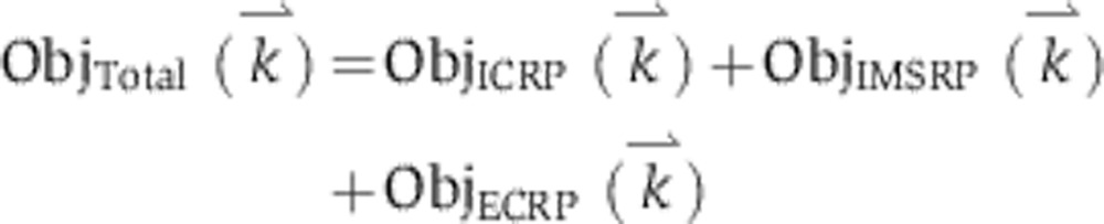
Trajectories for the initiator caspase reporter protein (IC-RP), mitochondrial inter-membrane space reporter protein (IMS-RP), and effector caspase reporter protein (EC-RP) were used from previously published data (Spencer et al, 2009). In the model, tBid, cytosolic Smac, and cleaved PARP were fit to the data for IC-RP, IMS-RP, and EC-RP, respectively. IMS-RP data from 10 cells indicated an average MOMP time of 9810±2690, s after the exposure of the cells to ligand. The IC-RP and EC-RP signals were normalized and aligned to this MOMP time to yield an average trajectory for each. The objective function used to calculate model fit was the sum of component functions for each of the experimental observables as follows:
 |
where  are the rate parameters for the system of
ODEs, and
are the rate parameters for the system of
ODEs, and  ,
,  , and
, and
 are the objective functions for
corresponding observables. These objective functions were defined as
follows:
are the objective functions for
corresponding observables. These objective functions were defined as
follows:
 |
where N=112 is the number of experimental time points,  is the simulated value of tBid at time t (with
the given parameters,
is the simulated value of tBid at time t (with
the given parameters, , Bid0 is the
total amount of Bid in the simulation, and ICRPt is the
distribution of MOMP-aligned experimental IC-RP trajectories at time t.
The objective function for EC-RP was defined similarly, but with cleaved PARP in
place of tBid and EC-RP in place of IC-RP:
, Bid0 is the
total amount of Bid in the simulation, and ICRPt is the
distribution of MOMP-aligned experimental IC-RP trajectories at time t.
The objective function for EC-RP was defined similarly, but with cleaved PARP in
place of tBid and EC-RP in place of IC-RP:
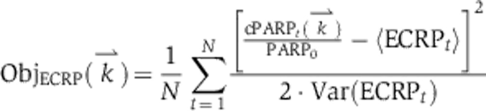 |
Data from previous experiments showed that release of IMS-RP from mitochondria due to MOMP is both rapid and complete under all tested experimental conditions, typically reaching completion within 1–3 min (Albeck et al, 2008a). To ensure that the model could reproduce these kinetics, we used an alternative objective function for the cSmac/IMS-RP signal to consider the onset (TD) and duration (TS) of MOMP:
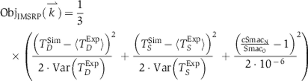 |
 is the experimental ‘death time,’
recorded as the time of MOMP as measured by IMS-RP release;
TSExp is the experimental
‘switching time,’ defined as the time required for IMS-RP to be
released, estimated to have a mean value of 180 s and a variance of 3600,
s2. The corresponding simulated values were defined as
is the experimental ‘death time,’
recorded as the time of MOMP as measured by IMS-RP release;
TSExp is the experimental
‘switching time,’ defined as the time required for IMS-RP to be
released, estimated to have a mean value of 180 s and a variance of 3600,
s2. The corresponding simulated values were defined as
 |
 |
where T90 and T10 are the times taken by the simulation to
reach 90% and 10% of maximum Smac release, respectively. The final
term in  constrains the simulated Smac trajectory
to achieve approximately 100% release: cSmacN is the
final simulated value of cytosolic Smac, and Smac0 is total Smac.
constrains the simulated Smac trajectory
to achieve approximately 100% release: cSmacN is the
final simulated value of cytosolic Smac, and Smac0 is total Smac.
Supplementary Material
Supplementary Figures S1–3
EARM 2.0-M1a in SBML Format
Acknowledgments
We thank A Keating and E Fire for their assistance in the early stages of this project and W Fontana, J Gunawardena, and A Mallavarapu for their help and advice. This work was supported by NIH grants P50-GM68762 and P01- CA139980. CFL was supported by The Harold Whitworth Pierce Charitable Trust (through The Medical Foundation) and NIH Transition to Independence grant K22-CA151918.
Author contributions: CFL, JLM and JAB co-wrote the PySB and EARM 2.0 code, and along with PKS conceived the overall approach and wrote the paper.
Footnotes
The authors declare that they have no conflict of interest.
References
- Albeck JG, Burke JM, Aldridge BB, Zhang M, Lauffenburger DA, Sorger PK (2008a) Quantitative analysis of pathways controlling extrinsic apoptosis in single cells. Mol Cell 30: 11–25 [DOI] [PMC free article] [PubMed] [Google Scholar]
- Albeck JG, Burke JM, Spencer SL, Lauffenburger DA, Sorger PK (2008b) Modeling a snap-action, variable-delay switch controlling extrinsic cell death. PLoS Biol 6: 2831–2852 [DOI] [PMC free article] [PubMed] [Google Scholar]
- Aldridge BB, Gaudet S, Lauffenburger DA, Sorger PK (2011) Lyapunov exponents and phase diagrams reveal multi-factorial control over TRAIL-induced apoptosis. Mol Syst Biol 7: 553. [DOI] [PMC free article] [PubMed] [Google Scholar]
- Bachman JA, Sorger P (2011) New approaches to modeling complex biochemistry. Nat Meth 8: 130–131 [DOI] [PMC free article] [PubMed] [Google Scholar]
- Bagci E, Vodovotz Y, Billiar T, Ermentrout G, Bahar I (2006) Bistability in apoptosis: roles of bax, bcl-2, and mitochondrial permeability transition pores. Biophys J 90: 1546–1559 [DOI] [PMC free article] [PubMed] [Google Scholar]
- Batchelor E, Mock CS, Bhan I, Loewer A, Lahav G (2008) Recurrent initiation: a mechanism for triggering p53 pulses in response to DNA damage. Mol Cell 30: 277–289 [DOI] [PMC free article] [PubMed] [Google Scholar]
- Bentele M, Lavrik I, Ulrich M, Stösser S, Heermann DW, Kalthoff H, Krammer PH, Eils R (2004) Mathematical modeling reveals threshold mechanism in CD95-induced apoptosis. J Cell Biol 166: 839–851 [DOI] [PMC free article] [PubMed] [Google Scholar]
- Billen LP, Kokoski CL, Lovell JF, Leber B, Andrews DW (2008) Bcl-XL inhibits membrane permeabilization by competing with Bax. PLoS Biol 6: e147. [DOI] [PMC free article] [PubMed] [Google Scholar]
- Blinov ML, Faeder JR, Goldstein B, Hlavacek WS (2006) A network model of early events in epidermal growth factor receptor signaling that accounts for combinatorial complexity. BioSystems 83: 136–151 [DOI] [PubMed] [Google Scholar]
- Brown P, Hindmarsh A, Byrne G (1989) VODE: a variable coefficient ODE solver.. SIAM J Sci Stat Comput 10: 1038–1051 [Google Scholar]
- Certo M, Del Gaizo Moore V, Nishino M, Wei G, Korsmeyer S, Armstrong SA, Letai A (2006) Mitochondria primed by death signals determine cellular addiction to antiapoptotic BCL-2 family members. Cancer Cell 9: 351–365 [DOI] [PubMed] [Google Scholar]
- Chen C, Cui J, Lu H, Wang R, Zhang S, Shen P (2007a) Modeling of the role of a Bax-activation switch in the mitochondrial apoptosis decision. Biophys J 92: 4304–4315 [DOI] [PMC free article] [PubMed] [Google Scholar]
- Chen C, Cui J, Zhang W, Shen P (2007b) Robustness analysis identifies the plausible model of the Bcl-2 apoptotic switch. FEBS Lett 581: 5143–5150 [DOI] [PubMed] [Google Scholar]
- Chen L, Willis SN, Wei A, Smith BJ, Fletcher JI, Hinds MG, Colman PM, Day CL, Adams JM, Huang DCS (2005) Differential targeting of prosurvival Bcl-2 proteins by their BH3-only ligands allows complementary apoptotic function. Mol Cell 17: 393–403 [DOI] [PubMed] [Google Scholar]
- Chen WW, Schoeberl B, Jasper PJ, Niepel M, Nielsen UB, Lauffenburger DA, Sorger PK (2009) Input-output behavior of ErbB signaling pathways as revealed by a mass action model trained against dynamic data. Mol Syst Biol 5: 239. [DOI] [PMC free article] [PubMed] [Google Scholar]
- Chylek LA, Hu B, Blinov ML, Emonet T, Faeder JR, Goldstein B, Gutenkunst RN, Haugh JM, Lipniacki T, Posner RG, Yang J, Hlavacek WS (2011) Guidelines for visualizing and annotating rule-based models. Mol Biosyst 7: 2779–2795 [DOI] [PMC free article] [PubMed] [Google Scholar]
- Cui J, Chen C, Lu H, Sun T, Shen P (2008) Two independent positive feedbacks and bistability in the Bcl-2 apoptotic switch. PLoS ONE 3: e1469. [DOI] [PMC free article] [PubMed] [Google Scholar]
- Danos V (2007) Agile modelling of cellular signalling. AIP Conference Proceedings 963: 611–614 [Google Scholar]
- Danos V, Feret J, Fontana W, Harmer R, Krivine J (2007b) Rule-based modelling of cellular signalling. Lect Notes Comput Sci 4703: 17–41 [Google Scholar]
- Danos V, Feret J, Fontana W, Harmer R, Krivine J (2009) Rule-based modelling and model perturbation. Lect Notes Comput Sci 5750: 116–137 [Google Scholar]
- Danos V, Feret J, Fontana W, Krivine J (2007a) Scalable simulation of cellular signaling networks. Lect Notes Comput Sci 4807: 139–157 [Google Scholar]
- Danos V, Feret J, Fontana W, Krivine J (2008) Abstract interpretation of cellular signalling networks. Lect Notes Comput Sci 4905: 83–97 [Google Scholar]
- Debartolo J, Dutta S, Reich L, Keating AE (2012) Predictive bcl-2 family binding models rooted in experiment or structure. J Mol Biol 422: 124–144 [DOI] [PMC free article] [PubMed] [Google Scholar]
- Deeds EJ, Krivine J, Feret J, Danos V, Fontana W (2012) Combinatorial complexity and compositional drift in protein interaction networks. PLoS ONE 7: e32032. [DOI] [PMC free article] [PubMed] [Google Scholar]
- Del Vecchio D, Ninfa AJ, Sontag ED (2008) Modular cell biology: retroactivity and insulation. Mol Syst Biol 4: 161. [DOI] [PMC free article] [PubMed] [Google Scholar]
- Düssmann H, Rehm M, Concannon CG, Anguissola S, Würstle M, Kacmar S, Völler P, Huber HJ, Prehn JHM (2010) Single-cell quantification of Bax activation and mathematical modelling suggest pore formation on minimal mitochondrial Bax accumulation. Cell Death Differ 17: 278–290 [DOI] [PubMed] [Google Scholar]
- Faeder JR, Blinov ML, Hlavacek WS (2009) Rule-based modeling of biochemical systems with BioNetGen. Methods Mol Biol 500: 113–167 [DOI] [PubMed] [Google Scholar]
- Feret J, Danos V, Krivine J, Harmer R, Fontana W (2009) Internal coarse-graining of molecular systems. Proc Natl Acad Sci USA 106: 6453–6458 [DOI] [PMC free article] [PubMed] [Google Scholar]
- Fire E, Gullá SV, Grant RA, Keating AE (2010) Mcl-1-Bim complexes accommodate surprising point mutations via minor structural changes. Prot Sci 19: 507–519 [DOI] [PMC free article] [PubMed] [Google Scholar]
- Fricker N, Beaudouin J, Richter P, Eils R, Krammer PH, Lavrik IN (2010) Model-based dissection of CD95 signaling dynamics reveals both a pro- and antiapoptotic role of c-FLIPL. J Cell Biol 190: 377–389 [DOI] [PMC free article] [PubMed] [Google Scholar]
- Gansner ER, North SC (2000) An open graph visualization system and its applications to software engineering. Software: Practice and Experience 30: 1203–1233 [Google Scholar]
- Gaudet S, Spencer SL, Chen WW, Sorger PK (2012) Exploring the contextual sensitivity of factors that determine cell-to-cell variability in receptor-mediated apoptosis. PLoS Comput Biol 8: e1002482. [DOI] [PMC free article] [PubMed] [Google Scholar]
- Gavathiotis E, Reyna DE, Davis ML, Bird GH, Walensky LD (2010) BH3-triggered structural reorganization drives the activation of proapoptotic BAX. Mol Cell 40: 481–492 [DOI] [PMC free article] [PubMed] [Google Scholar]
- Gnad F, Estrada J, Gunawardena J (2012) Proteus: a web-based, context-specific modelling tool for molecular networks. Bioinformatics 28: 1284–1286 [DOI] [PMC free article] [PubMed] [Google Scholar]
- Goldstein JC, Kluck RM, Green DR (2000) A single cell analysis of apoptosis. Ordering the apoptotic phenotype. Ann N Y Acad Sci 926: 132–141 [DOI] [PubMed] [Google Scholar]
- Hlavacek W, Faeder J, Blinov M, Posner R (2006) Rules for modeling signal-transduction systems. Sci STKE 2006: re6. [DOI] [PubMed] [Google Scholar]
- Hlavacek WS (2009) How to deal with large models? Mol Syst Biol 5: 240. [DOI] [PMC free article] [PubMed] [Google Scholar]
- Hoops S, Sahle S, Gauges R, Lee C, Pahle J, Simus N, Singhal M, Xu L, Mendes P, Kummer U (2006) COPASI—a COmplex PAthway SImulator. Bioinformatics 22: 3067–3074 [DOI] [PubMed] [Google Scholar]
- Howells CC, Baumann WT, Samuels DC, Finkielstein CV (2010) The Bcl-2-associated death promoter (BAD) lowers the threshold at which the Bcl-2-interacting domain death agonist (BID) triggers mitochondria disintegration. J Theor Biol 271: 114–123 [DOI] [PubMed] [Google Scholar]
- Huber HJ, Dussmann H, Kilbride SM, Rehm M, Prehn JHM (2011) Glucose metabolism determines resistance of cancer cells to bioenergetic crisis after cytochrome-c release. Mol Syst Biol 7: 470. [DOI] [PMC free article] [PubMed] [Google Scholar]
- Hucka M, Finney A, Sauro HM, Bolouri H, Doyle JC, Kitano H, Arkin AP, Bornstein BJ, Bray D, Cornish-Bowden A, Cuellar AA, Dronov S, Gilles ED, Ginkel M, Gor V, Goryanin II, Hedley WJ, Hodgman TC, Hofmeyr JH, Hunter PJ et al. (2003) The systems biology markup language (SBML): a medium for representation and exchange of biochemical network models. Bioinformatics 19: 524–531 [DOI] [PubMed] [Google Scholar]
- Hunter JD (2007) Matplotlib: A 2D graphics environment. Comput Sci Eng 9: 90–95 [Google Scholar]
- Kim H, Rafiuddin-Shah M, Tu H-C, Jeffers JR, Zambetti GP, Hsieh JJ-D, Cheng EH-Y (2006) Hierarchical regulation of mitochondrion-dependent apoptosis by BCL-2 subfamilies. Nat Cell Biol 8: 1348–1358 [DOI] [PubMed] [Google Scholar]
- Kim H, Tu H-C, Ren D, Takeuchi O, Jeffers JR, Zambetti GP, Hsieh JJ-D, Cheng EH-Y (2009) Stepwise activation of BAX and BAK by tBID, BIM, and PUMA initiates mitochondrial apoptosis. Mol Cell 36: 487–499 [DOI] [PMC free article] [PubMed] [Google Scholar]
- Kitano H, Funahashi A, Matsuoka Y, Oda K (2005) Using process diagrams for the graphical representation of biological networks. Nat Biotechnol 23: 961–966 [DOI] [PubMed] [Google Scholar]
- Kleiman LB, Maiwald T, Conzelmann H, Lauffenburger DA, Sorger PK (2011) Rapid phospho-turnover by receptor tyrosine kinases impacts downstream signaling and drug binding. Mol Cell 43: 723–737 [DOI] [PMC free article] [PubMed] [Google Scholar]
- Krakauer DC, Collins JP, Erwin D, Flack JC, Fontana W, Laubichler MD, Prohaska SJ, West GB, Stadler PF (2011) The challenges and scope of theoretical biology. J Theor Biol 276: 269–276 [DOI] [PubMed] [Google Scholar]
- Kutumova EO, Kiselev IN, Sharipov RN, Lavrik IN, Kolpakov FA (2012) A modular model of the apoptosis machinery. Adv Exp Med Biol 736: 235–245 [DOI] [PubMed] [Google Scholar]
- Kuwana T, Bouchier-Hayes L, Chipuk JE, Bonzon C, Sullivan BA, Green DR, Newmeyer DD (2005) BH3 domains of BH3-only proteins differentially regulate Bax-mediated mitochondrial membrane permeabilization both directly and indirectly. Mol Cell 17: 525–535 [DOI] [PubMed] [Google Scholar]
- Le Novère N, Finney A, Hucka M, Bhalla US, Campagne F, Collado-Vides J, Crampin EJ, Halstead M, Klipp E, Mendes P, Nielsen P, Sauro H, Shapiro B, Snoep JL, Spence HD, Wanner BL (2005) Minimum information requested in the annotation of biochemical models (MIRIAM). Nat Biotechnol 23: 1509–1515 [DOI] [PubMed] [Google Scholar]
- Leber B, Lin J, Andrews DW (2010) Still embedded together binding to membranes regulates Bcl-2 protein interactions. Oncogene 29: 5221–5230 [DOI] [PMC free article] [PubMed] [Google Scholar]
- Legewie S, Blüthgen N, Herzel H (2006) Mathematical modeling identifies inhibitors of apoptosis as mediators of positive feedback and bistability. PLoS Comput Biol 2: e120. [DOI] [PMC free article] [PubMed] [Google Scholar]
- Letai A, Bassik MC, Walensky LD, Sorcinelli MD, Weiler S, Korsmeyer SJ (2002) Distinct BH3 domains either sensitize or activate mitochondrial apoptosis, serving as prototype cancer therapeutics. Cancer Cell 2: 183–192 [DOI] [PubMed] [Google Scholar]
- Llambi F, Moldoveanu T, Tait SWG, Bouchier-Hayes L, Temirov J, Mccormick LL, Dillon CP, Green DR (2011) A unified model of mammalian BCL-2 protein family interactions at the mitochondria. Mol Cell 44: 517–531 [DOI] [PMC free article] [PubMed] [Google Scholar]
- Lovell JF, Billen LP, Bindner S, Shamas-Din A, Fradin C, Leber B, Andrews DW (2008) Membrane binding by tBid initiates an ordered series of events culminating in membrane permeabilization by Bax. Cell 135: 1074–1084 [DOI] [PubMed] [Google Scholar]
- Maiwald T, Timmer J (2008) Dynamical modeling and multi-experiment fitting with PottersWheel. Bioinformatics 24: 2037–2043 [DOI] [PMC free article] [PubMed] [Google Scholar]
- Mallavarapu A, Thomson M, Ullian B, Gunawardena J (2008) Programming with models: modularity and abstraction provide powerful capabilities for systems biology. J R Soc Interface 6: 257–270 [DOI] [PMC free article] [PubMed] [Google Scholar]
- Martinez-Caballero S, Dejean LM, Kinnally MS, Oh KJ, Mannella CA, Kinnally KW (2009) Assembly of the mitochondrial apoptosis-induced channel, MAC. J Biol Chem 284: 12235–12245 [DOI] [PMC free article] [PubMed] [Google Scholar]
- Mathworks, Inc.. (2012) MATLAB release 2012b The Mathworks, Inc.: Natick, Massachusetts [Google Scholar]
- Mirschel S, Steinmetz K, Rempel M, Ginkel M, Gilles ED (2009) PROMOT: modular modeling for systems biology. Bioinformatics 25: 687–689 [DOI] [PMC free article] [PubMed] [Google Scholar]
- Moraru II, Schaff JC, Slepchenko BM, Loew LM (2002) The virtual cell: an integrated modeling environment for experimental and computational cell biology. Ann N Y Acad Sci 971: 595–596 [DOI] [PubMed] [Google Scholar]
- Muzzey D, Gómez-Uribe CA, Mettetal JT, van Oudenaarden A (2009) A systems-level analysis of perfect adaptation in yeast osmoregulation. Cell 138: 160–171 [DOI] [PMC free article] [PubMed] [Google Scholar]
- Mérino D, Giam M, Hughes PD, Siggs OM, Heger K, O'Reilly LA, Adams JM, Strasser A, Lee EF, Fairlie WD, Bouillet P (2009) The role of BH3-only protein Bim extends beyond inhibiting Bcl-2-like prosurvival proteins. J Cell Biol 186: 355–362 [DOI] [PMC free article] [PubMed] [Google Scholar]
- Neumann L, Pforr C, Beaudouin J, Pappa A, Fricker N, Krammer PH, Lavrik IN, Eils R (2010) Dynamics within the CD95 death-inducing signaling complex decide life and death of cells. Mol Syst Biol 6: 352. [DOI] [PMC free article] [PubMed] [Google Scholar]
- O'Connor CL, Anguissola S, Huber HJ, Dussmann H, Prehn JHM, Rehm M (2008) Intracellular signaling dynamics during apoptosis execution in the presence or absence of X-linked-inhibitor-of-apoptosis-protein. Biochim Biophys Acta 1783: 1903–1913 [DOI] [PubMed] [Google Scholar]
- Oliphant TE (2007) Python for Scientific Computing. Comput. Sci. Eng 9: 10–20 [Google Scholar]
- Pedersen M, Plotkin G (2008) A language for biochemical systems. Lecture Notes in Computer Science 5307: 63–82 [Google Scholar]
- Rehm M, Dussmann H, Janicke RU, Tavare JM, Kogel D, Prehn JHM (2002) Single-cell fluorescence resonance energy transfer analysis demonstrates that caspase activation during apoptosis is a rapid process. Role of caspase-3. J Biol Chem 277: 24506–24514 [DOI] [PubMed] [Google Scholar]
- Rehm M, Huber HJ, Dussmann H, Prehn JHM (2006) Systems analysis of effector caspase activation and its control by X-linked inhibitor of apoptosis protein. EMBO J 25: 4338–4349 [DOI] [PMC free article] [PubMed] [Google Scholar]
- Rehm M, Huber HJ, Hellwig CT, Anguissola S, Dussmann H, Prehn JHM (2009) Dynamics of outer mitochondrial membrane permeabilization during apoptosis. Cell Death Differ 16: 613–623 [DOI] [PubMed] [Google Scholar]
- Ren D, Tu H-C, Kim H, Wang GX, Bean GR, Takeuchi O, Jeffers JR, Zambetti GP, Hsieh JJ-D, Cheng EH-Y (2010) BID, BIM, and PUMA are essential for activation of the BAX- and BAK-dependent cell death program. Science 330: 1390–1393 [DOI] [PMC free article] [PubMed] [Google Scholar]
- Schleich K, Warnken U, Fricker N, Öztürk S, Richter P, Kammerer K, Schnölzer M, Krammer PH, Lavrik IN (2012) Stoichiometry of the CD95 death-inducing signaling complex: experimental and modeling evidence for a death effector domain chain model. Mol Cell 47: 306–319 [DOI] [PubMed] [Google Scholar]
- Smith AM, Xu W, Sun Y, Faeder JR, Marai GE (2012) RuleBender: integrated modeling, simulation and visualization for rule-based intracellular biochemistry. BMC Bioinformatics 13(Suppl 8): S3. [DOI] [PMC free article] [PubMed] [Google Scholar]
- Sneddon MW, Faeder JR, Emonet T (2010) Efficient modeling, simulation and coarse-graining of biological complexity with NFsim. Nat Meth 8: 177–183 [DOI] [PubMed] [Google Scholar]
- Spencer SL, Gaudet S, Albeck JG, Burke JM, Sorger PK (2009) Non-genetic origins of cell-to-cell variability in TRAIL-induced apoptosis. Nature 459: 428–432 [DOI] [PMC free article] [PubMed] [Google Scholar]
- SymPy Development Team. (2012) SymPy: Python library for symbolic mathematics. Available at http://www.sympy.org
- Tan C, Dlugosz PJ, Peng J, Zhang Z, Lapolla SM, Plafker SM, Andrews DW, Lin J (2006) Auto-activation of the apoptosis protein Bax increases mitochondrial membrane permeability and is inhibited by Bcl-2. J Biol Chem 281: 14764–14775 [DOI] [PMC free article] [PubMed] [Google Scholar]
- Tiger C-F, Krause F, Cedersund G, Palmér R, Klipp E, Hohmann S, Kitano H, Krantz M (2012) A framework for mapping, visualisation and automatic model creation of signal-transduction networks. Mol Syst Biol 8: 578. [DOI] [PMC free article] [PubMed] [Google Scholar]
- Waltemath D, Adams R, Bergmann FT, Hucka M, Kolpakov F, Miller AK, Moraru II, Nickerson D, Sahle S, Snoep JL, Le Novère N (2011) Reproducible computational biology experiments with SED-ML-the simulation experiment description markup language. BMC Syst Biol 5: 198. [DOI] [PMC free article] [PubMed] [Google Scholar]
- Willis SN, Chen L, Dewson G, Wei A, Naik E, Fletcher JI, Adams JM, Huang DCS (2005) Proapoptotic Bak is sequestered by Mcl-1 and Bcl-xL, but not Bcl-2, until displaced by BH3-only proteins. Genes Dev 19: 1294–1305 [DOI] [PMC free article] [PubMed] [Google Scholar]
- Willis SN, Fletcher JI, Kaufmann T, van Delft MF, Chen L, Czabotar PE, Ierino H, Lee EF, Fairlie WD, Bouillet P, Strasser A, Kluck RM, Adams JM, Huang DCS (2007) Apoptosis initiated when BH3 ligands engage multiple Bcl-2 homologs, not Bax or Bak. Science 315: 856–859 [DOI] [PubMed] [Google Scholar]
- Wolfram Research, Inc.. (2010) Mathematica 8th edn. Wolfram Research, Inc.: Champaign, Illinois [Google Scholar]
- Xu T-R, Vyshemirsky V, Gormand A, Kriegsheim von A, Girolami M, Baillie GS, Ketley D, Dunlop AJ, Milligan G, Houslay MD, Kolch W (2010) Inferring signaling pathway topologies from multiple perturbation measurements of specific biochemical species. Sci Signal 3: ra20. [PubMed] [Google Scholar]
- Youle RJ, Strasser A (2008) The BCL-2 protein family: opposing activities that mediate cell death. Nat Rev Mol Cell Biol 9: 47–59 [DOI] [PubMed] [Google Scholar]
Associated Data
This section collects any data citations, data availability statements, or supplementary materials included in this article.
Supplementary Materials
Supplementary Figures S1–3
EARM 2.0-M1a in SBML Format