Abstract
A key issue in drug development is to understand the hidden relationships among drugs and targets. Computational methods for novel drug target predictions can greatly reduce time and costs compared with experimental methods. In this paper, we propose a network based computational approach for novel drug and target association predictions. More specifically, a heterogeneous drug-target graph, which incorporates known drug-target interactions as well as drug-drug and target-target similarities, is first constructed. Based on this graph, a novel graph-based inference method is introduced. Compared with two state-of-the-art methods, large-scale cross-validation results indicate that the proposed method can greatly improve novel target predictions.
1. Introduction
Drug targets are a class of molecular structures which could interact with drugs1. Establishing new connections between existing drugs and targets or finding novel targets for a given drug plays an important role in drug development. Experimental prediction of drug-target associations is a laborious and costly task2. So far there are only about a few hundreds of known targets1. In contrast, there are many more computationally predicted targets, e.g., the so called druggable genome3,4. The druggable genome denotes a set of human genes that encode proteins which might be able to bind drug-like molecules3. Though different sets of druggable genes have been predicted, the consensus on the number of druggable genes is around 30004. Due to the large number of potential targets, examining each one of them with a specific drug becomes a tedious or even impossible task. From this point of view, an accurate druggable genome filtering or ranking approach becomes in urgent need.
In recent years, a large number of approaches have been proposed to address this problem. Zhu, et al. (2005)5 attempted to mine implicit chemical compound and gene relations from their co-occurrences in the literature. However, their results were constrained to current knowledge. Furthermore, there are many inconsistencies in target names and drug names, which may adversely affect the accuracy of the results. By using some basic biophysical principles, the structure based maximal affinity model6 could generate accurate predictions of druggability based solely on the crystal structure of a target’s binding site. This method, however, is applicable only when the 3D structures of targets are known, which may not be available in general. More recently, several methods have combined drug-drug or target-target similarities into novel target predictions7–13. Phenotypic side-effect similarities were used to build a drug-drug relation network, based on which novel drug-target associations were inferred7. Yamanishi and coauthors8,9 formalized the drug-target interaction inference as a supervised learning problem on a bipartite graph. The learning process was based on a unified ‘pharmacological space’, which was constructed by combining chemical and genomic properties. It has also been shown that chemical similarities between drugs and ligands, small molecules that bind to molecular targets, can be used to predict unanticipated associations10. Bipartite local models (BLM) used supervised methods to predict target proteins of a given drug, then to predict drugs targeting a given protein, and finally these two steps were combined to give a final prediction for each drug-target interaction11. In another work, Perlman et al. (2011)12 proposed a framework that combines multiple drug-drug and gene-gene similarity measures using a logistic regression model. The final classification score was used to indicate interactions between drugs and targets. Very recently, a network based inference (NBI) method was proposed to infer novel drug-target interactions13, which ranks drugs for a specific target based on a two-step diffusion model on the bipartite drug-target graph.
The guilt-by-association principle has been widely used in many different domains and applications (e.g., Jeh and Widom (2002)14). Chiang and Butte (2009)15 proposed a novel drug repositioning method based on the guilt-by-association principle. They claimed that suggestions for novel drug uses can be generated from the uses of drugs that cure the same diseases. This assumption was further extended by concluding that similar diseases tend to be connected with similar drugs and similar drugs tend to be connected with similar target16. Based on this assumption, the intra-similarity information can be incorporated into novel association predictions by constructing a heterogeneous drug-target graph/network, which includes both intra-similarity information (connections between the same kind of nodes, such as drug-drug connections and target-target connections) and interaction information (connections between different kinds of nodes, such as drug-target connections). In this paper, we propose a method, termed HGBI, for Heterogeneous Graph Based Inference, for novel drug target predictions based on the guilt-by-association principle and an intuitive interpretation of information flow on the drug-target heterogeneous graph. The algorithm iteratively updates the measure of strength between unlinked drug-target pairs based on all the paths in the network connecting them. We show that when properly normalized, the proposed procedure will eventually converge and stable relationships between drugs and targets can be achieved. Fig. 1 shows the framework of HGBI. Based on large scale leave-one-out cross-validation experiments, we show that HGBI exhibited superior performance and achieved much higher AUC (area under the receiver operating characteristic, i.e., ROC curve) than two existing state-of-the-art novel drug target prediction methods, BLM11 and NBI13. In particularly, when focusing on the top 1% ranked targets, HGBI successfully retrieved 1339 out of 1915 drug-target interactions, whereas BLM and NBI only retrieved 56 and 10 such interactions. Furthermore, HGBI can establish a novel interaction between a drug and a target even none of the two have directly associated targets/drugs. Some of these novel predictions are confirmed based on a new database, which is not used in this study.
Fig. 1.
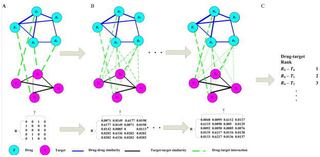
The framework of HGBI. A: A heterogeneous graph is constructed based on drug-drug similarities, target-target similarities, and drug-target interactions. B: Edge weights between drugs and targets are updated iteratively by incorporating all possible paths between each drug-target pair. C: For each drug, all candidate targets are ranked according to the final weights.
2. Materials and methods
2.1 Datasets collection
There are two intra-similarity matrices which represent the drug-drug similarities and target-target similarities, respectively. In addition, there is an interaction matrix, i.e. the drug-target interaction matrix, which represents the connections between drugs and targets. The drug-drug similarity matrix includes all the FDA-approved drugs from the DrugBank database17. The similarities are calculated based on their chemical structures. First, chemical structures of all drug compounds in the Canonical SMILES format18 are downloaded from DrugBank17. Then, the Chemical Development Kit19 is used to calculate a binary fingerprint for each drug. Finally, a similarity score of two drugs is calculated using Tanimoto score20 based on their fingerprints, which is in the range of [0, 1]. A druggable gene is defined as a human protein coding gene that contributes to a disease phenotype and can be modified by a small molecule drug. The term “druggable genome” has been used to denote a list of computationally predicted genes that their proteins can serve as suitable targets for developing therapeutic drugs21. We use the term “druggable gene” and “target” interchangeably in this study. The list of druggable genes is downloaded from the Sophic Integrated Druggable Genome Database project21, which includes genes from the ENSEMBL database22, the DrugBank database17 and the InterPro-BLAST database23. The target-target similarities are calculated using the Smith-Waterman algorithm24 based on the amino acid sequences of their corresponding proteins. The similarities are normalized using the same method proposed by Bleakley and Yamanishi (2009)11. Initial drug-target interactions are collected from the DrugBank database17, but limited to drugs that have associated diseases in the Online Mendelian Inheritance in Man (OMIM) database25, which are the same as the one used in Ref16. For each drug-target interaction, their corresponding value in the drug-target interaction matrix is 1. All other items in the drug-target matrix are set to 0.
2.2 Basic statistics
The total number of drugs is 1409. The total number of targets is 3997. The matrix is very sparse with many isolated nodes (having no connections). The total number of connections among drugs and targets is only 2098, with 554 drugs having at least one known target and 602 targets connecting with at least one drug. Among the connected nodes, many of them have more than one connection, which means known information about drugs and targets is biased towards a very small subset of all drugs/targets. The degree distribution of each entity in the matrix is given in Fig. 2.
Fig. 2.
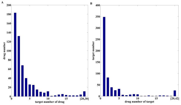
Degree distributions of drugs (A) and targets (B) among the initial drug-target interactions.
2.3 Intra-similarity analysis
Before performing the proposed approach, we first study the statistical characteristics of these datasets. The distributions of the two intra-similarity matrices, i.e. the drug-drug and the target-target similarity matrices, are presented in Fig. 3A&C, which show the majority of the similarities are quite small. According to previous studies26,27, low level similarity values provide little information for interaction inference. Furthermore, including the mess of low values could adversely affect prediction performance. Therefore, for the constructed heterogeneous graph, two nodes of the same type are connected only if their similarity score ≥ 0.3. It is also noted that although the entries between a node to itself have already been excluded, there are still some entries with value 1 (Fig. 3B&D), which is mainly due to the representation issue. To ensure that a node can only have a similarity score of 1 to itself, we replace those 1s with 0.99, which should not affect the final results much.
Fig. 3.
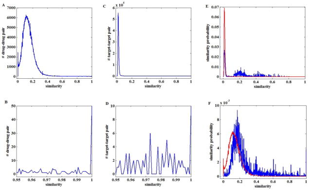
Intra-similarity distributions. A: the distribution of drug-drug similarities; B: the tail distribution of drug-drug similarities in the range of (0.95, 1); C: the distribution of target-target similarities; D: the tail distribution of target-target similarities in the range of (0.95, 1); E: similarity distributions of targets sharing the same drugs (blue curve), and from different drugs (red curve); F: similarity distributions of drugs sharing the same targets (blue curve), and from different targets (red curve).
This study is based on the assumption that similar drugs tend to be associated with similar targets and dissimilar drugs are prone to be associated with dissimilar targets. To study the validation of the assumption on the collected real datasets, similarities of drugs for the same targets and similarities of drugs from different targets are compared. The average similarity of drugs for the same targets is calculated by averaging the similarities of all drug pairs that belong to the same target. To determine the average similarity of drugs from different targets, the similarity values of all drug pairs that are across different targets are averaged. Similarly, we examine the similarities among targets that share the same drugs and similarities among targets that do not share any drugs. The results are given in Fig. 3E&F. The average similarity of drug pairs from the same targets and the average similarity of target pairs from the same drugs are 0.2445 and 0.1836, respectively. In contrast, the average similarity of drug pairs from different targets and the average similarity of target pairs from different drugs are 0.1429 and 0.0231, respectively. We further test the differences of the corresponding distributions using the Wilcoxon rank sum test. Both tests reject the null hypothesis that the distributions are the same at the 5% significance level. Based on these results, it can be concluded that drugs (targets) associated with the same targets (drugs) possess higher similarity values than those associated with different targets (drugs). The guilt-by-association principle can be utilized in this study.
2.4 Drug-target association predictions
The drug-target heterogeneous graph has two kinds of nodes: drug nodes and target nodes. Let R = {R1, R2, …, Rn} denote the n drug nodes, and T = {T1,T2,…,Tm} denote the m target nodes. A drug is connected with another drug if and only if their similarity is greater than a pre-defined threshold (0.3 in this study), which is assigned as the weight of the edge. Edges and weights for target pairs are constructed similarly. Finally, a drug and a target are connected if they interact in the original drug-target interaction dataset. The weights of all drug-target edges are originally assigned 1. Let Err, Ett, and Ert represent drug-drug, target-target and drug-target edges, respectively, and Wrr, Wtt, and Wrt represent the weights on these three kinds of edges. The heterogeneous drug-target graph can be represented as GRT = {{R,T},{Err, Ett, Ert,},{Wrr,Wtt,Wrt,}}. Based on this graph, the novel target prediction problem can be transformed into a novel drug-target edge prediction problem on the constructed drug-target graph. This means that the original heterogeneous graph GRT can be considered as an incomplete graph with missing edges between R (drug) nodes and T (target) nodes. The objective is to capture hidden interactions between drugs and targets based on the drug-drug similarities, target-target similarities, and known drug-target interactions. The novel drug-target edge prediction problem can be formalized as follows:
Input: GRT = {{R,T},{Err, Ett, Ert,},{Wrr,Wtt,Wrt,}}
Output:
where and represent the newly calculated edges and their weights respectively.
Based on the guilt-by-association assumption, the intra-similarities and drug-target associations can be combined together to predict novel interactions between drugs and targets. For example, given the graph GRT, one way to calculate the association coefficient (i.e., weight) between each initially unconnected drug-target pair is based on the following equation,
| (1) |
Here r is a drug and t is a target and they are not connected in the original graph. ri’s and tj’s are the neighbors of r and t that are connected with each other in GRT. w(r,ri) is the weight between r and ri, and w(t,tj) is the weight between t and tj. Equation 1 basically means that one can establish a new weight between a drug and a target by summarizing all paths of length three, consisting one edge in each of Err, Ert, Ett. This is essentially the same idea adopted by NBI13.
Naturally, once new relationships/weights between drugs and targets being established based on equation 1, they themselves can be utilized again to generate more relationships. An iterative procedure can be constructed, which can be represented as matrix multiplications: . In general, there are two related issues that need to be resolved in order to make the proposed iterative approach to work. First, one may want to treat the initial links between drugs and targets differently from the inferred links because the initial links deserve more credibility. Second, it is desirable if the matrix Wrt will converge, which means that the information propagation is stabilized at the end. In this study, we propose an iterative approach based on equation 2, which naturally solves the first problem based on its formulation. Furthermore, we show that with proper normalization, it also solves the second problem.
| (2) |
In this formula, , represents the initial interactions between drugs and targets, α is a decay factor with its value between 0 and 1. In each iteration, the original drug-target interactions will contribute to the newly constructed interactions, and the contribution is controlled by the scale factor 1 − α. Theoretically, one can optimize α based on results from cross validations. In this study, we fix α = 0.4. By iteratively using this formula, the strength between a drug and a target will eventually include all the possible paths connecting them in the heterogeneous graph. We prove that when Wrr and Wtt are properly normalized, it is guaranteed that equation 2 will converge. The result is summarized as Theorem 1 and the details of the proof can be found in the appendix. To obtain the final solution based on equation 2, we use an iterative propagation-based algorithm28. Once the final result is given, for each drug, all the targets will be ranked according to the strength of their links to the drug.
THEOREM 1
When Wrr and Wtt are properly normalized utilizing equation 3, it is guaranteed that formula (2) will converge.
| (3) |
3 Experiments
3.1 Evaluation metrics
In order to systematically evaluate the proposed approach on the collected datasets, we adopt a leave-one-out cross-validation (LOOCV) strategy in our experiments. For each drug, one of its connections to a target is treated as the test data, and it is ranked with all other targets in descending order according to the calculated drug-target association coefficients using the remaining connections as training data. For each specific ranking threshold, if the rank of the testing connection is above the threshold, it is regarded as a true positive. On the other hand, if the rank of an unknown connection is above the threshold, it is regarded as a false positive. True positive rate (TPR) and false positive rate (FPR) are calculated by varying thresholds to construct the ROC curve29. The area under the curve (AUC) value represents the overall performance of the algorithm. In addition to LOOCV, we also perform 10-fold cross-validation, where all the drug-target connections are randomly partitioned into 10 subsets and each subset is treated as the test set in each iteration. Furthermore, in practice, it is natural that most researchers only focus on top ranked targets. Therefore, we also examine the performance of the algorithm on the top ranked results, i.e., the number of correctly retrieved connections based on various top percentiles (the most left side of the ROC curve). In addition, to test the capacity of the algorithm in detecting novel interactions for drugs with no known targets, we collect all drugs that only have a single known target and perform the experiment by removing the only interaction. Finally, using all the data as training data, we test our algorithm again and compare the top ranked targets with those in another database 30 that is not used in training.
3.2 Comparison with existing methods
To evaluate the proposed approach, we choose to compare its performance with BLM11 and NBI13. BLM is considered one of the state-of-the-art approaches in drug-target interaction predictions. In this study, BLM is implemented the same way as the one in the original paper11. The predicted scores generated from SVM are used as the ranking criterion, which means that larger predicted scores yield higher ranks. In order to choose a proper number of negative samples for SVM training of BLM, we perform cross-validation. Based on the results (Fig S1 in appendix), the number of negative training samples was set to be max{20, 2 × num_positive_samples}. The result of BLM is obtained by averaging five runs with the same configuration but different negative training samples. We choose to compare with NBI13 because it can be viewed as a simplified version of the proposed approach, in the sense that only a two-step diffusion of the matrices (similar to equation 1) is used in NBI, while our approach uses the converged matrix. NBI13 is implemented according to the original paper.
3.3 Experimental results
3.3.1 Predictions for drugs with known connected targets
The cross-validation experiments for target predictions were conducted using all drugs with at least two known targets. In total, 371 such drugs and 1915 initial drug-target edges were considered. The ROC curves and AUC values of NBI, BLM, HGBI (LOOCV and 10-fold) are given in Fig. 4A. It shows that HGBI (AUC:0.93) significantly outperforms both BLM (AUC:0.89) and NBI (AUC:0.73) for LOOCV. Furthermore, HGBI almost has the same performance when using 10-fold cross-validation. The numbers of correctly retrieved drug-target interactions according to different ranking thresholds are also given in Fig. 4B. Results show that when focusing on the top ranked results, the performance of HGBI is much better compared with NBI and BLM, especially for the top 1% ranked targets, in which case HGBI correctly retrieved 1339 drug-target interactions, whereas BLM and NBI only retrieved 56 and 10 such interactions.
Fig. 4.
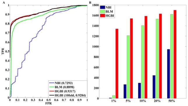
A: ROC curves of drug-target association predictions. AUC of each curve is indicated in the parentheses; B: The number of retrieved drug-target interactions using different thresholds. x-axis is the ranking thresholds in percentile.
3.3.2 Predictions for drugs without known connected targets
To demonstrate the effectiveness of the proposed approach in detecting novel targets for drugs without known targets, only drugs with exactly one connected target in the dataset were collected in this experiment. There are in total 183 such drugs. Because BLM cannot predict novel targets for drugs without known targets, we only compare HGBI with NBI here. The ROC curves of NBI and HGBI are given in Figure 5. Again, HGBI (AUC:0.93) achieves much better performance than NBI (AUC:0.72).
Fig. 5.
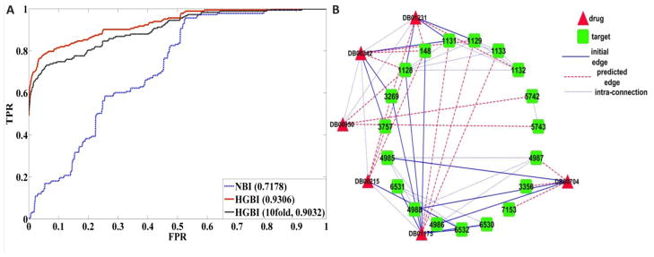
A. ROC curves of novel target predictions for drugs without known targets. B. The subsetwork for the case study.
3.3.3 Case studies on drug -target association predictions
Finally, using all the data as the training data, HBGI can make new predictions for all the drugs in the database. To further analyze its performance for practical usage, six drugs, i.e. Citalopram (Drugbank ID: DB00215), Escitalopram (DB01175), Terfenadine (DB00342), Diphenidol (DB01231), Fexofenadine (DB00950), and Naltrexone (DB00704), were randomly chosen for the case studies. For each drug, all their initial targets and the top 10 predicted targets were collected. A subset of these drugs, targets, and their connections are also illustrated in Fig 5B, which only shows up to 3 known targets and the top 3 predicted targets for clarity. Several observations can be made based on Fig 5B. First, similar drugs tend to share similar predicted targets, such as the drugs Diphenidol and Terfenadine. Second, predictions for drugs without known connected targets, such as the drug Fexofenadine, can be performed using HBGI. Because it is connected with the drug Diphenidol, one of Diphenidol’s targets (target Entrez_ID: 1128 in Fig 5B) is predicted to be associated with it.
We further searched the Supertarget database30, which is an extensive web resource for analyzing drug-target interactions. Some of the top ranked predictions by HBGI are supported by newly reported discoveries in the database. For example, in the Supertarget database, Citalopram (DB00215) has two new targets SLC6A3 (6531) and SLC6A2 (6530) that were not in the DrugBank database. They were ranked as the 2nd and the 17th among all target candidates by HBGI. Similarly, ADRA1D (146) & CHRM1 (1128) were not associated with Terfenadine (DB00342) in the DrugBank database. They were ranked as the 3rd & the 8th, respectively.
In a very recent study31, the authors experimentally validated 123 unique drug-target relationships. In comparison of our prediction with these newly validated relationships, our median rank for this data set is 16 (out of 3997 targets) and 43 of them are ranked in top 10.
4 Conclusion
In this paper, we have proposed a drug target prediction approach, HGBI, which integrates drug-drug similarities, target-target similarities and drug-target interactions into a heterogeneous graph and models the drug-target interactions as the stabilized information flow between them across the heterogeneous graph. Experiments have shown that HGBI significantly outperforms two existing methods in predicting novel targets for drugs with and without known targets. A case study has illustrated that HGBI can be used in practice to rank candidate targets for drugs and many top ranked ones can be utilized for further investigations.
Although equation 2 is similar to the framework of random walk with restart (RWWR)32, it is different in the sense that 1) equation 2 is defined on a heterogeneous graph and only connections between nodes of different types need to be derived; 2) because of the heterogeneous graph, all the information on similar drugs, similar targets and drug-target interactions has been used in predicting new drug-target associations.
For future directions, first, instead of using top ranked targets, it is possible to adopt an automatic threshold to declare significant predictions using the same idea in Ref33. Furthermore, many approaches have been developed to identify disease genes. However, the relationships between disesae genes and drug targets are not totally characterised. It would be interesting to include disease gene information in drug target predictions.
Supplementary Material
Acknowledgments
This research is supported by an NIH/NLM grant (LM008991).
6. Appendix
PROOF of Theorem 1
To make the proof process clear, Let A, B and X denote Wrr, Wtt, and Wrt respectively. A, B and X are n×n, m×m and n×m matrices respectively. Ai and Aj denote the i-th row of A and j-th column of A respectively. aij is used to represent the value at the i-th row and j-th column of matrix A. These conventions are also used for matrix B and X.
Then according to equation (2), we have . For X1, we can also get
If we use Ai × Bj to denote , then equation (2) can be written as
| (4) |
Let C denote and i = sn + t, j = rn + θ, s = sI{t > 0}+ (s − 1)I{t = 0}, t = tI{t > 0}+ nI{t = 0}, r = rI{θ > 0}+ (r − 1)I{θ = 0}, θ = θI{θ > 0}+ nI{θ = 0}, 0 ≤ t, θ < n.
Then we get: ci,j = at,θbr+1,s+1 and cj,i = aθ,t bs+1,r+1
By comparing the above two equations, we can easily find that C is a symmetrical matrix with row and column number n×m. If we use X* to represents , then equation (4) can also be written as:
| (5) |
According to (Vanunu, et al. 2010)29, in order to get a converged solution for equation (5), C is normalized as: Cnorm = D−1/2CD−1/2, where D is diagonal matrix with di,i equals to the sum of the i-th row of C. Therefore, we also have and where u = run + θu. By incorporating the above equation into , we can get
Therefore, if we normalize A and B as and
We can get .
With this equation, we can rewrite equation (5) as X* = αCnormX*+(1−α)X*0
Contributor Information
Wenhui Wang, Email: wxw134@case.edu.
Sen Yang, Email: sxy221@case.edu.
JING Li, Email: jingli@case.edu.
References
- 1.Imming P, et al. Nat Rev Drug Discov. 2006;10:821. doi: 10.1038/nrd2132. [DOI] [PubMed] [Google Scholar]
- 2.Haggarty S, et al. Chem Biol. 2003;5:383. doi: 10.1016/s1074-5521(03)00095-4. [DOI] [PubMed] [Google Scholar]
- 3.Hopkins A, Groom C. Nat Rev Drug Discov. 2002;9:727. doi: 10.1038/nrd892. [DOI] [PubMed] [Google Scholar]
- 4.Russ A, Lampel S. Drug Discov Today. 2005;23–24:1607. doi: 10.1016/S1359-6446(05)03666-4. [DOI] [PubMed] [Google Scholar]
- 5.Zhu S, et al. Bioinformatics. 2005;suppl 2:ii245. doi: 10.1093/bioinformatics/bti1141. [DOI] [PubMed] [Google Scholar]
- 6.Cheng A, et al. Nat Biotechnol. 2007;1:71. doi: 10.1038/nbt1273. [DOI] [PubMed] [Google Scholar]
- 7.Campillos M, et al. Science. 2008;5886:263. doi: 10.1126/science.1158140. [DOI] [PubMed] [Google Scholar]
- 8.Yamanishi Y, Araki M, et al. Bioinformatics. 2008;13:i232. doi: 10.1093/bioinformatics/btn162. [DOI] [PMC free article] [PubMed] [Google Scholar]
- 9.Yamanishi Y. Proceedings of NIPS. 2008;21:1433. [Google Scholar]
- 10.Keiser M, et al. Nature. 2009;7270:175. doi: 10.1038/nature08506. [DOI] [PMC free article] [PubMed] [Google Scholar]
- 11.Bleakley K, Yamanishi Y. Bioinformatics. 2009;18:2397. doi: 10.1093/bioinformatics/btp433. [DOI] [PMC free article] [PubMed] [Google Scholar]
- 12.Perlman L, et al. J Comput Bio. 2011;2:133. doi: 10.1089/cmb.2010.0213. [DOI] [PubMed] [Google Scholar]
- 13.Cheng F, et al. PLoS Comput Biol. 2012;5:e1002503. doi: 10.1371/journal.pcbi.1002503. [DOI] [PMC free article] [PubMed] [Google Scholar]
- 14.Jeh G, Widom J. KDD. 2002;538 [Google Scholar]
- 15.Chiang A, Butte A. Clin Pharmacol Ther. 2009;5:507. doi: 10.1038/clpt.2009.103. [DOI] [PMC free article] [PubMed] [Google Scholar]
- 16.Gottlieb A, et al. Mol Syst Biol. 2011;496:496. doi: 10.1038/msb.2011.26. [DOI] [PMC free article] [PubMed] [Google Scholar]
- 17.Knox C, et al. Nucleic Acids Res. Database issue. 2011;1035 doi: 10.1093/nar/gkq1126. [DOI] [PMC free article] [PubMed] [Google Scholar]
- 18.Weininger D. Journal of Chemical Information and Modeling. 1988;1:31. [Google Scholar]
- 19.Steinbeck C, et al. Curr Pharm Des. 2006;17:2111. doi: 10.2174/138161206777585274. [DOI] [PubMed] [Google Scholar]
- 20.Tanimoto T. IBM Internal Report 17th Nov. 1957. [Google Scholar]
- 21.Sophic. 2012 http://www.sophicalliance.com/documents/sophicdocs/White%20Paper%20Update%201-27-11/The%20Druggable%20Genome012511.pdf.
- 22.Flicek P, et al. Nucleic Acids Res. 2011;800 Database issue. [Google Scholar]
- 23.Hunter S, et al. Nucleic Acids Res. 2009;211 Database issue. [Google Scholar]
- 24.Smith T, Waterman M. J Mol Biol. 1981;1:195. doi: 10.1016/0022-2836(81)90087-5. [DOI] [PubMed] [Google Scholar]
- 25.Hamosh A, et al. Nucleic Acids Res. 2002;30:52. doi: 10.1093/nar/30.1.52. [DOI] [PMC free article] [PubMed] [Google Scholar]
- 26.Chen Y, et al. Bioinformatics. 2011;13:i167. doi: 10.1093/bioinformatics/btr213. [DOI] [PMC free article] [PubMed] [Google Scholar]
- 27.van Driel M, et al. Eur J Hum Genet. 2006;5:535. doi: 10.1038/sj.ejhg.5201585. [DOI] [PubMed] [Google Scholar]
- 28.Oron V, et al. PLoS Comput Biol. 2010;1:e1000641. doi: 10.1371/journal.pcbi.1000641. [DOI] [PMC free article] [PubMed] [Google Scholar]
- 29.Sing T, et al. Bioinformatics. 2005;20:3940. doi: 10.1093/bioinformatics/bti623. [DOI] [PubMed] [Google Scholar]
- 30.Hecker N, et al. Nucleic Acids Res. 2012;D1113 doi: 10.1093/nar/gkr912. Database issue. [DOI] [PMC free article] [PubMed] [Google Scholar]
- 31.Lounkine E, et al. Nature. 2012;486:361. doi: 10.1038/nature11159. [DOI] [PMC free article] [PubMed] [Google Scholar]
- 32.Tong, et al. Proceedings of ICDM. 2005:613–622. [Google Scholar]
- 33.Chen, et al. PLoS One. 2011;6:e21137. doi: 10.1371/journal.pone.0021137. [DOI] [PMC free article] [PubMed] [Google Scholar]
Associated Data
This section collects any data citations, data availability statements, or supplementary materials included in this article.


