Model-free forecasting outperforms the correct mechanistic model for simulated and experimental data

Abstract

Accurate predictions of species abundance remain one of the most vexing challenges in ecology. This observation is perhaps unsurprising, because population dynamics are often strongly forced and highly nonlinear. Recently, however, numerous statistical techniques have been proposed for fitting highly parameterized mechanistic models to complex time series, potentially providing the machinery necessary for generating useful predictions. Alternatively, there is a wide variety of comparatively simple model-free forecasting methods that could be used to predict abundance. Here we pose a rather conservative challenge and ask whether a correctly specified mechanistic model, fit with commonly used statistical techniques, can provide better forecasts than simple model-free methods for ecological systems with noisy nonlinear dynamics. Using four different control models and seven experimental time series of flour beetles, we found that Markov chain Monte Carlo procedures for fitting mechanistic models often converged on best-fit parameterizations far different from the known parameters. As a result, the correctly specified models provided inaccurate forecasts and incorrect inferences. In contrast, a model-free method based on state-space reconstruction gave the most accurate short-term forecasts, even while using only a single time series from the multivariate system. Considering the recent push for ecosystem-based management and the increasing call for ecological predictions, our results suggest that a flexible model-free approach may be the most promising way forward.

Understanding fluctuations in species abundance is a long-standing goal of ecology and is particularly important for the conservation of severely depleted populations (1, 2). Dramatic changes in species abundance are common (3) and large declines can have disastrous impacts on ecosystem users (4). Accurate forecasts could allow for improved conservation efforts and increased fishery yields, however, ecological surprises are common (5), and accurate predictions remain a major challenge (6).

As ecological time series continue to lengthen, and computer-intensive statistics become more convenient, there has been an increasing trend toward fitting complex mechanistic models that incorporate both process and observation error (i.e., state-space models) (7). A Bayesian fitting procedure for such a model typically involves computationally intensive Markov chain Monte Carlo (MCMC) sampling of the joint posterior probability distribution to find the best fitting parameters (8). Previous work concluded that misspecified mechanistic models can produce poor forecasts (9), but it has been suggested that state-space models may be more robust to misspecification due to their inclusion of a process-error term (8); however, their forecast accuracy remains largely untested.

Model-free time series analysis provides an alternative method for generating forecasts that, unlike most state-space fitting procedures, does not require intensive computations. Although there exists a vast literature on time series forecasting methods, we focus on three commonly used models: the linear autoregressive (AR) and autoregressive moving average (ARMA) models, and the nonlinear state-space reconstruction (SSR) method. AR and ARMA time series models have been used extensively in ecology; recent examples include forecasting quasi-extinction risk (10), investigating the effects of climate change on fisheries (11), and detecting critical thresholds in ecosystem dynamics (12). SSR methods have been less pervasive in ecology (13, 14), although they are ubiquitous in many other scientific disciplines for describing stochastic nonlinear systems (15).

Here, we pose a rather conservative challenge and ask whether a correctly specified mechanistic model, fit with commonly used statistical techniques, can provide better forecasts than simple model-free methods for ecological systems with noisy nonlinear dynamics. To answer this question, we used computer simulations and experimental data to fit a suite of mechanistic models using a Bayesian MCMC algorithm under ecologically realistic levels of noise. Surprisingly, we found that even using only a single time series variable for each system, an SSR forecast approach consistently outperformed both the linear time series models and the correctly specified mechanistic models.

Simulation Methods

Using four different mechanistic control models, we generated simulated time series with both process noise and observation error (see Table 1 for models and parameters). Each model was fit to a 50-y time series (referred to as the training set) and forecast accuracy was evaluated using an additional 50-y time series that contained no observation error (referred to as the test set). Because each time series contains a unique sequence of process noise, we simulated 100 replicates for each model to ensure robust results. To facilitate comparison of forecast accuracy between models, forecast error is described using the standardized rms error statistic (SRMSE), which is defined as the rms error divided by the SD of the test set. Forecast errors greater than unity indicate predictions less accurate than simply predicting the mean of the test set.

Table 1.

Model structure and model parameter values used in the simulations

Model name	Process model structure*
Logistic
Two-species
Age-structured	x0,t = (x2,t + x3,t)f
	x1,t+1 = x0,texp(r − rx0,t + ɛt)
	x2,t+1 = s1x1,t
	x3,t+1 = s2(x2,t + x3,t)
Spatial

*Process noise ɛ_t is normally distributed with μ = 0 and σ = 0.005.

All species (or age classes) in each model were forecasted. Importantly, however, to make the results more conservative, the model-free methods used only the single time series of the focal species (or age class) to make forecasts, whereas the mechanistic models were fit to the entire multivariate set of time series. In real systems we often lack time series of important driving variables or species; thus, for this additional reason, this comparison represents a very optimistic scenario for the mechanistic modeling approach.

Control Models.

We chose four control models that encompass a wide range of ecological scenarios—the logistic model, a two-species coupled logistic model (16), an age-structured model (17), and a four-patch spatial model (18). Deterministic model structures are given in Table 1 (parameter values given in Table S1).

All control models included log-normal process and observation error, and parameter values that resulted in chaotic or near-chaotic deterministic dynamics. A coefficient of variation (CV) of 0.2 was chosen for the observation error, which is consistent with that reported in fish abundance surveys (19).

To avoid nonidentifiability of error sources, the process noise variance was fixed to the correct value (giving the mechanistic approach yet another advantage), and only the observation error variance was fit. Each control model was fit to its training set using Bayesian adaptive MCMC with Geyer’s algorithm (20) in MATLAB (21) (Table S2); similar results were obtained using R and JAGS (22, 23) (Figs. S1 and S2). All priors were independent, noninformative, truncated-normal distributions with mean equal to the correct parameter value. Convergence of the algorithm was evaluated using the Gelman–Rubin statistic () (24) and batch-mean normal–normal plots (Fig. S3). The Bayesian MCMC fitting method used here is among the most commonly used in ecology (25).

The expected value of the stochastic models closely matched that of their deterministic skeleton (Fig. S4); therefore, forecasts were made using the deterministic model with parameter values corresponding to the mode of the posterior distribution (similar results are obtained using the median). We initiated the MCMC search on the known parameters because likelihood surfaces of chaotic and near-chaotic time series are notoriously rugose (26), and we wanted to ensure that the known model parameters were evaluated; this is a luxury we lack when fitting models to real time series (and represents another advantage given to the approach). Also, in real systems, the control model is never known. Thus, the use of the control model here must be considered a best-case scenario for the mechanistic modeling approach and should be the ultimate advantage in this competition among models.

SSR Time Series Model.

The SSR time series model use Takens’ theorem, which allows for the representation of a multivariate dynamical system through the method of time-delay embedding (27). Takens’ theorem provides the conditions under which a multivariate dynamical system may be reconstructed from a univariate time series by transforming the univariate time series into a set of time-delayed vectors: X_t = [x_t, x_t−τ, x_t−2τ,…, x_{t−(E−1)τ}], where x is the univariate time series, t is the time index, τ is the time lag, and E is the embedding dimension. Provided that E is sufficiently large, the collection of vectors X_t, for t = [1 + (E − 1)τ, …, N], is an embedding of the attracting manifold, where N is the length of the time series.

After transforming the time series into an embedding, we generated predictions using the S-Map model (13, 28, 29), which is a locally weighted autoregressive model of the embedded time series with weights given by

where θ ≥ 0, d is the Euclidean distance between the predictee and the neighbor vector in embedded space, and is the average distance between the predictee and all other vectors. The degree of local weighting (θ) and the embedding dimension (E) were fit using cross-validation on the 50-y training set. We searched to a maximum of E = 9 lags, because the highest dimensionality of the models was n = 4, and it has been shown that any nonlinear stochastic model can be represented by a univariate model of order 2n + 1, where n is the dimension of the true model (30). Predictions were made on the 50-y test set.

Linear Time Series Models.

Last, we evaluated the forecast accuracy of two linear time series models: AR and ARMA. Linear time series models have be used extensively in ecology. The ARMA(p,q) model is given as (31)

where p is the dimension of the autoregressive term, q is the dimension of the moving average term, μ is the mean of the time series, α and β are the coefficients of the autoregressive and moving average terms, respectively, and ε is a normally distributed random variable with mean zero.

It has been shown that many stochastic nonlinear processes, and especially low-order limit cycles, are well approximated by an ARMA model (31); however, the forecast accuracy of such models under large observation error and strong nonlinear dynamics (e.g., chaos) remains largely untested.

Analogous to the nonlinear model, the dimension of the AR and ARMA models was chosen using leave-one-out cross-validation on the 50-y training set, where the maximum dimension tested was 2n + 1 (i.e., the maximum possible value of p and q was 2n + 1). To differentiate between the performance of the AR and ARMA models, we only considered ARMA models that included a moving average component (i.e., parameter q was always greater than zero).

Simulation Results

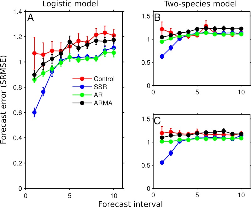
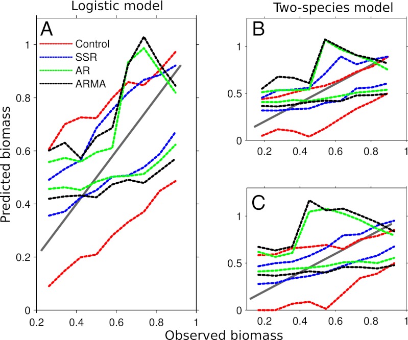
Surprisingly, the SSR time series method consistently provided more accurate short-term forecasts than even the control models. In contrast, the linear forecasting methods were often no better than a prediction of the mean of the test set (represented by SRMSE = 1; Figs. 1 and 2). The performance of the control model varied depending on the system, but it too was often no better than a mean predictor.

Fig. 1.

Forecast error for each forecasting method for the logistic (A) and two-species (B and C) models. Forecast interval is the number of steps ahead for which the prediction is being made. Forecast error (SRMSE) is the rms error of the predictions divided by the SD of the test set. Points represent the mean SRMSE over the 100 simulations for each model; bars are the SE. The red, blue, green, and black lines show the forecast error for the fitted control model, SSR model, AR model, and ARMA model, respectively.

Fig. 2.

Predicted vs. observed for the logistic (A) and two-species models (species x and y are B and C, respectively). One-to-one line in gray (representing perfect predictions) and dotted lines showing 90% confidence intervals for each forecast method over all observations. The SSR model provides the tightest confidence intervals about the one-to-one line.

The MCMC convergence diagnostics suggested that the control models often settled on best-fit parameters that were substantially different from the true parameters (Figs. S5 and S6). Often the best-fit parameters corresponded to stable (equilibrium) dynamics even though the true dynamics were chaotic; this resulted in poor forecast accuracy despite the correct underlying model structure.

For the logistic model and the two-species model, the SSR model provided one-step-ahead forecasts that were ∼40% better than a mean predictor. In contrast, the linear time series methods were often no better than a mean predictor, and the control model was often even worse (Fig. 1).

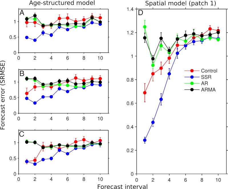
Similar results were obtained for the age-structured model. For the age 0 class, the short-term predictions of the SSR model were up to 50% better than the mean predictor, whereas the linear models and the control model were no better than a mean predictor. One-step-ahead predictions of the linear models for the age 1 and age 2 classes were consistently poor, whereas the control model prediction accuracy increased to that of the SSR method (Figs. 3 and 4).

Fig. 3.

Error of each forecasting method for the age-structured model (A–C) and patch 1 of the spatial model (D); similar results were obtained for patches 2–4 of the spatial model. For the age-structured model, ages 0, 1, and 2 are represented by A, B, and C, respectively. The red, blue, green, and black lines show the forecast error for the fitted control model, SSR model, AR model, and ARMA model, respectively.

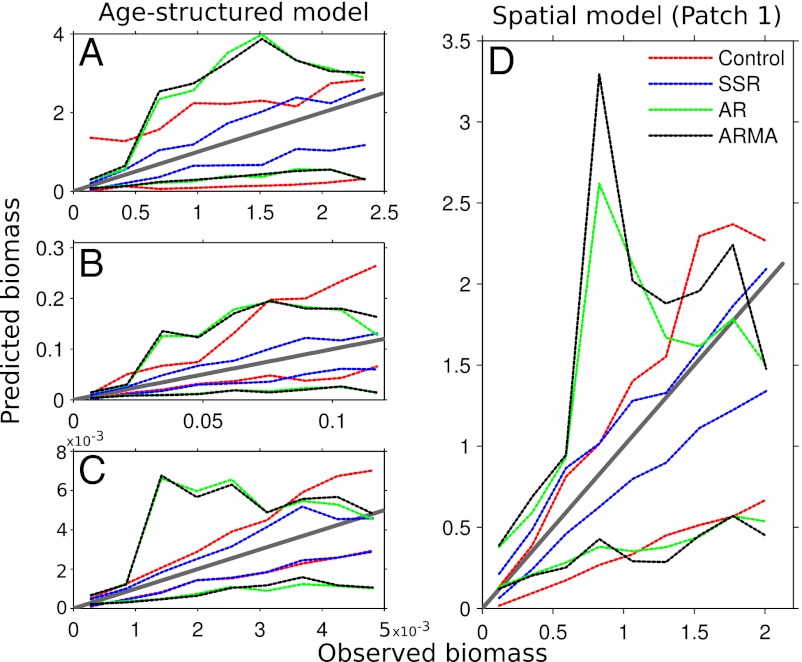
Fig. 4.

Predicted vs. observed for the age-structured (A–C) and spatial model (D). One-to-one line in gray (representing perfect predictions) and dotted lines showing 90% confidence intervals for each forecast method over all observations. The SSR model again provides the tightest confidence intervals about the one-to-one line.

The performance of the different forecasting methods varied widely for the spatial model. The SSR method again generated the most accurate predictions, with a forecast accuracy 70% better than the mean predictor. The control model provided short-term forecasts that were ∼50% better than the mean predictor, whereas the linear forecasting methods were no better than forecasting the mean (Figs. 3D and 4D).

Among the linear time series models, the simpler AR model provided a slightly better fit to the training set than the ARMA model (mean Akaike information criterion of −5.00 vs. −4.85 for the AR and ARMA models, respectively). Thus, the additional moving-average terms of the ARMA model were unable to capture the unexplained dynamics of the noisy, nonlinear models, which resulted in the slightly lower forecast error of the AR model (Figs. 1 and 3).

Experimental Data Methods

The holy grail of population biology is a model that both accurately predicts changes in abundance and can be used to anticipate critical thresholds. Through a battery of perturbation experiments and analyses of long time-series, this is exactly what was achieved in an extensive study of the flour beetle Tribolium castaneum (32). It was demonstrated that Tribolium population dynamics are well represented by a discrete, age-structured model of larvae, pupae, and adults (32–34), given as

where L_t is the abundance of feeding larvae at time t; P_t is the abundance of large larvae, nonfeeding larvae, pupae, and callow adults; and A_t is the number of sexually mature adults. The parameter b is the number of larval recruits per adult per unit of time in the absence of cannibalism, and the fractions μ₁ and μ_a are the larval and adult mortality rates, respectively. The exponential terms in the larvae equation describe the probability that an egg will be eaten in the presence of L_t−1 larvae and A_t−1 adults, and the exponential term in the adults’ equation describes the probability that a pupae will survive to become an adult when A_t−1 adults are present.

We used time series from the Tribolium experiments described in Dennis et al. (32) in which adult recruitment rates (for a total of seven treatments) were experimentally manipulated, producing limit cycles and chaos. For each experimental treatment, the population was censused every 2 wk for 80 wk, resulting in a 41-point time series. Each experimental treatment was replicated twice, providing three independent time series for each treatment with which to compare the forecast accuracy of the different methods. For each treatment, one time series was randomly chosen to fit the models (the training set), and the other two time series were used to evaluate forecast accuracy (the test set), providing a total of 21 evaluations.

To emulate ecologically realistic conditions, we added log-normal observation error with a CV of 0.2 to all of the training sets. The forecast accuracy was evaluated using the test-set time series without observation error. The larvae-pupae-adult (LPA) model was fit using the Bayesian MCMC routine described above with the parameter search initiated on the parameter values estimated in Dennis et al. (32) and on the correct initial conditions.

Experimental Results

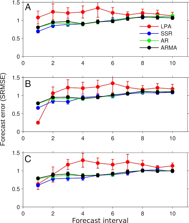
As with the simulation results, our analysis of the experimental data shows that the SSR time series method provided the most accurate short-term forecasts of all of the methods tested. When averaged over all treatments, short-term predictions (4 wk or less) made by the SSR method were significantly more accurate than the linear methods, and more accurate than the control model in all but one instance (Fig. 5). Short-term predictions (2 wk ahead) provided by the SSR method were routinely over 40% more accurate than a prediction of the mean of the time series (Fig. 5), whereas the linear methods were only ∼20% more accurate than a mean predictor.

Fig. 5.

Forecast error for the flour beetle experiments. Points represent the mean SRMSE over all experiments; bars are the SE. A, B, and C show results for the larvae, pupae, and adult test sets, respectively. In agreement with the simulations, the SSR method provided the most accurate forecasts overall.

Similar to the simulation results, although the MCMC routine for the control model had converged, it often converged on parameterizations that resulted in equilibrium dynamics when the true dynamics were either limit cycle or chaotic (Fig. S3); this resulted in poor prediction accuracy for the control model. The control model outperformed the time series methods only for the one-step predictions of the pupae stage, which is unsurprising given that the one-step-ahead transition from larvae to pupae is determined by a single mortality parameter.

For the longest prediction interval (20 wk), the forecast accuracy of all methods converged to that of the time series mean. Although this was expected for the chaotic treatments, due to sensitive dependence on initial conditions, it was notable that it also occurred for deterministic limit cycles and is likely due to the interaction of nonlinear dynamics and process noise.

For the larvae and adult time series, both the nonlinear (SSR) and linear methods (AR and ARMA) were significantly more accurate than the control model up to the 10-step-ahead prediction horizon (Fig. 5 A and C). The results for the pupae time series were similar, with the exception that the half-generation predictions of the control model were most accurate (Fig. 5B).

Discussion

Despite the absence of mechanistic information about the underlying ecological processes, the relatively simple SSR method consistently outperformed the control models over near-term prediction horizons. This result was robust across all simulations and all life stages of the experimental data. Moreover, the SSR model achieved this feat using only a single time series, whereas the control model used all times series simultaneously (it is an ecologically unrealistic scenario to assume we know the model and have time series for all of the relevant variables). Other analyses have shown that multivariate SSR methods (35) improve with additional information (14, 36), suggesting that the performance of the SSR model tested here represents a lower bound on forecast accuracy attainable with this general approach.

Overall, the control model forecast accuracy was similar to the SSR model for the linear components of the models. For example, for the linear (age 1 and age 2) components of the age-structured model, the short-term accuracy of the control model was similar to that of the SSR model, whereas the forecast accuracy of the control model for the nonlinear (age 0) component was significantly worse than the SSR model. Similar results were obtained for the experimental data because the control model provided the best forecasts for only the one-step-ahead predictions of the pupae stage, which is governed by a single linear mortality term. This finding suggests that the optimal forecasting model for age-structured populations may be one that combines a mechanistic model for the upper age classes with a time series model for the recruit dynamics.

For the cases considered here, we have shown that commonly used statistical procedures for fitting mechanistic models to chaotic time series will often converge on parameterizations that yield decidedly nonchaotic dynamics. In these cases, models with the wrong parameters will likely yield wrong inferences, and measures such as extinction risk, maximum sustainable yield, or population growth rate (Fig. S5) can be severely biased. This observation has particularly important implications for fishery management where mechanistic model-fitting is often a critical element of the assessment process.

An important question remains: How chaotic is too chaotic for traditional Bayesian methods? To address this question, we performed additional simulations for the logistic model under both chaotic and nonchaotic parameterizations (r = 2.5–3.95). The stability of the model strongly influenced parameter estimation error. Error grew rapidly as the model became unstable (Lyapunov exponent near zero; Fig. S1), and estimates of the Lyapunov exponent were severely biased toward stability (Fig. S2). This bias was present even when the true model was marginally stable, suggesting that our results are relevant even for nonchaotic systems in the presence of process error; we speculate that this may explain the apparent paucity of chaos in ecological time series. For a more detailed treatment of this question, see Judd (37).

Alternative model-fitting procedures have been proposed that estimate goodness of fit using summary statistics rather than directly estimating parameter likelihood (38, 39). However, those methods lack general recommendations for designing informative statistics for arbitrary dynamic systems, and therefore have not been widely adopted in ecology. Another promising method involves fitting semiparametric functions to first-differenced data (40); however, that method is considerably more challenging to implement than the model-free methods described here, and it has not been widely tested or adopted.

As ecologists, our ultimate goal is to uncover the processes that govern natural systems. The ideal route to such discovery is through hypothesis testing via controlled experiments. Unfortunately, population-level hypotheses are impossible to test through such experiments, and moreover, ecosystem dynamics are often sufficiently complex that perturbation of any single variable is unlikely to yield great insight. Forecasting provides a way forward, because population-level hypotheses can be evaluated based on our ability to make accurate predictions. Importantly, however, even correct models with the correct parameters will fail to provide accurate long-term forecasts due to sensitive dependence on initial conditions and nonstationarity. Therefore, it would be fruitful for future work to determine how to use short-term forecasts, which can be validated empirically, to ensure sustainability in a changing environment.

References

- 1. Volterra V (1926) Fluctuations in the abundance of a species considered mathematically. Nature 118(2972):558–560.
- 2.May RM. Simple mathematical models with very complicated dynamics. Nature. 1976;261(5560):459–467. doi: 10.1038/261459a0. [DOI] [PubMed] [Google Scholar]
- 3.Reed DH, Hobbs GR. The relationship between population size and temporal variability in population size. Anim Conserv. 2004;7(1):1–8. [Google Scholar]
- 4.Pimentel D, Lach L, Zuniga R, Morrison D. Environmental and economic costs of nonindigenous species in the united states. Bioscience. 2000;50(1):53–65. [Google Scholar]
- 5.Doak DF, et al. Understanding and predicting ecological dynamics: Are major surprises inevitable? Ecology. 2008;89(4):952–961. doi: 10.1890/07-0965.1. [DOI] [PubMed] [Google Scholar]
- 6.Clark JS, et al. Ecological forecasts: An emerging imperative. Science. 2001;293(5530):657–660. doi: 10.1126/science.293.5530.657. [DOI] [PubMed] [Google Scholar]
- 7.Buckland S, Newman K, Thomas L, Koesters N. State-space models for the dynamics of wild animal populations. Ecol Modelling. 2004;171(1):157–175. [Google Scholar]
- 8.Clark JS, Bjornstad ON. Population time series: Process variability, observation errors, missing values, lags, and hidden states. Ecology. 2004;85(11):3140–3150. [Google Scholar]
- 9.Wood SN, Thomas MB. Supersensitivity to structure in biological models. Proc R Soc Lond B Biol Sci. 1999;266(1419):565–570. [Google Scholar]
- 10.Holmes EE, Sabo JL, Viscido SV, Fagan WF. A statistical approach to quasi-extinction forecasting. Ecol Lett. 2007;10(12):1182–1198. doi: 10.1111/j.1461-0248.2007.01105.x. [DOI] [PubMed] [Google Scholar]
- 11.Lindegren M, et al. Ecological forecasting under climate change: The case of Baltic cod. Proc Biol Sci. 2010;277(1691):2121–2130. doi: 10.1098/rspb.2010.0353. [DOI] [PMC free article] [PubMed] [Google Scholar]
- 12.Dakos V, et al. Slowing down as an early warning signal for abrupt climate change. Proc Natl Acad Sci USA. 2008;105(38):14308–14312. doi: 10.1073/pnas.0802430105. [DOI] [PMC free article] [PubMed] [Google Scholar]
- 13.Sugihara G. 1994. Nonlinear forecasting for the classification of natural time series. Phil Trans R Soc Lond A 348(1688):477–495.
- 14.Dixon PA, Milicich MJ, Sugihara G. Episodic fluctuations in larval supply. Science. 1999;283(5407):1528–1530. doi: 10.1126/science.283.5407.1528. [DOI] [PubMed] [Google Scholar]
- 15.Kantz H, Schreiber T. Nonlinear Time Series Analysis. Cambridge, UK: Cambridge Univ Press; 2004. [Google Scholar]
- 16.Satoh K, Aihara T. Numerical study on a coupled-logistic map as a simple model for a predator-prey system. J Phys Soc Jpn. 1990;59:1184–1198. [Google Scholar]
- 17.Levin SA, Goodyear CP. Analysis of an age-structured fishery model. J Math Biol. 1980;9:245–274. [Google Scholar]
- 18.Hastings A, Wysham DB. Regime shifts in ecological systems can occur with no warning. Ecol Lett. 2010;13(4):464–472. doi: 10.1111/j.1461-0248.2010.01439.x. [DOI] [PubMed] [Google Scholar]
- 19.Francis RC, Hurst R, Renwick J. Quantifying annual variation in catchability for commercial and research fishing. Fish Bull. 2003;101(2):293–304. [Google Scholar]
- 20.Geyer CJ. 1991. Computing Science and Statistics: Proceedings of the 23rd Symposium on the Interface, ed Keramigas EM (Interface Foundation of North America, Fairfax Station, VA), pp 156–163.
- 21.The MathWorks, Inc. 2011. MATLAB version 7.12.0 (R2011a) (The MathWorks Inc., Natick, MA)
- 22.R Development Core Team . R: A Language and Environment for Statistical Computing. Vienna: R Foundation for Statistical Computing; 2011. [Google Scholar]
- 23.Plummer M. 2003. JAGS: A program for analysis of Bayesian graphical models using Gibbs sampling. Proceedings of the Third International Workshop on Distributed Statistical Computing. Available at www.r-project.org/conferences/DSC-2003/Proceedings/index.html.
- 24.Gelman A, Rubin DB. Inference from iterative simulation using multiple sequences. Stat Sci. 1992;7(4):457–472. [Google Scholar]
- 25.King R. Bayesian Analysis for Population Ecology. Boca Raton, FL: CRC; 2009. [Google Scholar]
- 26.Polansky L, de Valpine P, Lloyd-Smith JO, Getz WM. Likelihood ridges and multimodality in population growth rate models. Ecology. 2009;90(8):2313–2320. doi: 10.1890/08-1461.1. [DOI] [PubMed] [Google Scholar]
- 27.Takens F. 1981. Detecting strange attractors in turbulence. Dynamical Systems and Turbulence: Warwick 1980, eds Rand D, Young LS (Springer, New York), pp 366–381.
- 28.Hsieh CH, Glaser SM, Lucas AJ, Sugihara G. Distinguishing random environmental fluctuations from ecological catastrophes for the North Pacific Ocean. Nature. 2005;435(7040):336–340. doi: 10.1038/nature03553. [DOI] [PubMed] [Google Scholar]
- 29. Anderson C, Sugihara G (2006) Simplex portal. Available at http://simplex.ucsd.edu/
- 30.Stark J, Broomhead D, Davies M, Huke J. Delay embeddings for forced systems. II. stochastic forcing. J Nonlinear Sci. 2003;13(6):519–577. [Google Scholar]
- 31.Box G, Jenkins G, Reinsel G. Time Series Analysis: Forecasting and Control. 3rd Ed. Englewood Cliffs, NJ: Prentice Hall; 1994. [Google Scholar]
- 32.Dennis B, Desharnais RA, Cushing JM, Henson SM, Costantino RF. Estimating chaos and complex dynamics in an insect population. Ecol Monogr. 2001;71(2):277–303. [Google Scholar]
- 33.Dennis B, Desharnais RA, Cushing JM, Costantino RF. Nonlinear demographic dynamics: Mathematical models, statistical methods, and biological experiments. Ecol Monogr. 1995;65(3):261–282. [Google Scholar]
- 34.Desharnais RA, Costantino RF, Cushing JM, Henson SM, Dennis B. Chaos and population control of insect outbreaks. Ecol Lett. 2001;4(3):229–235. [Google Scholar]
- 35.Deyle ER, Sugihara G. Generalized theorems for nonlinear state space reconstruction. PLoS ONE. 2011;6(3):e18295. doi: 10.1371/journal.pone.0018295. [DOI] [PMC free article] [PubMed] [Google Scholar]
- 36.Cao L, Mees A, Judd K. Dynamics from multivariate time series. Physica D. 1998;121(1):75–88. [Google Scholar]
- 37.Judd K. Failure of maximum likelihood methods for chaotic dynamical systems. Phys Rev E Stat Nonlin Soft Matter Phys. 2007;75(3 Pt 2):036210. doi: 10.1103/PhysRevE.75.036210. [DOI] [PubMed] [Google Scholar]
- 38.Wood SN. Statistical inference for noisy nonlinear ecological dynamic systems. Nature. 2010;466(7310):1102–1104. doi: 10.1038/nature09319. [DOI] [PubMed] [Google Scholar]
- 39.Hartig F, Calabrese JM, Reineking B, Wiegand T, Huth A. Statistical inference for stochastic simulation models—theory and application. Ecol Lett. 2011;14(8):816–827. doi: 10.1111/j.1461-0248.2011.01640.x. [DOI] [PubMed] [Google Scholar]
- 40.Ellner SP, Seifu Y, Smith RH. 2002. Fitting population dynamic models to time-series data by gradient matching. Ecology 83(8):2256–2270.
Associated Data
This section collects any data citations, data availability statements, or supplementary materials included in this article.