Estimating Spatiotemporal Variability of Ambient Air Pollutant Concentrations with A Hierarchical Model

Abstract

Studies have linked exposure to air pollutants to short-term and sub-chronic health outcomes. However, individual-level air pollution exposure is difficult to measure at a high spatial and temporal resolution and for larger populations due to limitations in sampling techniques. We presented a hierarchical model to capture spatiotemporal variability of nitrogen dioxide (NO₂) and nitrogen oxides (NO_x) concentrations in Southern California by combining high temporal resolution data from routine monitoring stations with high spatial resolution data from investigator-initiated episodic measurements. In this model, the spatiotemporal field of concentrations was first decomposed into a mean and residual and the mean representing the seasonal trend was further decomposed into a constant and varying temporal basis functions. The mean of the spatially varying coefficients of temporal basis functions were modeled by local covariates using non-linear generalized additive model and least square fitting using measurements from both routine monitoring and additional episodic sampling locations, while the spatially-correlated residuals of the coefficients were co-kriged. We found traffic, land-use and wind accounted for a large portion of the variance (beyond 35%) for the long-term average trend of concentrations. Spatial residuals accounted for a large portion of the variance of the temporal components (about 30% for NO₂ and 20% for NO_x). Leave-one-out cross validation produced an R² of 0.84 for NO₂ and 0.81 for NO_x when comparing the modeled weekly concentration with the observed trends at all routine monitoring stations.

1. Introduction

Exposures to air pollution have been linked to short-term and sub-chronic adverse health outcomes, including daily respiratory and cardiovascular morbidity (Mahiyuddin et al., 2013; Zanobetti et al., 2003), and adverse pregnancy outcomes (Ritz and Wilhelm, 2008). Many time-series health effect studies relied solely on area-wide exposure measures that failed to account for spatial exposure variability among individual subjects, and thus may have underestimated the magnitude of estimated effects (Lindstrom et al., 2011). For urban areas with spatially heterogeneous emission sources (e.g. Los Angeles, California), the within-area variation of air pollutant concentrations was possibly larger than the between-area variations (Jerrett et al., 2005). In these areas, it is essential to account for individual-level exposure variation in air pollution epidemiological studies.

Spatial proximity, spatial interpolation, and land use regression (LUR) models have been extensively used to assign exposure estimates to individual subjects that are more spatially refined but generally ignore temporal patterns of variation. Some studies assign measurements taken at the nearest monitoring station to a target location. This approach usually allows one to generate exposure estimates at a moderate or high temporal resolution while the spatial resolution is relatively low due to the limited coverage of the routine monitoring stations. Spatial interpolation (e.g. kriging) derives unbiased exposure estimation based on the existing measurements (Whitworth et al., 2011) with no additional spatial information used; spatial resolution is thus still limited by the number of routine sampling sites. The LUR models incorporate local covariates, including land-use/cover, population, and traffic information, to predict intra-urban variation of air pollution based on measurements at a high spatial resolution (Jerrett et al., 2005). Most previous LUR models focused on characterizing long-term spatial (Hart et al., 2009) or seasonal exposures (Li et al., 2012) and had no or low temporal resolution (Hoek et al., 2008). Some studies superimposed temporal profiles from routine monitoring stations onto the long-term LUR-estimated concentrations (Ghosh et al., 2012). These approaches may be inadequate because they typically rely on measurements at fewer locations than used to develop the models themselves or/and assume that temporal changes are constant across the study area (Wu et al., 2011). Jerrett et al. (2012) applied LUR models repetitively on monthly measurements of particulate matter <2.5 μm; Bayesian maximum entropy (BME) was further used to estimate spatiotemporal variability of the residuals of LUR-estimated monthly means. BME is a local spatiotemporal modeling approach that incorporates measurement data, prior knowledge of neighbor information, and local spatiotemporal covariates. This study, however, did not systematically integrate temporal variability in the models.

Only a few studies have systematically modeled spatiotemporal variability of air pollutants at a high spatial and temporal resolution. BME was developed to estimate the spatiotemporal concentrations of particulate matter <10 μm and ozone (Yu et al., 2009). Two-stage models were developed for particulate matter with a second-order stationary and isotropic assumption of spatiotemporal covariance and linear regression to correlate the covariates to spatiotemporal trend of concentrations (Cameletti and Ignaccolo, 2010). Szpiro et al. (2010) constructed a hierarchical model for nitrogen oxides (NO_x) with a flexible correlation structure and spatial stationary assumption. Lindstrom et al. (2011) adapted the hierarchical model used in Szpiro et al. (2010) by adding a spatiotemporal covariate (i.e. estimated concentration from a line-source dispersion model).

Most spatiotemporal models were trained using the routine monitoring data. In this paper, we presented a hierarchical model that fully utilizes all available measurements (both long-term data at routine monitoring stations and additional short-term data from the investigator-initiated field campaigns) and spatial covariates to reliably estimate spatiotemporal variability of pollutant concentrations. The U.S. Environmental Protection Agency (EPA) monitoring network provides long-term measurements for the criteria air pollutants at a high temporal resolution throughout the country, although the sampling stations are usually sparsely located. Investigator-initiated field campaigns, on the other hand, usually have a relatively dense spatial coverage, but are often short-term and passive sampling only for one or two types of pollutants. In this study, we developed hierarchical two-stage models based on a couple of previous studies (Finkenstadt et al., 2007; Szpiro et al., 2010) that combined dominant temporal trends at regional scale with spatial variability at local scale to improve estimation of spatiotemporal variability of pollutant concentrations. The models were developed for nitrogen dioxide (NO₂) and NO_x, two criteria air pollutants widely used in air pollution health studies (Jerrett et al., 2012).

2. Materials

2.1. Study domain

This study covers the metropolitan Los Angeles area (160 × 161 km²; over 12 million in population in 2010) including both Los Angeles and Orange counties in Southern California. This region has serious air pollution problems due to high emissions (e.g. traffic, industrial and port-related activities), unfavorable meteorology, and high population density. There are six major commuter and truck transport freeways within this densely populated region.

2.2. NO₂ and NO_x measurements

2.2.1. Long-term routine measurements from government-operated monitoring stations

We obtained routine measurements of hourly NO₂ and NO_x concentrations (unit: ppb) from 2006 to 2009 from the South Coast Air Quality Management District (SCAQMD) monitoring network at 32 stations in Southern California. The measurements were conducted by federally designated automated chemiluminescence methods with actively sampling instruments. Weekly average concentrations were calculated based on hourly data using a 75% completeness criterion; a total of 209 weekly concentrations were calculated from January 2006 to December 2009. Figure 1 shows the SCAQMD monitoring stations in the study domain. Among the 32 SCAMQD stations, one station was excluded because of the extreme values observed at this station based on the criteria of outer fences (Iglewicz and Hoaglin, 1993). Weekly concentrations from the 25 routine stations with complete (<3% missing values) time series data were used in the first stage of the hierarchical model to estimate the trend of constant and varying temporal basis functions. The measurements from the rest 6 stations (excluding the one having outliers) were used as episodic measurements due to more missing values (>3%).

Figure 1.

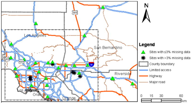
Study domain with 31 SCAQMD sites (25 sites with ≤3% missing data used for generating temporal basis functions of the domain and 6 sites with >3% missing data; all SCAQMD sites used for spatial modeling with UCI and UCLA measurements)

2.2.2. Episodic measurements

Besides the measurements with >3% missing values from the 6 SCAQMD sites, episodic measurements include 161 valid NO₂ and NO_x samples from University of California, Los Angeles (UCLA) (collected in two continuous weeks, i.e. September 16-October 1, 2006 and February 10–25, 2007) and 32 valid samples of measurements for NO₂ and NO_x from University of California, Irvine (UCI) (collected at outdoor home locations of subjects in south Los Angeles and Orange counties for four weeks, i.e. July 10–18, July 24-August 1, November 13–21 and December 4–12 in 2009). For details of episodic measurements from UCI and UCLA, and their adjustment for use in combination with SCAQMD routine data, please refer to Supplemental Materials Section 2.1 and Table S1.

2.3. Spatial covariates

2.3.1. Covariates related to emission

Emission sources contribute significantly to the variability of pollutant concentrations. Traffic was one of the major sources of air pollution in the Los Angeles area. Land-use data were used as surrogates of traffic and other emissions.

1. Roadway covariates include total roadway length (meter) inversely weighted by the distance to the sampling location within an optimal buffer size as well as the shortest distances (meter) from the sampling location to each of four roadway types, and all the four type of roadways (highway as A1, primary roads as A2, secondary or connecting roads as A3 and local roads as A4, see Supplemental MaterialsSection 2.2 for details). To estimate the optimal buffering distance, Pearson’s correlations between the distance-weighted roadway length and the concentrations were calculated within the buffers of increasing radii (from 50 m to 5 km with interval of 50 m or 100 m); an optimal buffering distance had the highest correlation. We used 5 km as a threshold since a wider buffering distance might include influence from background and regional sources. This method was also used for the other spatial covariates that required buffer statistics. The ESRI StreetMap^™ North America 9.3 (http://www.esri.com) including 2003 TeleAtlas^® street polylines was used as the roadway data.

2. Traffic flow. We obtained annual average daily traffic (AADT) counts in 2005for all the freeways, highways, and major surface streets from the California Department of Transportation (Caltrans). AADT was weighted by the roadwaylength with in an optimal buffer.

3. Land-use covariates. Land-use data were obtained from the Southern California Association of Government (SCAG). The original 108 land-use types were classified into five major categories: transportation, industry, agriculture including open space and vacant, commercial area, and residential area. We calculated the percentage of area for each land-use category within an optimal buffer size.

2.3.2. Meteorologicalc ovariates

Long-term meteorological covariates were derived by averaging multiple-year (2006–2009) measurements of temperature (°C), wind speeds (meters/second abbreviated as m/s), wind direction, relative humidity (%), and precipitation (inch) from the Air Quality and Meteorological Information System managed by the California Air Resources Board (http://www.arb.ca.gov/aqmis2/aqmis2.php). Wind data were decomposed into two vectors by respectively multiplying wind speed with sine and cosine of wind direction, with the sine value positive from the east and the cosine value positive from north) (Carslaw et al., 2007). There were 67 sites for temperature, 77 sites for wind speed and wind direction, 37 sites for relatively humidity, and 55 sites for precipitation. Measurements at the nearest meteorological site were assigned to the corresponding sampling location.

2.3.3. Other location-related covariates

We obtained elevation data at 10m×10m resolution from US National Elevation Dataset (NED) (http://nationalmap.gov/) and assigned the elevation (meter) to each sampling location. We also calculated the shortest distance (meter) to shoreline for each sampling location.

3. Modeling approach

3.1. Stage one: decomposition of spatiotemporal field

A normally-distributed log-transformed spatiotemporal field y_ut (u=1,…,n site; t=1,…,m time slice) was decomposed into the sum of a systematic mean component (μ_ut) and residual (ε̂_ut) (Finkenstadt et al., 2007):

$$y_{ut}={\mu }_{ut}+{\widehat{\epsilon }}_{ut}$$ [1]

The mean spatiotemporal field typically represents the dominant seasonal or long-term trend of concentrations for the study domain (Szpiro et al., 2010). At the first stage, the mean component was divided into one constant and two varying temporal basis functions using the empirical orthogonal functions (EOFs) (a.k.a. independent temporal basis functions) and the long-term weekly concentrations from the 25 SCAQMD routine monitoring stations. EOFs were often used to present leading modes of variability in space-time processes in meteorology; their smoothed curves are often used to reduce noise (Finkenstadt et al., 2007). In [1], the mean μ_ut is essentially a projection of time series at the location, u onto the space spanned by the constant temporal basis function (represented by β_0u) and varying ones f_i(t) (i=1,…,m) and corresponding spatially varying coefficient β_iu at u for f_i(t):

$${\mu }_{ut}={\beta }_{0u}+{\beta }_{1u}{f}_1(t)+{\beta }_{2u}{f}_2(t)+\cdots +{\beta }_{mu}{f}_m(t)(u=1,\dots ,n;t=1,\dots ,m)$$ [2]

where β_0u is an intercept (f₀(t)≡1) representing spatial variability of the constant temporal basis function. Similarly, the coefficient, β_1u (β_2u) representing spatial variability of the first (second) temporal basis function. In [1], ε̂_ut ~ N(0, σ), independent of μ_ut, is assumed to be spatially correlated after removal of temporal auto-correlation and it can be modeled using kriging. Autocorrelation function (ACF) and partial autocorrelation function (PACF) were used to test the temporal autocorrelation of the residuals. We found that the ACF and PACF values were generally below 0.3, indicating very weak temporal autocorrelation of the residuals.

In [2], singular value decomposition (SVD) was used to generate the independent temporal basis functions. Iterative SVD (Finkenstadt et al., 2007) was also used to fill 1–5 temporal missing values (<3%) for 13 routine SCAQMD stations. The derivative-based thin plate spline penalty was applied to select a good degree of freedom to fit the temporal basis functions. With a good degree of freedom, the smoothed curve will properly represent the true temporal trend and meanwhile minimize over-fitting (Szpiro et al., 2010). We used Wood (2002)’s integrated approach of model selection and automatic smoothing parameter selection to select the degree of freedom with generalized cross-validation (GCV) criterion to determine the smoothing parameters for the temporal basis functions. More details about the temporal basis functions can be found in Supplemental Materials Section 2.3.

3.2. Stage Two: estimation of spatially varying coefficients for independent temporal basis functions

At this stage, spatially varying coefficients at the routine stations and episodic sampling sites were estimated using ordinary least square technique. We then applied a non-linear generalized additive model (GAM) plus cokriging to model these coefficients using local spatial covariates.

The product of the first three coefficients in [2], β_iu (i=0, 1, 2) and their temporal basis functions can usually capture the majority of spatiotemporal variability of concentrations (Lindstrom et al., 2011; Szpiro et al., 2010). In practice, we only need to solve the following linear equations to estimate the three coefficients at u, assuming observed values of L time slices for u:

$$y_{ut}={\mu }_{ut}+{\epsilon }_{ut}={\beta }_{0u}+{\beta }_{1u}{f}_1(t)+{\beta }_{2u}{f}_2(t)+{\epsilon }_{ut}(t=1,\dots ,L)$$ [3]

Since ε_ut is independent of μ_ut, (ε_u ~ N(0,1)), we used the least square fit to solve β_iu (i=0, 1, 2). A unique solution for β_iu (i=0, 1, 2) is possible in equation [3] if we have a minimum of three time slices of measurements at each sampling location according to the Rouché–Capelli theorem (David, 2006).

The UCI and SCAQMD data had at least four weekly measurements and were directly used to solve the β_i coefficients in [3]. But the UCLA data had only two bi-weekly measurements, fewer than a minimum of three required to solve β_iu (i=0, 1, 2). Thus, the initial ratios between the two continuous weekly averages of concentration and the ratios were estimated using the linear spatiotemporal model and then used to interpolate four weekly concentration averages from two bi-weekly measures of concentration averages. In this spatiotemporal model, we derived temporal basis functions and spatial coefficients using the 25 routine measurements of time series (no episodic data were used) and estimated the spatial coefficients based on two or three significant spatial covariates (roadway length, AADT or traffic land-use, and wind speed). We then estimated two continuous weekly concentrations at the UCLA sampling locations and the initial ratios respectively for 2006 and 2007. The procedure was based on maximum likelihood without the incorporation of spatial autocorrelation of residuals (Supplemental Materials Section 2.4).

Sensitivity analysis was conducted to examine the influence of the interpolation methods on model performance. We compared the interpolation method above (i.e. linear spatiotemporal model) with two other methods. One method assigned the two-week average concentration to each of the two individual weeks, assuming no variation in the concentrations over the two continuous weeks (i.e. initial ratio =1). The other one used the ratio of two weekly measurements at the nearest SCAQMD station to split the data, assuming that the ratio of concentrations at the nearest station properly reflected the variation of concentrations over the two continuous weeks.

3.2.1 Removal of outliers in episodic measurements

Outliers from episodic samples may affect the estimation of β_iu (i=0, 1, 2). We estimated β_i of the 25 routine stations, which were then used as the reference values to exclude the outliers in episodic measurements. The outer fences (Iglewicz and Hoaglin, 1993) of β_i were used to filter the outliers. A data point was treated as an outlier if the value of β_i was outside the outer fences (Q1-3*IQR, Q3+3*IQR; Q1 and Q3 are respectively the first and third quartiles, and IQR is inter-quartile range). In total, we excluded 8 outliers (4 from UCLA and 4 from UCI) for NO₂ and 6 outliers from UCI for NO_x.

The removal of too few outliers may cause poor model performance, while the removal of too many outliers may over-fit the model. Sensitivity analysis was conducted for three different definitions of outliers for β_i: 1) No outliers removed from the UCI and UCLA samples (reference); 2) Inner fences used to remove outliers (Q1-1.5*IQR, Q3+1.5*IQR); 3) Outer fences as less conservative criteria to remove outliers, introduced above and used in this study (Supplemental Materials Table S6). Compared to the models with no outlier removal, the removal of outliers improved the model performance by 5% to approximately 20% (Supplemental Materials Table S6).

3.2.2. GAM: modeling local mean of spatially varying coefficients

The GAM equation for prediction of spatially varying coefficients for temporal basis functions is:

$${\widehat{\beta }}_{iu}={\widehat{\overline{\beta }}}_{iu}(X)+{\widehat{\epsilon }}_{\mathit{ius}}(Z)+{\widehat{\epsilon }}_{\mathit{iun}}$$ [4]

where β̂_iu (i=0, 1, 2) is estimate of spatially varying coefficient for the i^th basis function at location u, ${\widehat{\overline{\beta }}}_{\text{iu}}$ is the estimate of local mean at u for β̂_iu, dependent on the set of p spatial covariates, $X=\{x_u^j\}(j=1\dots p)$, ε̂_iusis the estimate of spatial residual for β̂_iu, determined by spatial residuals of samples that belong to the neighborhood of u, Z ∈ Nb(u), ε̂_iun is a random residual at u, with normal distribution, ε̂_iun ~ N(0,1).

We used the GAM package in R statistical software (Version 2.11.1) to develop and validate the model. The following is to correlate local spatial covariates to the mean of β̂_iun:

$$g\left(E({\widehat{\beta }}_{iu})\right)={\mu }_{i0}+{\sum }_{j=1}^q{s}_j(x_u^j)+s_w(w\_s_u,w\_c_u)+{\sum }_{k=q+1}^p{\gamma }_k{x}_u^k$$ [5]

where μ_io is the model intercept, w_s_u ([wind speed] ·sine([wind direction]) and w_c_u ([wind speed] · cosine([wind direction]) respectively represent two wind vectors, at u, $x_u^j$ or ${\text{x}}_{\text{u}}^{\text{k}}\in \text{X}$ are other local covariates, s_j(…) is the smooth function to model the non-linear relationship between $x_u^j$ and $g\left({\widehat{\overline{\beta }}}_{iu}\right)$, s_w(w_s_u, w_c_u) is a bivariate smooth function to model the interaction between wind speed and wind direction, γ_k are the linear parameters used to construct the linear relationship between ${\text{x}}_{\text{u}}^{\text{k}}$ and g(E(β̂_iu)), and p is the number of covariates. For normally distributed β̂_iu(i=0, 1, 2), the link function is g(E(β̂_iu)). If β̂_iu does not follow the normal distribution, a power transformer can be used to make them normal (Handelsman, 2002). For the degree of freedom in non-linear fitting of β̂_i, we applied the same approach that was used to fit the temporal basis functions.

For selection of covariates, we first used Pearson’s correlation of 0.1 as a threshold to filter out the irrelevant ones and then selected optimal covariates by examination of multi-colinearity and combinational tests. See Supplemental Materials Section 2.5 for details.

3.2.3 Kriging of residuals to minimize error variance

Spatial residuals ε̂_ius in [4] were modeled by cokriging them with regional residuals at nearby samples with the assumption of a stable spatial domain after removal of local means (Christakos, 1990). Assuming ε = [ε_us|rs(u_i)]~N(0,V(θ))(i = 0, 1, 2, …f), u₀ is the location to be estimated, θ is the vector of variogram parameters (characterized by range ф, partial sill, σ² and optional model efficient, τ; nugget supposed to be 0 given the assumption of highly spatial correlation), Z = {u₁,u_2, … …, u_f} is the set of spatial samples belonging to the neighborhood of u₀; ε̂_us(u_i) is the estimate of spatial residual at the neighboring location, u_i, and is derived by subtracting the GAM local mean from β_kui at a sampling location; ε̂_rs(u_i) is the estimate of the regional residual or total variation of β_kui at the regional scale and derived by subtracting the population’s mean from β_kui at each sampling location. Cokriging used maximum likelihood based on estimates of variogram, θ and we can get the estimate of the residual for u₀:

$${\widehat{\epsilon }}_{us}(u_0)={\sum }_{i=1}^{n_u}{\lambda }_{u_i}^u{\widehat{\epsilon }}_{us}(u_i)+{\sum }_{i=1}^{n_u}{\lambda }_{u_i}^r{\epsilon }_{rs}(u_i)$$ [8]

where ${\lambda }_{u_i}^u$ and ${\lambda }_{u_i}^r$ are the optimal cokriging weights estimated according to the minimum unbiased optimal principle of Kriging.

3.3. Cross validation

For model evaluation, we used leave-one-out cross validation (LOOCV), which used an observation as the validation data and the remaining observations as the training data. This is repeated such that each observation in the sample is used once as the data point for which the validation is performed. In LOOCV, we validated how the estimated trend of concentrations captured spatiotemporal variability of the observed time series for the 25 routine SCAQMD stations, by measuring the 95% confidence intervals of Pearson’s correlations of time series for the 25 stations and R² for all the temporal trends of all the stations. We compared our approach with the spatiotemporal model based on linear regression (Finkenstadt et al., 2007). Further, we calculated R² of the estimated versus observed averages of the concentrations over 4 years (2006–2009) and the corresponding square root of the mean of the squared errors (RMSE).

4. RESULTS

4.1. Temporal basis functions and their spatially varying coefficients

Figure 2 depicts the first two varying temporal basis functions as trend curves smoothed by GAM for the study domain. The first component (product of temporal basis function and its spatially varying coefficient; the temporal trend alone unable to reflecting its seasonal trend) of the temporal basis trends showed clear seasonal changes, i.e. high in the winter and low in the summer. For NO₂, the first component of temporal basis trend accounted for 59% of variance. For NO_x, the first component accounted for 56% (except outliers, its spatially varying coefficient, β₁ generally smaller than 0, Supplemental Materials Table S3). The trend of the second temporal basis function explaining a much lower percentage of variance (about 9% for NO₂ and 9% for NO_x), was inconsistent with the seasonal trend, and seemed more complicated. Supplemental Materials Table S3 lists the descriptive statistics of β_i generated by least square fitting based on all routine and episodic measurement data. Supplemental Materials Figure S1 presents the box plots.

Figure 2.

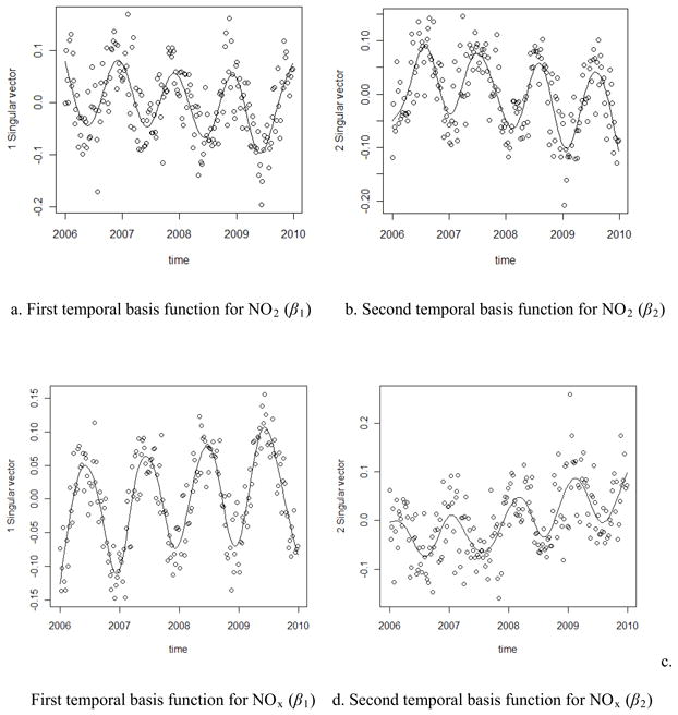
Plots of the first and second independent temporal basis functions for NO₂ and NO_x

4.2. Step one of spatial modeling: correlate local covariates to spatially varying coefficients

Table 1 lists the variances explained in total and by local covariate and spatial autocorrelation of the residuals. Figure 3 shows the non-linear relationship of change trend between smoothed β₀ and traffic factors, land-use and long-term average wind covariate with the 95% confidence intervals (the gray area). Supplemental Materials Figure S2–S7 show the changing trends between β_i and the covariates used as regressors.

Table 1.

Statistics of fit parameters by the routine time series and sporadic samples

Statistics	NO2			NOx
	β0	β1	β2	β0	β1	β2
Min	0.59	0.02	−12.80	0.69	−16.09	−9.37
Max	3.46	20.96	9.93	4.32	−0.43	11.04
Mean	2.90	0.33	0.33	3.51	−9.24	0.86
Variance	0.13	8.08	10.16	0.20	6.90	14.11
Median	3.00	5.29	−0.16	3.62	−9.27	1.07

Figure 3.

Influence of traffic, land-use and wind covariates for spatially varying coefficient, β ₀ of the NO₂ and NO_x constant temporal basis functions (the variance explained in the parenthesis)

For β₀, significant local covariates included traffic-related factors (AADT, distance-weighted roadway length, traffic land-use or distance to roadways), meteorological covariate (long-term ambient wind covariate), shortest distances to the shorelines, land-use area proportions (residential, commercial or agricultural/open field) or elevation. Traffic factors together accounted for an important part of variance (32.9% for NO₂ and 19% for NO_x). Except for traffic land-use, other land-use factors together accounted for about 17% of variance for NO₂ or 10% for NO_x. Major traffic-related factors, residence land-use and shortest distance to shorelines present positive correlation with β₀. Wind speed and wind direction were an important predictor, accounting for about 20.2–34.5% of variance. Lower wind speed was associated with higher β₀, while wind from the northwest was associated with lower β₀ (Figure 3e and 3f). Elevation and shortest distance to the shorelines together explained 13.0% of the variance for NO₂ and 19.9% for NO_x.

For β₁, the NO₂ variance was more influenced by long-term average wind (25.2%), land-use covariates (22.2%) and traffic-related factors (8.0%), while the variance of NO_x was more explained by long-term average wind (22.1%), weighted road length (15.4%) and land-use (24.6%). Wind from the north had stronger influence on NO₂, while wind from the west had more influence on NO_x.

For β₂, the variance of NO₂ was more influenced by long-term average wind (21.1%), commercial land-use (14.3%) and distance-weighted road length (6.8%), while the variance of NO_x was more explained by long-term average wind (33.5%), elevation (14.3%) and traffic-related factors (16.8%; including traffic land-use). The south wind had major contribution for β₂ of NO₂.

4.3. Step two of spatial modeling: variogram of spatial residuals

Although only explaining a small-modest part of variance for β₀ (4.2–8%), spatial autocorrelation of the residuals for β₁ and β₂ accounted for a considerable proportion of the variance explained 19.4–31.8% (Table 1). Supplemental Materials Table S4 shows the variogram models and relevant coefficients for spatial residuals of β_i. We found that β₀ for the constant basis function had a longer range and smaller partial sills, indicating a more gradual spatial variability. β₁ and β₂ of the varying temporal basis functions had a shorter range and higher partial sills, indicating higher spatial variability, probably more affected by wind.

4.4. Comparison of modeled vs. observed temporal trend

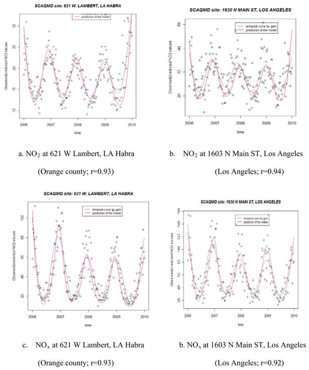
Figure 4 shows the typical curves of two SCAQMD stations (one in Orange County and the other in Los Angeles County) simulated with our method based on the time series data at the other 24 SCAQMD stations and episodic measurement data vs. the practical smoothed curves derived from the observed time series. The simulated curves and the observed values showed a strong association. For the temporal trends of the 25 routine SCAQMD stations, the median of the correlation between the LOOCV predicted values and observed time series was 0.90 (mean: 0.87) with the 95% confidence interval (CI) of [0.83, 0.91] for NO₂ and 0.96 (0.92) with 95% CI of [0.88, 0.96] for NO_x.

Figure 4.

Good match between observed values vs. simulated values for NO₂ and NO_x (r: correlation)

For all 5225 (25×209) weekly samples, our model had a CV R² of 0.67 for NO₂ and 0.66 for NO_x between the predicted time series and observed values, but the model had a better CV R² (0.84 for NO₂; 0.81 for NO_x) between our predicted time series and the GAM-smoothed trend curves of weekly measurement data. Our model outperformed the linear spatiotemporal model in predicting the smoothed trend curve (0.84 vs. 0.56 for NO₂; 0.81 vs. 0.65 for NO_xin Table 2).

Table 2.

Explained variance and influence of local covariates and spatial autocorrelation for estimation of parameters (p-value<0.1)

Statistics	NO2						NOx
	β0		β1		β2		β0		β1		β2
	Coef	V.E.	Coef	V.E.	Coef	V.E.	Coef	V.E.	Coef	V.E.	Coef	V.E.
Total variance explained		88.9%		86.7%		86.7%		87.0%		87.4%		81.4%
Fcc1mdis		9.6%
Fcc2mdis						0.1%						12.5%*
Fcc3mdis
Fcc4mdis
Fccmdis		1.9%	-2.4e-4	0.1%				1.2%
Weighted road length		18.9%		2.6%*		8.8%*		2.4%		21.8%
Weight AADT												2.4%
Long-term average temperature						15.2%						19.9%*
Long-term average precipitation								4.9%
Long-term average wind speed		28.4%*				9.4%		13.6%*		12.1%*
Distance to the shorelines		8.5%*		11.1%		6.8%		19.2%*
Ratio of traffic land-use				0.5%
Ratio of industry land-use		2.2%
Ratio of commercial land-use		5.8%*				6.9%		15.9%*	-	13.1%*
Ratio of residential land-use		2.5%		14.1%						2.9%
Ratio of agricultural and open land-use				21.4%		4.9%*		14.8%*	-	12.1%*		25.9%*
Spatial autocorrelation of residuals (co-kriging)		11.1%*		35.9%*		34.8%*		15.5%*		25.4%*		20.7%*

^*the variance explained is beyond 10% or the covariate is the only influential factor on one of β parameters (β₀, β₁ and β₂).

Coef: linear regression coefficient given if a covariate was used in the model.

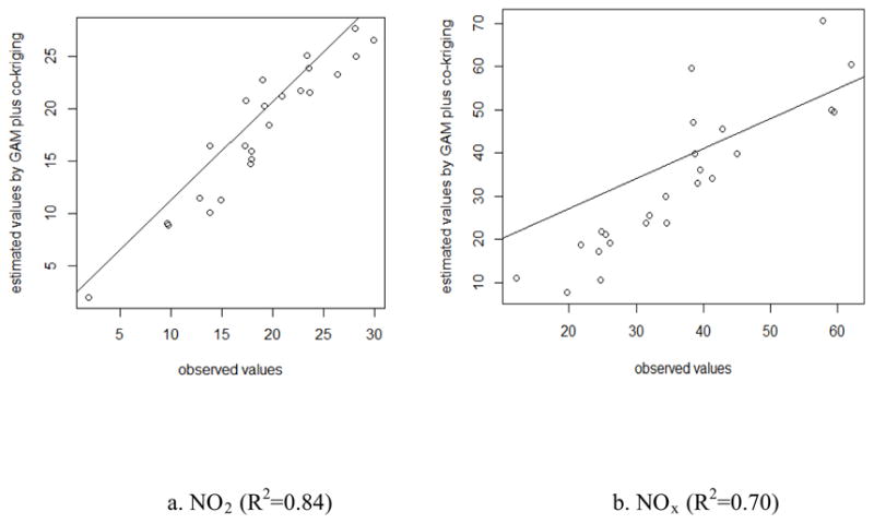
4.5. Comparison of modeled vs. observed long-term means

For long-term average concentrations, CV R² was 0.89 for NO₂ (RMSE =2.28) and 0.77 for NO_x (RMSE =6.8). Supplemental Materials Figure S8 shows the plots between predicted and observed long-term means for NO₂ and NO_x. Similar to our time-series predictions, we found that GAM plus cokriging improved R² by over 19% in variance (Table 2) for NO₂ and NO_x over linear regression to model spatially varying coefficients.

5. DISCUSSION

Our hierarchical two-stage models decomposed the spatiotemporal field into temporal components (temporal functions and their spatially-varying coefficients) at the first stage and then modeled the spatial fields of temporal components using a flexible spatial correlation structure at the second stage. Compared to a similar hierarchical modeling approach (Szpiro et al., (2010); Lindstrom et al., (2011)), our approach used the non-linear GAM to estimate spatial coefficients (β_i) of the temporal basis functions, incorporated regional residuals using cokrigging, and examined additional spatial covariates including long-term meteorology. The GAM provided a more flexible modeling framework than a linear model. For example, in our study, long-term average wind covariate contributed 21.2–34.5% of the β_i variability in GAM, but in the linear model it only accounted for about 8.0–10.0%.

Our model’s R² of 0.77 for the long-term average estimates of NO_x was slightly better than the reported R² (0.58–0.67) from the spatiotemporal models of NO_x for the similar Los Angeles region (Lindstrom et al., 2011; Szpiro et al., 2010). Given different sources of measurements, direct comparison is inappropriate although our approach outperformed the linear model by over 15% in variance explained based on our data. Our estimation of long-term NO₂ had a R² of 0.89, better than that for NO_x.

In this study, traffic-related variables (such as traffic flow or roadway length), land-use, meteorological or elevation factors had more or less influence on spatiotemporal variability of NO₂ and NO_x (Table 1, Figure 3 and Supplemental Materials Figure S2–S7). As expected, the shortest distance to roadways was negatively associated with the long-term averages (β₀), while the other traffic-related factors were positively associated. They together accounted for a large portion of variance. β₀ tended to be higher further away from the shorelines since the predominant wind in Los Angeles Basin blows from ocean to inland and wind carries emissions generated in the coastal and upwind regions to inland areas. These results were consistent with the conclusion in Szpiro et al. (2010) and Lindstrom et al. (2011). Among the meteorological factors, wind explained a large portion of variance on spatial variability of the temporal basis functions. Lower wind speed limited the dispersion of air pollutants, thus resulting higher long-term average β₀. Elevation was negatively associated with pollutant concentrations likely because of lower local emissions (e.g. a sparse roadway network) and stronger pollutant dispersion in hilly or mountainous areas. Since wind and elevation data are widely available in the U.S. (e.g. wind data from airport measurements, certain air monitoring station and other sources and elevation data from USGS), the exploration of such data in spatiotemporal modeling of air pollutant concentrations is recommended for epidemiological studies about acute or sub-chronic effects of air pollution. Further, since spatial autocorrelation contributed substantially to the estimation of spatial varying coefficients, spatial autocorrelation should not be neglected in similar modeling studies.

This study has several limitations. First, due to the unavailability of year-specific data, we used the 2003 roadway and 2005 AADT data to derive traffic-related covariates for 2006–2010. Although roadway and traffic data unlikely changed dramatically over the study region, these temporally-mismatched data may influence the performance of the models. Second, although we have examined the contribution of diesel truck emissions using Caltrans weigh-in-motion (WIM) data on freeways and highways, the fraction of diesel truck counts was not a statistically significant variable in any of the models. This is likely due to large uncertainties in the estimated truck count data since there were only five WIM stations in the study region (one in Orange County and four in Los Angeles). Third, the approach of splitting two continuous bi-week measurements to the four weekly estimates for the UCLA data may have introduced bias. The test using three different splitting methods (Supplemental Materials Table S5) showed limited influence of the interpolation methods on the prediction likely because of the small variation of concentration between two continuous weeks in our datasets. Ideally more than two time slices should be included whenever possible though. Fourth, the use of non-linear regression and residual spatial autocorrelation might cause an over-fitting problem. We tried to avoid overfitting by using cross validation, restricting the degree of freedom in the GAM and only incorporated non-linear covariates when necessary. Furthermore, the mgcv package in R used in our study controls the complexity of the splines by imposing the penalty on the parameters, lowering the over-fitting risk (Gill, 2001).

6. CONCLUSION

We used a hierarchical spatiotemporal model to combine routine time series with episodic measurements at a large number of locations to improve the estimation of spatiotemporal variability of NO₂ and NO_x concentrations in a dense urban area of southern California. Our model decomposed the spatiotemporal field of concentrations into the mean and residual. The mean was further decomposed into independent constant and varying temporal basis functions and local covariates were used to model spatially varying coefficients of the temporal basis functions with GAM plus cokriging. We found traffic, land-use and wind accounted for a large portion of the variance (beyond 35%) for the long-term average trend of concentrations. Spatial residuals accounted for a large portion of the variance of the temporal components (about 30% for NO₂ and 20% for NO_x). Leave-one-out cross validation produced an R² of 0.84 for NO₂ and 0.81 for NO_x when comparing the modeled weekly concentration with the observed trends at all routine monitoring stations. The approach has practical implication in studies of sub-chronic or short-term health effect that require high spatial and temporal resolutions of exposure.

Table 3.

Variogram Modeling of Spatial Residuals for β₀, β₁ and β₂

Statistics	NO2				NOx
	β0	β1	β2		β0	β1	β2
Model	Stable	Stable	Stable	Exponent	Stable	BesselK	Stable	Exponent
Parameter	0.3	0.2	0.2		0.5	2.19	0.2
Range	4.9 km	3.8 km	3.8 km	6.1 km	5.5 km	4.3 km	3.3 km	5.4 km
Partial sill	0.013	0.87	2.22	0.06	0.012	2.73	2.96	0.08

Table 4.

Comparison of our models with the linear model at 25 SCAQMD sites

Models	NO2			NOx
	CV R2 for time series	R2 for long-term averages	RMSE	CV R2 for time series	R2 for long-term averages	RMSE
N samples	5225	25	25	5225	25	25
Our model	0.82	0.84	2.46	0.75	0.70	6.4
Linear regression model	0.53	0.63	4.61	0.48	0.51	8.2

Highlights.

• Hierarchical spatiotemporal model predicted weekly NO₂ and NO_x concentrations well

• Episodic measurements supplemented routine time-series measurements in modeling

• Land-use, meteorology, and roadway were important in concentration prediction

References

- Cameletti M, Ignaccolo R. Comparing spatio-temporal hierarchical models for air quality data, Scientific Meeting of SIS. 45th Scientific meeting of Italian Statistical Society University of Padua.2010. [Google Scholar]
- Carslaw CD, Beevers DS, Tate EJ. Modeling and assessing trends in traffic-related emissions using a generalized additive model. Atmospheric Environment. 2007;41:5289–5299. [Google Scholar]
- Christakos G. A Bayesian maximum entropy view to the spatial estimation problem. Mathematical Geology. 1990;22:763–777. [Google Scholar]
- David P. Linear Algebra: A Modern Introduction. 2. Brooks/Cole; 2006. [Google Scholar]
- Finkenstadt B, Held L, Isham V. Statistical Methods for Spatio-Temporal Systems. Chapman & Hall/CRC; New York: 2007. [Google Scholar]
- Ghosh JK, Wilhelm M, Su J, Goldberg D, Cockburn M, Jerrett M, Ritz B. Assessing the influence of traffic related pollution on term LBW based on land use regression models and air toxics measures. American Journal of Epidemiology. 2012;175:1262–1274. doi: 10.1093/aje/kwr469. [DOI] [PMC free article] [PubMed] [Google Scholar]
- Gill J. Generalized Linear Models: A Unified Approach. Sage; Thousand Oaks, CA: 2001. [Google Scholar]
- Handelsman D. Optimal Power Transformations for Analysis of Sperm Concentration and Other Semen Variables. Journal of Andrology. 2002;23 [PubMed] [Google Scholar]
- Hart EJ, Yanosky DJ, Puett R, Ryan J, Dockery WD, Smith JT, Garshick E, Laden F. Spatial Modeling of PM10 and NO2in the Continental United States, 1985–2000. Environmental Health Perspectives. 2009;117:1690–1696. doi: 10.1289/ehp.0900840. [DOI] [PMC free article] [PubMed] [Google Scholar]
- Hoek G, Beelen R, Hoogh K, Vienneau D, Gulliver J, Fischer P, Briggs D. A review of land-use regression models to assess spatial variation of outdoor air pollution. Atmospheric Environment. 2008;42:7561–7578. [Google Scholar]
- Iglewicz B, Hoaglin CD. How to Detect and Handle Outliers. In: Mykytka FE, editor. The ASQ Basic References in Quality Control: Statistical Techniques. American Society for Quality; Milwaukee: 1993. [Google Scholar]
- Jerrett M, Arain A, Kanaroglou P, Beckerman B, Potoglou D, Sahsuvaroglu T, Morrison J, Giovis C. A review and evaluation of intraurban air pollution exposure models. Journal of Exposure Analysis and Environmental Epidemiology. 2005;15:185–204. doi: 10.1038/sj.jea.7500388. [DOI] [PubMed] [Google Scholar]
- Jerrett M, Burnett R, Pope A, Krewski D, Thurston G, Christakos G, Hughes E, Ross Z, Hi SY, Thun M. Spatiotemporal Analysis of Air Pollution and Mortality in California Based on the American Cancer Society Cohort: Final Report. State of Califonia Air Resources Board 2012 [Google Scholar]
- Li L, Wu J, Wilhelmc M, Ritz B. Use of generalized additive models and cokriging of spatial residuals to improve land-use regression estimates of nitrogen oxides in Southern California. Atmospheric Environment. 2012;55:220–228. doi: 10.1016/j.atmosenv.2012.03.035. [DOI] [PMC free article] [PubMed] [Google Scholar]
- Lindstrom J, Szpiro AA, Sampson DP, Sheppard L, Oron A, Richards M, Larson T. A flexible spatio-temporal model for air pollution: allowing for spatio-temporal covariates. UW Biostatistics Working Paper Series. 2011 doi: 10.1007/s10651-013-0261-4. [DOI] [PMC free article] [PubMed] [Google Scholar]
- Mahiyuddin W, Sahani M, Aripn R, Latif M, Thach T, Wong C. Short-term effects of daily air pollution on mortality. Atmospheric Environment. 2013;65:69–79. [Google Scholar]
- Ritz B, Wilhelm M. Ambient air pollution and adverse birth outcomes: methodologic issues in an emerging field. Basic & Clinical Pharmacology & Toxicology. 2008;102:182–190. doi: 10.1111/j.1742-7843.2007.00161.x. [DOI] [PMC free article] [PubMed] [Google Scholar]
- Szpiro AA, Sampson DP, Sheppard L, Lumley T, Adar DS, Kaufman DJ. Predicting intra-urban variation in air pollution concentrations with complex spatio-temporal dependencies. Environmetrics. 2010;21:606–631. doi: 10.1002/env.1014. [DOI] [PMC free article] [PubMed] [Google Scholar]
- Whitworth KW, Symanski E, Lai2 D, Coker LA. Kriged and modeled ambient air levels of benzene in an urban environment: an exposure assessment study. Environmental Health. 2011;10:21. doi: 10.1186/1476-069X-10-21. [DOI] [PMC free article] [PubMed] [Google Scholar]
- Wood SN, Augustin NH. GAMs with integrated model selection using penalized regression splines and applications to environmental modelling. Ecological Modelling. 2002;157:157–177. [Google Scholar]
- Wu J, Wilhelm M, Chung J, Ritz B. Comparing exposure assessment methods for traffic-related air pollution in an adverse pregnancy outcome study. Environmental Research. 2011;111:685–692. doi: 10.1016/j.envres.2011.03.008. [DOI] [PMC free article] [PubMed] [Google Scholar]
- Yu H, Chen J, Christakos G, Jerrett M. BME estimation of residential exposure to ambient PM10 and ozone at multiple time scales. Environmental Health Perspectives. 2009;117:537–544. doi: 10.1289/ehp.0800089. [DOI] [PMC free article] [PubMed] [Google Scholar]
- Zanobetti A, Schwartz J, Samoli E, Gryparis A, Touloumi G, Peacock J, Anderson HR, Tertre LA, Bobros J, Celko M, Goren A, Forsberg B, Michelozzi P, Rabczenko D, Hoyos PS, Wichmann EH, Katsouyanni K. The temporal pattern of respiratory and heart disease mortability in response to air pollution. Environental Health Perspective. 2003;111:1188–1193. doi: 10.1289/ehp.5712. [DOI] [PMC free article] [PubMed] [Google Scholar]
Associated Data
This section collects any data citations, data availability statements, or supplementary materials included in this article.