


Abstract
RIP-seq has recently been developed to discover genome-wide RNA transcripts that interact with a protein or protein complex. RIP-seq is similar to both RNA-seq and ChIP-seq, but presents unique properties and challenges. Currently, no statistical tool is dedicated to RIP-seq analysis. We developed RIPSeeker (http://www.bioconductor.org/packages/2.12/bioc/html/RIPSeeker.html), a free open-source Bioconductor/R package for de novo RIP peak predictions based on HMM. To demonstrate the utility of the software package, we applied RIPSeeker and six other published programs to three independent RIP-seq datasets and two PAR-CLIP datasets corresponding to six distinct RNA-binding proteins. Based on receiver operating curves, RIPSeeker demonstrates superior sensitivity and specificity in discriminating high-confidence peaks that are consistently agreed on among a majority of the comparison methods, and dominated 9 of the 12 evaluations, averaging 80% area under the curve. The peaks from RIPSeeker are further confirmed based on their significant enrichment for biologically meaningful genomic elements, published sequence motifs and association with canonical transcripts known to interact with the proteins examined. While RIPSeeker is specifically tailored for RIP-seq data analysis, it also provides a suite of bioinformatics tools integrated within a self-contained software package comprehensively addressing issues ranging from post-alignments’ processing to visualization and annotation.
INTRODUCTION
Comprehensive transcriptome analyses suggest that only 1–2% of the human or mouse genome is protein coding, whereas 70–90% is transcriptionally active, but do not code for proteins, and thus denoted as non-coding RNA (ncRNA) (1). Based on the loci of origin, the ncRNAs can arise from literally anywhere in the genome (reviewed in (2)). The lengths of these ncRNAs are extremely diverse, ranging from 100 nucleotides (nt) to >100 kb (not considering small ncRNA such as microRNA). The ncRNAs longer than 200 nt are commonly referred to as long ncRNA (lncRNA). Mounting evidence suggests that many of these lncRNAs are evolutionarily conserved, functionally interacting with chromatin regulators and participating in gene regulation (3–5). The protein–RNA regulatory complexes are referred to as ribonucleoprotein (RNP). For instance, the chromatin regulator polycomb repressive complex 2 (PRC2) is responsible for histone 3 lysine 27 tri-methylation (H3K27me3), which is linked to global gene silencing (6). Several lncRNAs such as HOTAIR, Xist and Kcnq1ot1 bind to and target PRC2 to silence specific gene clusters. This RNA-mediated gene regulation has been shown to be crucial for embryonic development, cell differentiation and tumor suppression (7).
As another example, P-TEFb (positive transcription elongation factor b) is a protein complex that comprises cyclin-dependent kinase 9 (CDK9) and a cyclin (T1 or T2) (CCNT1 or 2) (8). P-TEFb phosphorylates (through CDK9) RNA polymerase II (RNAP II) carboxyl-terminal domain to initiate or restore transcription elongation in human cells. However, binding of a small nuclear RNP (snRNP) containing a ∼330-nt ncRNA 7SK or RN7SK (chr6:52,860,418–52,860,749) to the P-TEFb subunit CCNT1 associates with inhibition of the kinase activity. The inhibitory RN7SK snRNP can be competitively displaced by the nascent TAR (transactivation response) HIV RNA bound with the Tat viral protein, activating P-TEFb kinase and transcriptional elongation (9). In other words, the association between P-TEFb and RN7SK-snRNP competes with TAR-Tat for binding to CCNT1, which may dictate efficient synthesis of viral transcripts (8).
Despite tremendous efforts, our knowledge of ncRNAs and their functions is still limited, which is largely due to the lack of a systematic experimental approach. Recently, RNP immunoprecipitation (IP) followed by high-throughput sequencing (HTS) (RIP-seq) has been developed to capture genome-wide RNA transcripts that physically interact with proteins or protein complexes (4). RIP-seq is conceptually parallel to ChIP-seq (chromatin IP followed by HTS), which is designed to identify TF binding sites (TFBS) or histone modification patterns at the genome scale (6). Both protocols use antibody to specifically pull-down a protein of interest from cell extracts and generate sequence reads associated with that protein. A control dataset is usually generated either by sequencing mutant depleted of the protein of interest, a library generated with non-specific antibody such as IgG, or RNA/DNA input library. In ChIP-seq, fragments (200–600 bp) of the protein-bound DNA are sequenced from the 5′ end on both strands. In principle, the double-strandedness of the bound DNA entails strand-dependent bi-modality (10). This property is widely exploited by many popular ChIP-seq algorithms such as MACS (11) and QuEST (12) (Table 1) in genome-wide search of bona fide TFBS.
Table 1.
Comparison programs for RIP-seq or PAR-CLIP analysis
| Methods | Reference | Specialization | Implementation | Version | Strand-specific scoring | False discovery rate | Compare with control fit | Statistical model |
|---|---|---|---|---|---|---|---|---|
| MACS | (11) | ChIP-seq | Python | 1.4.1 | No | Yes | Yes | Local Poisson |
| QuEST | (12) | ChIP-seq | Perl/C++ | 2.4 | No | Yes | Yes | Kernela |
| HPeak | (20) | ChIP-seq | Perl | 3 | No | No | No | HMMb |
| Cuffdiff | (15,16) | RNA-seq | C++ | 1.3.0 | Yes | Yes | Yes | Cufflinks + Differential Testc |
| PARalyzerd | (35) | PAR-CLIP | Java | 1.0.0 | Yes | Yes | No | Kernela |
| Rule-basede | (4) | RNA-seq | R | 0.99.0 | Yes | No | No | FC and RPKMf |
| RIPSeeker | Proposed | RIP-seq | R | 0.99.0 | Yes | Yes | Yes | HMMg |
aGaussian kernel smoothing.
bTwo-state HMM using Viterbi with generalized and zero-inflated Poisson emissions.
cDe novo transcript assembly using Cufflinks followed by differential test based on beta negative binomial distribution using Cuffdiff.
dSpecialized in PAR-CLIP data by taking into account both the read counts and  conversion.
eImplemented as a built-in function in RIPSeeker.
fFold change and RPKM thresholding on annotated transcripts (default: FC ≥3; RPKM ≥0.4).
gTwo-state HMM using forward–backward with NB emission followed by RIP detection using Viterbi and log odd posteriors.
Although RIP-seq experiments share similarities with ChIP-seq and RNA-seq, it has a fundamentally different goal: discovery of protein-associated RNA transcripts. Several distinct properties and challenges need to be addressed in RIP-seq data analysis. Figure 1 illustrates the following comparison between the three sequencing platforms. First, because of the splicing events that commonly occur in mammalian cells, RNA reads from RIP-seq need to be aligned to the reference genome using a spliced aligner such as TopHat (13). For the same reason, the aligned RNA reads should not be extended further along the genome, as commonly practiced by most ChIP-seq analyses to increase detection power. Second, as RNA molecules are single-stranded, the bimodal property observed in ChIP-seq for double-stranded DNA does not hold for RIP-seq. Consequently, the peak callers that are designed to look for ‘twin peaks’ separated by a distance depending on the cDNA fragment length do not apply to RIP-seq analysis (Supplementary Figure S3). Moreover, to detect strand-specific RNA such as Kcnq1ot1 (an antisense transcript overlapping the coding gene Kcnq1), read counts on each strand needs to be modeled separately. Third, TFBS of DNA is usually enriched for some consensus DNA sequence motifs. RNA molecules, on the other hand, are likely to interact with proteins through secondary or even tertiary structure (e.g. repA stem loop of Xist) (7). Thus, there might not be explicit primary RNA sequence motif that can be identified directly by multiple sequence alignments. Finally, RIP-seq aims at finding the entire transcripts rather than punctuate binding sites, as in ChIP-seq or PAR-CLIP (Photoactivatable-Ribonucleoside-Enhanced Crosslinking and Immunoprecipitation), which is another protocol designed to specifically detect direct RNA–protein interaction sites (14). A suitable RIP-seq ‘peak caller’ needs to be adaptive to a wider and more flexible range of regions due to various lengths of the RNA transcripts. These fundamental differences render many ChIP-seq algorithms unsuitable for RIP-seq analysis.
Figure 1.

Simplified biological principles of (a) ChIP-seq, (b) RNA-seq and (c) RIP-seq. In ChIP-seq (a), double-stranded DNA bound with protein of interest is pulled-down by an antibody, followed by HTS. Because the reads are usually shorter than the double-stranded DNA fragment, a true binding site gives rise to symmetrical peaks observed on the + and − strand separated by the distance approximately the same as the length of the fragment. However, the same principle does not apply to (b) RNA-seq and (c) RIP-seq because the RNA transcripts are single-stranded. On the other hand, noise or missing reads due to imperfect immunoprecipitation and non-specific protein–RNA interaction are intrinsically unique to RIP-seq.
Furthermore, programs for de novo transcript assembly followed by differential expression (DE) analysis, such as the Cufflinks/Cuffdiff suite (15,16), and for DE on a set of known transcripts, such as DESeq (17), may appear applicable to RIP-seq analysis. Unlike peak-calling strategy, however, the transcript-based methods assume the full transcriptome being sequenced at a fairly deep coverage (as usually the case in RNA-seq) and thus may be sensitive to background noise typical to the IP-based protocols, which is due to both the non-specific RNA interactions with a protein of interest and the non-specific RNA input from the pull-down of the (mutant) control (Supplementary Figures S3 and S4).
Therefore, an effective approach for RIP-seq analysis should (1) effectively model the distributions of reads that arise from bona fide protein–RNA interactions under considerable noise and (2) infer RIP regions taking into account the adjacent regions. The aforementioned considerations will lead to a robust model, which is tolerant to missing values and is discriminative between noise and true signals.
MATERIALS AND METHODS
RIPSeeker overview
To address the aforementioned RIP-seq specific issues, we propose a novel statistical framework implemented as an R software package called RIPSeeker. RIPSeeker provides a comprehensive analytical suite for RIP-seq analysis, not only including predicting RIP regions with or without a control library but also processing alignments, automatic genomic annotation, visualization from UCSC browser, etc. Figures 2 and 3 depict the core idea and more detailed workflow of RIPSeeker, respectively. Each computational step depicted in oval shape in Figure 3 is detailed in the corresponding subsections later. The input for RIPSeeker is a list of read alignments in BAM/BED/SAM format. Mapping reads to the reference genome can be performed by any RNA-seq aligner, such as TopHat (13). After post-processing the alignment input (detailed in the next section), RIPSeeker first stratifies the genome into non-overlapping bins of automatically selected (Automatic bin size selection) or a fixed user-defined size. Each bin may contain more than one aligned read. Multiple bins may together correspond to a single RNA transcript that binds to the protein of interest. Thus, these bins when treated as individual observations are not independent identically distributed (i.i.d.) and need to be treated as dependent events. Hidden Markov model (HMM) provides a sensible and efficient way to probabilistically model the dependence between sequential events through hidden variables (18,19). The adaptation of HMM is inspired by HPeak, which was specifically designed for ChIP-seq (20).
Figure 2.

The core idea of RIPSeeker. After IP and HTS, reads are aligned to the reference genome and tallied within non-overlapping bins of size determined automatically for each specific chromosome based on the coverage and chromosome length. Considering the read count in each bin as observed data point, a two-state hidden Markov model with negative binomial (NB) emission is used to infer the RIP bins (assumed to be) associated with the hidden state corresponding to the NB with the larger mean. The inference step yields both the posterior probability of RIP state and the optimized HMM parameters. Next, Viterbi algorithm is applied to derive the most probable hidden state sequence, with 1 denoted as the background state and 2 as the RIP state. The merged adjacent RIP bins are subject to significance tests based on the posterior probabilities for the background and enriched states.
Figure 3.

Detailed workflow of RIPSeeker. RIPSeeker processes the input alignment files in BAM/BED/SAM format and determines the bin size based on the unique read counts on each chromosome. The two-state HMM parameters are initialized by negative binomial (NB) mixture model and optimized through EM. The two hidden states presumably correspond to the background and RIP regions. Optionally, each multihit is assigned to a unique locus with the highest posterior probability for the RIP state among other loci (mapped by the same read). The HMM parameters are then re-estimated with the augmented read count data. Viterbi algorithm running on the optimized HMM parameters yields the maximum likelihood hidden state sequence across each chromosome. The (merged) RIP regions from the Viterbi predictions are further filtered by the statistical tests for the model confidence based on the posterior encodings. Finally, annotated RIP regions are exported and programmatically uploaded to UCSC browser for visualization.
As an overview, RIPSeeker consists of two major steps: probabilistic inference of RIP regions (HMM posterior decoding and parameter optimization) and significance test for the inferred RIP regions from HMM (Detect RIP regions). In the first step, we apply a two-state HMM to model the background and RIP distributions (or emission probabilities) of RIP-seq read counts as negative binomial (NB) distributions, which has been shown by Anders and Huber (17) to be a more realistic parametric model than Gaussian and Poisson models (detailed in Supplementary Methods Section Negative binomial distribution). The parameters of HMM are learned from the data by expectation-maximization (EM). The intermediate quantities required in the EM iterations are efficiently computed using forward–backward algorithm. After the optimization, Viterbi algorithm is applied to derive the most probable sequence of hidden states, which encodes whether each region is background (1) or RIP (2) in the genome (Figure 2). The consecutive RIP bins are merged into a single RIP region. In the second step, we compute the statistical significance of each RIP region with or without a control library based on the posterior probabilities derived directly from the HMM.
RIPSeeker is able to detect strand-specific RIP regions by running the same workflow on either plus and minus strand separately, making use of the strand-specific information retained in the original RIP-seq protocol (4,21). In addition, RIPSeeker takes advantage of modern computational architecture equipped with multiple processors by treating each chromosome as an independent thread and computing multiple threads in parallel using mclapply from parallel R package. Thus, the most time-consuming step such as HMM inference operates on per-chromosome basis, with each running on a separate CPU core. The parallel computing is much more computationally and memory efficient than computing the entire genome all at once by treating it as a single concatenated sequence. RIPSeeker has numerous other features, including disambiguating multihits (i.e. reads mapped to multiple loci), automatic annotation of RIP regions, gene ontology (GO) enrichment analysis, and UCSC visualization. All of these features are detailed in the following subsections.
Processing alignment inputs
Unlike many existing peak-calling software, RIPSeeker does not simply import the alignments, but rather uses series of preprocessing procedures to address common problems inherent to high-throughput sequencing data as follows. Given a BAM/SAM/BED file, RIPSeeker by default removes duplicate reads and flags multihits. Duplicate reads are a set of reads that align to exactly the same genomic coordinate. Because transcripts are usually hundreds or thousands of nucleotides long, and thus much longer than the read (25–100 nt), chances of the same 25–100-nt portion of the transcript being sequenced multiple times at exactly the same coordinate are small and may likely be due to PCR artifact. Multihits represent multiple alignments of the same read due to gene duplications or repetitive elements in the genome. Rather than removing those multihits, which typically constitute a substantial proportion of the total mapped reads, RIPSeeker (by default) flags them but does not use them for the initial training of HMM and in the later step, assigns each of these reads to a unique region [Disambiguate multihits using posterior decoding from HMM (optional)] and then re-trains the HMM with augmented data of unique read counts.
If multiple alignment files are provided as technical replicates for RIP or control sample, RIPSeeker first applies the aforementioned procedure to each alignment file and then merges the preprocessed alignments. The output in this step is an alignment object belonging to GappedAlignments class defined in the GenomicRanges library (22). The extensive use of the existing classes in the popular GenomicRanges library allows RIPSeeker to be easily incorporated into a custom computational workflow constituting various other established Bioconductor packages. Like ChIP-seq, a control library representing background and non-specific binding events is important in RIP-seq analysis to filter out false-positives. Accordingly, a control library is supported as an optional (but not mandatory) parameter to RIPSeeker. The control alignment file is distinguished from RIP library by a user-supplied keyword in the main ripSeek function; e.g., ripseek(bamPath = bamfiles, cNAME = ‘CTL’) for ‘lib_RIP.bam’ and ‘lib_CTL.bam’ as RIP and control alignment inputs, respectively.
Finally, RIPSeeker supports paired-end alignments. Briefly, paired-end alignment files are read in through readGappedAlignmentPairs from GenomicRanges. RIPSeeker then combines properly paired reads into a single alignment record, making use of the CIGAR flag ‘N’ to indicate the number of bases between the mate pairs (i.e. the length of the insert fragment). In other words, the paired-end alignments are treated as gapped alignments of long fragments. After converting the GappedAlignmentPairs object into GappedAlignments object, the alignments’ processing proceeds as described previously.
Automatic bin size selection
Based on the preprocessed alignments for a chromosome, RIPSeeker divides the chromosome into non-overlapping bins of equal size b and computes the number of reads that fall into each bin, where b needs to be determined either empirically (e.g. based on the gel-selected length of the RNA fragment) or computationally. If the bin size is too small, the read counts fluctuate greatly, making it difficult to discern the underlying read count distribution. Additionally, input size to HMM increases as bin size decreases. A small bin size incurs a long Markov chain of read counts to model, making the computation inefficient. On the other hand, if a bin size is too large, resolution becomes poor. Consequently, one cannot detect the local RIP region with subtle, but intrinsic, difference from the background, and the RIP regions tend to be too wide for designing specific primer for validation.
Intuitively, selecting an appropriate bin size for each chromosome is analogous to choosing an optimal interval for building a histogram (23). Here we implement the algorithm developed by Shimazaki and Shinomoto (2007) (24), which is based on the goodness-of-the-fit of the time histogram to estimate the rate of neural response of an animal to certain stimuli in a spike-in experiment. This approach has been successfully applied in a recently developed ChIP-seq program (23). Algorithm 1 describes the pseudocode adapted from (24) that iteratively estimates the cost C of increasing bin size b within a defined range [default: (minBinSize = 200 nt, maxBinSize = 1200 nt) with 5-nt increment] and finally selects the  with minimum cost. The default range was used in the tests to achieve efficient computation and reflect the fragment size or the band (200–1200 nt) selected from the gel electrophoresis in the RIP-seq library construction (4). Notably, consecutive RIP bins are merged, leading to a wider RIP region (Detect RIP regions).
Algorithm 1: AutomaticBinSizeSelection.
for
 do
do
Divide chromosome sequence into N bins of width b.
Count number of read counts xi that enter the i’th bin.
Compute:  and
and 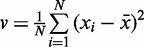 .
.
Compute: 
end for
Choose  that minimizes C(b).
Bin count
Based on the defined bin size, the number of reads that fall within each bin is computed using function countOverlaps from IRanges package (25). The output is a one-dimensional vector of integers sorted by the chromosomal coordinates.
NB mixture model initialization
Because the EM algorithm in HMM tends to fall into local optimum with poor initialization, NB mixture model with two mixture components (2-NBM) is first applied to the data to obtain a reasonable estimate for the HMM parameters. Essentially, one can think of 2-NBM as a special case of two-state HMM with two distinct NB emission distributions: the 2-NBM assumes that the data points are not identically distributed but sampled independently from a mixture of two NB distributions, whereas the two-state HMM is a more general framework for non-i.i.d data (addressing both mixture distribution and dependence between data points).
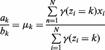
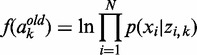
Given a 2-NBM, the goal is to maximize the likelihood function with respect to the parameters comprising ak and bk for the two NB components (thus  ) and the mixing coefficients
  , which are the priors
  . The maximum likelihood (ML) estimators of aforementioned are:
 |
(1) |
 |
(2) |
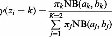
where  (commonly referred to as responsibility) denotes the posterior probability
  and N is the total number of bins. Because there is no analytical solution for the aforementioned system equation, a modified EM procedures called ECM (Expectation Conditional Maximization) is used (19,26):
For
 and
and  corresponding, respectively, to the background and RIP NB distributions, initialize the
  as
as  (i.e. the second-last and last quantiles of the non-zero read counts),
  as {1,1} and
 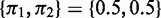 .
.- E step: Evaluate
 for each bin (
 ) using the current parameter values:
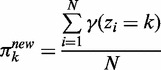
(3) - M step: Re-estimate the mixing proportion using the current responsibility based on (2):
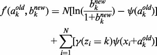
(4) - CM step: As we cannot evaluate ak and bk simultaneously, we turn to a variation of the M-step called conditional maximization (26), where we fix variable ak to evaluate bk using (1), and then use Newton’s method to update ak:
where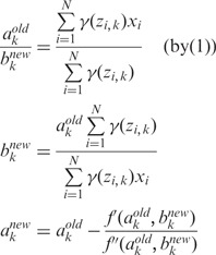
(5)  is the logarithmic posterior probability of the data
  , which is the product of the conditional probabilities based on the conditional independence assumption;
  and
and  are, respectively, the first and second derivatives of f with respect to ak:
(6) 
(7)
where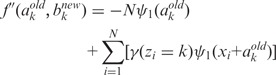
(8)  and
and  are the di and trigamma function, which are the first and second derivative of the logarithmic gamma function computed by the R built-in functions digamma and trigamma.
 - Evaluate the log likelihood:
If the fraction of increase for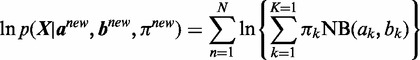
(9) 
 (9) is less than a threshold (default: 0.01) comparing with
  from the previous iteration, then stop; otherwise repeat step 2–4.
HMM posterior decoding and parameter optimization
The two-state HMM is similar to the 2-NBM, except that  in the E step (3) is computed using forward–backward algorithm, taking into account the dependence between consecutive latent variables in the hidden Markov chain:
| (10) |
where
| (11) |
| (12) |
The M step computes an additional ML estimator for the transition probability:
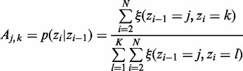 |
(13) |
where
 |
(14) |
The CM step is the same as in 2-NBM. For a more detailed description of the two-state HMM, readers are referred to Section Negative Binomial Hidden Markov Model in the Supplementary Methods or the more general framework described in (18). The two-state HMM generally performs better than NBM on simulated count data with known hidden states and transition probabilities. HMM with NBM initialization in turn performs better than HMM alone (Supplementary Figure S1). Some ideas on the HMM R implementation are adopted from the MatLab functions (http://perso.telecom-paristech.fr/ cappe/Code/H2m/).
Disambiguate multihits using posterior decoding from HMM (optional)
Each multihit (i.e. read aligned to multiple loci) flagged in the preprocessing step is assigned to a unique locus corresponding to the jth bin with the highest posterior or responsibility from the RIP state (Figure 4). Intuitively, the RIP state corresponds to the read-enriched loci. Disambiguating multihits in this way will potentially improve the power of detecting more RIP regions, but may also introduce certain bias toward the idea of ‘rich gets richer’. Thus, this step is optional and controlled by the parameter assignMulthits in the main function ripSeek (described in the manual and vignette). After this step, RIPSeeker will rerun the steps from Automatic bin size selection to HMM posterior decoding and parameter optimization to improve the model estimation with augmented read count data. Optionally, user can choose not to reiterate the training process to go straight to the next step to detect RIP regions.
Figure 4.

Disambiguating multihits based on posterior decodings from HMM. Given more than one valid aligned loci on the same or different chromosome (x-axis), the multihit read is assigned to the locus with the highest posterior probability (y-axis) for the second state  associated with the
  with the larger mean
  .
.
Viterbi prediction of enriched bins
After learning the model parameters of HMM (and disambiguating the multihits), we can obtain the sequence of hidden states for  latent variables that maximizes the log joint likelihood
 using Viterbi algorithm based on dynamic programming (18) (detailed in Supplementary Methods Section Viterbi algorithm).
Detect RIP regions
To assess the statistical significance of the RIP predictions, we assign each bin a RIPScore:
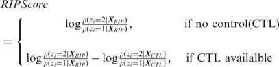 |
(15) |
If control library is unavailable, the RIPScore is the log odds ratio of the posterior for the RIP state ( ) over the posterior for the background state (
 ); otherwise, the RIPScore is the difference between the RIPScores evaluated separately for RIP and control libraries. The scoring system (15) captures the model confidence for the RIP state of each bin in the RIP library penalized by the false confidence for the ‘RIP’ state of the same bin in the control library. In addition, RIPScore obviates scaling of read counts. As sequencing depth usually differs between RIP and control libraries, scaling is necessary if the statistical score was derived from the read count differences, such as in MACS (11). However, simplistic linear scaling may distort the data. This issue is effectively avoided by RIPSeeker through the elegant use of posteriors (15).
The consecutive RIP bins predicted in the aforementioned Viterbi step are merged into a single RIP region. An aggregate RIPScore as the averaged RIPScores (15) over the merged bins is assigned to each RIP region. To assess the statistical significance of the RIPScore for each region, we assume (and indeed observe in Supplementary Figure S2) that the RIPScore approximately follows a Gaussian distribution with mean ( ) and standard deviation (
 ) estimated using the RIPScores over all of the bins. The rationale is based on the assumption that most of the RIPScores correspond to the background state and together contribute to a stable estimate of the test statistics (TS) and P-value:
| (16) |
| (17) |
To correct for multiple testing, the standard Benjamini–Hochberg method is used (27) with the R built-in function p.adjust to compute the q-value.
In addition, if control is available, an empirical false discovery rate (eFDR) is estimated based on the idea of ‘sample swap’ inspired by MACS (11). Briefly, at each P-value, RIPSeeker finds the RIP regions over control (CTL) and control regions over RIP. The eFDR is defined as the number of ‘RIP’ (false-positive) regions identified from CTL-RIP comparison over the number of RIP regions from the RIP-CTL comparison:
| (18) |
The maximum value for eFDR is 1 and minimum value for eFDR is max(P-value, 0). The former takes care of the (rare) occasion when the numerator is bigger than the denominator in (18), and the latter for zero numerator.
Genomic visualization
To make RIP-seq analysis more intuitive, RIPSeeker provides a function viewRIP, which launches online UCSC genome browser with programmatically uploaded custom track corresponding to the loci of RIP regions and scores [RIPScore, −log10(P-value), −log10(q-value), −log10(eFDR)] generated from the aforementioned RIP regions detection. This task is accomplished seamlessly within the R console by making use of the available functions from rtracklayer (28).
Genomic annotation and GO enrichment analysis
Given the genomic coordinates of each predicted RIP region, RIPSeeker queries the Ensembl database whether each region is nearby or overlaps any gene annotation (including known ncRNAs). To access the up-to-date Ensembl database, RIPSeeker uses useMart and getAnnotation from biomaRt and ChIPpeakAnno Bioconductor packages to dynamically establish Internet connection to the database and retrieve the up-to-date (or archived) annotations (29–31). Subsequently, annotatePeakInBatch and getEnrichedGO from ChIPpeakAnno (Bioconductor) (31) are used to efficiently annotate all of the predicted regions and reports (if any) enriched GO terms, respectively. A predicted RIP region may overlap multiple known genes, all of which will be reported as separate records.
RIPSeeker outputs
The final outputs of RIPSeeker consist of five useful files: (1) a tab-delimited text file containing the statistics from the previous section, genomic coordinates, spatial information relative to the neighbor gene, gene symbol and description for the gene; (2) and (3) the same information in General Feature Format with and/or without gene annotations; (4) enriched GO in tab-delimited file; (5) all intermediate and final results saved in RData that can be imported directly into the R console by the load command. File (1) provides the most detailed information directly viewable in Excel. Files (2) and (3) can be imported to a dedicated genome browser such as Integrative Genomic Viewer (32) to visualize and interact with the putative RIP regions with scores.
Combining biological replicates
In RIP-seq experiments, biological replicates are important, as they can increase detection power and further filter out false-positives due to substantial background noise. Thus, we provide a helper function combineRIP to facilitate user to intersect, merge or pool peaks in the General Feature Format files generated previously.
Rule-based method
Furthermore, we implemented computeRPKM and rulebaseRIPSeek as built-in functions in RIPSeeker by following the original rule-based methods devised in (33) and (4), respectively. The function rulebaseRIPSeek serves both as a (baseline) comparison method (see later) and a reasonable supplementary option for the RIPSeeker user to query known genes’ or transcripts’ (relative) abundance (in two conditions). Briefly, transcriptome annotation for a given species is dynamically retrieved from Ensembl or UCSC database using makeTranscriptDbFromBiomart or makeTranscriptDbFromUCSC from R package GenomicFeatures, respectively (34). Given a list of alignment datasets (BAM) (preprocessed by RIPSeeker) for RIP and/or control libraries, the expression of each annotated transcript is computed by computeRPKM as ‘reads per kilobase of exon per million mapped reads’ (RPKM). To compute read counts, computeRPKM uses the function summarizeOverlaps from GenomicRanges (22). A transcript is predicted as the protein interaction partner if its RPKM expression and the ratio of RPKM[RIP]/RPKM[control] (on either + or − strand) are above t1 and t2. By default,  and
and  , consistent with the thresholds applied in the original study (4). Pertinent to the data, Ensembl annotation version 65 and 69 are used for NCBIM37/mm9 mouse and GRCh37/hg19 human genome assemblies, respectively.
Comparison with published methods
To compare RIPSeeker with other algorithms popular in various high-throughput sequencing analyses, we attempted to choose the best alternative approaches despite that they were not specialized for RIP-seq analysis (Table 1). Specifically, we chose three ChIP-seq algorithms, including MACS, QuEST and HPeak; two RNA-seq algorithms Cufflinks + Cuffdiff and Rulebased and one PAR-CLIP algorithm PARalyzer. Except for explicitly mentioned, default cutoffs were used for each algorithm. The specific settings for the aforementioned programs are described in Supplementary Methods. The cutoff for RIPSeeker’s predictions is set to eFDR ≤0.1 OR q-value ≤0.1 for the following tests.
ChIP-seq programs
MACS and QuEST represent parametric and non-parametric frameworks based on local Poisson model and Gaussian kernel density estimation, respectively. HPeak also uses a two-state HMM but differs from RIPSeeker in many technical aspects. In particular, HPeak assumes that read counts from ChIP and background, respectively, follow generalized Poisson and zero inflated Poisson distributions and directly uses the Viterbi algorithm to train the HMM. In contrast, RIPSeeker performs the exact inference through forward–backward algorithm (10), followed by Viterbi prediction, assuming distinct NB emission probabilities for RIP and background. In addition, HPeak identifies ChIP region using generalized Poisson posterior probabilities, whereas RIPSeeker uses log odd posterior (15) to derive (adjusted) P-value (17) and eFDR (18). Unlike RIPSeeker, none of the three ChIP-seq algorithms have an option to identify strand-specific peaks. To make fair comparison when strand-specific sequencing data were used, alignments on ‘+’ and ‘−’ strands were extracted from the total alignments and provided as separate inputs to the three peak callers. The peaks from the same program were then pooled together to represent its predictions.
RNA-seq program
The RNA-seq software suite Cufflinks (15) was applied to RIP-seq data, attempting to assemble de novo transcripts from the alignments and compare their expression level in RIP with control library using Cuffdiff. For brevity, the Cufflinks + Cuffdiff approach is referred to as Cuffdiff from now on. In addition, we included the Rule-based method, also commonly used in RNA-seq analyses (Section Rule-based method) as the baseline comparison method.
PAR-CLIP program
PARalyzer is a recently developed program specifically tailored for PAR-CLIP analysis (35). As PARalyzer is the only other package that is designed for IP-based RNA-seq data, it is highly relevant to compare it with RIPSeeker. Besides read counts, PARalyzer uses the thymine to cytosine conversion ( ) induced by cross-linking between the RNA-binding protein and its target (14). However, the requirement for such induced mutation in the sequencing data makes PARalyzer incomparable with other peak callers on RIP-seq data. Conversely, however, RIPSeeker, MACS and HPeak, which do not require an external control library, are in fact applicable to PAR-CLIP data. Indeed, the authors of PARalyzer show that the number of observed
  conversions strongly correlates with the total number of reads (addition file 1 from (35)). Accordingly, we applied RIPSeeker, MACS, HPeak and PARalyzer to the PAR-CLIP datasets. The former three only exploit the read count information, and the latter exploits both the read counts and the
  conversions. Because no external control library was used in the PAR-CLIP experiments, RIPSeeker, MACS and HPeak will infer peaks solely based on enrichment relative to the implicit background internal to the PAR-CLIP library. Notably, such comparison may also indirectly examine the importance of the conversion information on top of the single-nucleotide resolution it provides.
Union of peaks
To facilitate some of the following comparisons, the peaks or transcripts identified from multiple biological replicates were pooled (and merged). No pooling is needed for Cuffdiff because it uses biological replicates to estimate the variance and outputs a single set of transcripts (16). Thus, each method has a single representative set of predictions for the same dataset. Union rather than intersection among biological replicates was chosen to maximize sensitivity, as we found that the same algorithm performed differently on biological replicates, perhaps due to background noise and sequencing depths. For convenience, the ChIP-seq algorithms and RIPSeeker are sometimes referred to as ‘peak callers’ and the Cuffdiff and Rule-based methods as ‘transcript-based’ methods. Notably, we use the term ‘peak callers’ for any method that predicts de novo regions mostly smaller than the whole transcript, even though the ‘peaks’ in some cases are large ‘regions’.
Receiver operating curve
To examine the sensitivity and specificity of each method, we need a set of ‘gold-standard’ RNA-binding sites for the proteins of interest, which is currently unavailable. To still conduct a similar systematic test, we define the ‘gold-standard’ as a set of peaks consistently ‘agreed’ on by the majority (>50%) of the tested programs on the same dataset. Different peaks from two methods ‘agree’ if they overlap each other or are within 1000 nt distance. To benchmark each method, the number of positive peaks P is defined as the number of predictions that overlap with the ‘gold-standard’ peaks. Similarly, the number of negative peaks N is defined as the number of predictions that do not overlap with the ‘gold-standard’ peaks. Given a set of peaks that pass the cutoff according to the program-specific scoring system (described later), the number of ‘true positive peaks’ TP (‘false positive peaks’ FP) is defined as the number of peaks that (do not) belong to the positive peak list. Finally, we define the ‘true positive rate’  and the ‘false positive rate’
  . The receiver operating curve (ROC) is plotted by iteratively evaluating TPR (y-axis) and FPR (x-axis) based on an increasing cutoff of the program-specific score. TP and FP at each cutoff are computed using the function prediction from R package ROCR, and the TPR and FPR are subsequently calculated using function performance from the same package.
Except if mentioned otherwise, the program-specific scoring systems used to construct the ROC are as follows: for MACS, −10log10(P-value) (i.e. fifth column of the peaks.bed output); for HPeak, the absolute normalized cumulative log-transformed posterior probability (i.e. the last column of the all.regions.txt output); for QuEST, the normalized enrichment fold at the maximum position within the region (i.e. fifth column in the output file ChIP_calls.filtered.bed); for Cuffdiff, −log10(P-value) in isoform_exp.diff; for PARalyzer, ModeScore [score of the highest signal / (signal + background) value] in output file named cluster; for Published peaks from the ENCODE data, −log10(P-value); for Rulebased, fold-change of RPKM in RIP over control; for RIPSeeker, −log10(P-value) (17).
RIP-seq library construction for CCNT1
As a further proof-of-concept, we performed two in-house RIP-seq experiments, both for CCNT1 in human HEK293 cells. Briefly, we generated tagged CCNT1 using a triple tag system that supports lentiviral stable expression and mammalian affinity purification (MAPLE) (36). The HEK293 cells stably expressing tagged CCNT1 were purified by M2 agarose beads, followed by RNA extraction by Trizol. The library synthesis was carried out according to the RIP-seq protocol described in (4), except that one of the two experiments was done with non-strand-specific sequencing. CCNT1 is known to only associate with RN7SK (8). Ideally, we expect that each method in evaluation is able to exclusively predict RN7SK from the RIP-seq data, and any prediction otherwise is likely to be false-positive.
RESULTS
RIP-seq datasets
PRC2
The RIP-seq data from (4) for Ezh2 (a PRC2 unique subunit) in mouse embryonic stem cell (mESC) were downloaded from Gene Expression Omnibus (GEO) (GSE17064). Briefly, there are, in total, five datasets. Two datasets correspond to the non-specific and specific negative controls using the antibody IgG and mutant mESC depleted of Ezh2 (Ezh2−/−) (MT), respectively. Only the specific negative control Ezh2−/− MT was used in our test. The two and one remaining datasets correspond to the libraries constructed from two biological replicates of the wild-type mESC. Notably, the library construction and strand-specific sequencing generated sequences from the opposite strand of the PRC2-bound RNA (4); consequently, each read was treated as if it were reverse-complemented. After the quality control (QC) and alignments (Quality Control of Raw Read Library and Alignment of Filtered RIP-seq Read Library to Reference Genome in Supplementary Methods), the technical replicates were merged, resulting in three test files—RIP-biorep1, RIP-biorep2 and CTL with 1,022,474, 442,030 and 208,445 reads, respectively, mapped to unique loci of the mouse reference genome (mm9 build) (Supplementary Table S1).
CCNT1
The data for CCNT1 were generated from two RIP-seq experiments. The pilot experiment generated 775,582 and 773,785 strand-specific raw reads, and 5853 and 4556 uniquely mapped reads remain after the stringent QC for the CCNT1 and GFP control RIP RNA libraries, respectively. Same as in the PRC2 data, the reads came from the second strand of the cDNA synthesis opposite to the original RNA strand. Because CCNT1 is known to only interact with RN7SK, the low read count after filtering perhaps implies the specificity of the RIP-seq data, as other reads mapped elsewhere are likely to be background. Among the 5853 and 4556 mapped reads in the RIP and control library, respectively, 48 and 0 distinct reads, respectively, were mapped to the 330-nt RN7SK (chr6:52,860,418–52,860,749). Thus, the differential signal should be fairly strong to be detected by a sensitive peak-calling method.
The non-strand-specific library from the second screen has deeper coverage with 1,647,641 and 2,369,271 raw reads, and 26,859 and 45,024 uniquely aligned reads under QC for CCNT1 and GFP, respectively (Supplementary Table S1). Because the two experiments were performed with slightly different protocols, we treated them as two separate biological replicates for the following analyses. The data have been deposited in GEO and are accessible through accession number GSE43170 (http://www.ncbi.nlm.nih.gov/geo/query/acc.cgi?acc=GSE43170).
ENCODE RIP-seq data
As the third RIP-seq test data, we downloaded the RIP-seq data (GSE35585) provided by Dr. Scott Tenenbaum laboratory at the ENCODE Consortium (1). The data correspond to RNA-binding signals from proteins ELAVL1 (also known as Hu antigen R or HuR) and PABPC1 (polyadenylate-binding protein, cytoplasmic 1), both measured in cell lines GM12878 and K562, each in two biological replicates. For each cell line, two negative control libraries associated with non-specific antibody against T7 Tag and RIP total input RNA were generated. Similar to DNA input commonly used in the ChIP-seq experiment, the RIP input controls for input expression levels. The two control libraries may be complementary to each other. On one hand, the T7 Tag may result in low-complexity library with potential PCR and sequencing artifacts, and will likely introduce more false-positives than using the RIP input as the background control. On the other hand, the RIP input is essentially RNA-seq with no polyA selection and thus reflects the native transcriptional levels of the cell. Consequently, comparison of RIP-seq signals against RIP input signals may lead to false-negatives by missing some transcripts that weakly interact with the protein of interest AND express at a detectable level. To examine the robustness of each method, we applied the aforementioned algorithms to each RIP treatment using T7Tag and RIP input as separate controls. For the same RIP treatment in the same cell line, a robust method should have a high proportion of overlap using the two different controls.
Applying the same pipeline as for PRC2 and CCNT1, we obtained at least 3.4 and 1.3 million distinctly mapped reads for the RIP and control libraries, respectively (Supplementary Table S1). Besides applying the aforementioned programs, we also downloaded from the UCSC Genome Browser, the peaks predicted by the Dr. Tenenbaum group themselves (http://genome.ucsc.edu/cgi-bin/hgTrackUi?db=hg19&g=wgEncodeSunyRipSeq). In their analysis, however, only T7 tag was used as negative control in the one-tailed t-test making use of the biological replicates to estimate sample variance within each defined genomic regions. In the following comparison, their results are referred to as ‘Published’.
PAR-CLIP data
As a further demonstration, we downloaded two PAR-CLIP datasets from GEO for protein Pumilio 2 (PUM2) (GSM545210) and Quaking (QKI) (GSM545211) generated by (14). The two proteins were chosen to simplify the comparison because they have definitive motifs and pronounced preferences to intronic and 3′ untranslated regions (UTR), respectively. Other proteins examined by the authors appear to be more promiscuous in binding to variety of genomic regions. Following the alignment approach recommended by PARalyzer’s manual, we obtained 885,967 and 365,203 distinct alignments after pooling the technical replicates for PUM2 and QKI, respectively (Supplementary Table S1).
Total predictions, reproducibility and robustness
The total number of peaks or transcripts reported by each program greatly differ (Supplementary Figure S5), perhaps due to the different scoring schemes used by each method and the differing peak lengths (Supplementary Figure S6). For instance, the fact that MACS predicted many more peaks than other methods on the ENCODE data may be largely due to the punctuate peaks that would have been merged into a single contiguous region by the other peak callers (Supplementary Figure S19). The overall reproducibility in terms of the pairwise overlap percentage between the two biological replicates is generally higher than 50% for RIPSeeker and several other methods (Supplementary Figure S5).
For the ENCODE data, RIPSeeker (among other comparison methods) also demonstrated its robustness in terms of the overlap percentage (60–80%) of pooled peaks between the same RIP treatment in the same cell line using the two different controls T7Tag and RIP input (Figure 5 and Supplementary Figure S10). As mentioned earlier, the result also implies that the two types of control may be used interchangeably. As expected, the overlap percentages drop drastically (but still much higher than random) when comparing peaks predicted from the two different cell lines for the same RIP treatments (Supplementary Figure S10).
Figure 5.
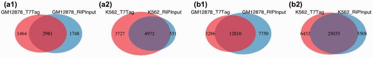
Overlap of peaks from RIPSeeker for the same protein between different controls. The primary goal of this analysis is to examine the robustness of RIPSeeker on data generated for the same protein using two different controls. Specifically, protein–RNA interaction sites for protein (a1, a2) PABPC1 and (b1, b2) ELAVL1 were predicted as peaks in cell lines GM12878 and K562 by comparing the RIP signal with the background generated from either non-specific antibody against T7-tag (T7Tag) (red) or RIP total input RNA (RIPInput) (blue) as two different types of negative control library for the protein–RNA-specific interactions. A high proportion of overlap is expected between different controls within the cell line for the same protein. For an alternative representation of a full four-way comparison, please refer to Supplementary Figure S10.
Peak lengths
The peak length distributions are presented in boxplots in Supplementary Figure S6a–l, and as reference, we also included the lengths of known transcripts from mouse and human (Supplementary Figure S6m and n). For RIP-SEQ data (Supplementary Figure S6a–j), we consistently observe that RIPSeeker, HPeak and QuEST predict peaks having lengths within the range from 100 to 10,000 nt, demonstrating their dynamic ranges in predicting relatively short and long transcribed regions. Although the underlying algorithms considerably differ among these programs, each of them has the ability to infer read-enriched regions based on adjacent signals using either transition probability from the HMM (HPeak and RIPSeeker) or the Gaussian kernel smoothing technique (QuEST). In contrast, the ranges of peak lengths predicted by RIPSeeker on the PAR-CLIP data (Supplementary Figure S6k and l) are much smaller, ranging from 50 to 800 nt. Indeed, the PAR-CLIP aims to identify at single-nucleotide resolution, the direct protein–RNA interaction sites through  conversion induced by the cross-linking around the binding sites. To this regard, the software MACS and PARalyzer seem to achieve a more focused range than RIPSeeker and HPeak. Nonetheless, it is still remarkable to observe that the HMM-based models are able to adapt to the variable signal ranges intrinsic to the experimental protocols.
Overlap between predictions
To examine the overall agreements between the comparison algorithms on the same datasets, we computed the pairwise overlaps between the (pooled and merged) peak lists from any two methods. The two peaks or transcripts are considered overlapped if they share at least one nucleotide. These comparisons are presented in Supplementary Figure S7 as the percentage of peaks from one method (row) that overlap with any peak from another method (column) (10). Overall, we observe reasonably good pairwise overlap percentages (generally >50%) between RIPSeeker and other methods and between other pairs as well. In addition, substantial overlaps are observed beyond pairwise comparison, as illustrated in the three-way and four-way comparison diagrams for select RIP-seq and PAR-CLIP datasets (Supplementary Figures S8 and S9).
ROC evaluation on sensitivity and specificity
The substantial pairwise and multi-way overlaps observed above provided the ground for a more rigorous comparison among the candidate methods using ROC plot (Section Receiver operating curve). Figure 6 presents the ROC plots of each method as unbiased quantitative benchmarks on their performances on each of the 12 tests derived from the 12 RIP versus control comparisons. The intuition behind such comparison is that peaks consistently agreed on among the majority of the methods convey higher confidence of being the bona fide protein-RNA binding sites and deemed to be the ‘gold-standard’ despite the lack of experimental validation. By continuously relaxing the scoring cutoff, each method will have a strictly increasing number of ‘true positive’ peaks over all of the ‘positive’ peaks it has in common with the ‘gold-standard’ set (i.e. True-positive rate TPR on the y-axis), and, meanwhile, a strictly increasing number of ‘false positive’ peaks over all of the negative peaks it has that are not in the ‘gold-standard’ set (i.e. False positive rate FPR on the x-axis). Thus, each method with at least one TP and one TN will eventually reach 100% TPR and FPR when the cutoff is relaxed to the minimum (i.e. all of the peaks from that method are included).
Figure 6.


Receiver operating curve (ROC). To examine the sensitivity and specificity of each method, we define the ‘gold-standard’ as a set of peaks consistently ‘agreed’ on by the majority of the tested programs on the same dataset. Different peaks from two methods ‘agree’ if they overlap each other or are within 1000 nt distance. For each of the 12 RIP versus control comparisons (a)–(l), the ROC corresponding to each method is plotted by iteratively evaluating true-positive rate (y-axis) and false-positive rate (x-axis) based on the increasing score-specific cutoff for each program. Except for (b) RIP-seq CCNT1, where RIPScore was used, −log10(P-value) was used to construct the ROC for RIPSeeker. ROC for Cuffdiff is absent in some plots due to insufficient data to have at least one TP and one FP. Please refer to Receiver operating curve for more details.
However, a sensible method will have TPR increasing much faster than the FPR with relaxing cutoff. The resulting ROC will cross the second quadrant of the plot (i.e. the top left corner) and have area under the curve (AUC) much greater than 50%. This is the case for RIPSeeker in all of the 12 ROCs and other methods such as QuEST and HPeak in most of the tests. Remarkably, RIPSeeker dominates the majority of the tests (9 of 12) in terms of AUC, with large leading margin ahead of the second best method in most of the cases. Together, RIPSeeker has consistently demonstrated its superiority over other methods in terms of sensitivity and specificity in identifying confidence peaks.
Genomic composition of peaks
To further compare the plausibility of the peaks identified by each method, we examined the proportion of peaks overlapping with basic genomic elements. Similar to that described in (35), each peak is assigned with exactly one genomic feature according to the following order of preference: 5′-UTR, coding sequence (CDS), 3′-UTR, intronic and intergenic regions based on Ensembl 65 and 69 for mouse and human, respectively.
Except for PRC2 and CCNT1, we found biologically meaningful and statistically significant binding preference toward one or two genomic elements for the proteins examined based on hypergeometric test (Supplementary Figure S11). Such preference is consistently agreed on among the methods, which performed competitively in the ROC test (Figure 6). Specifically, ELAVL1 exhibits significant bias toward intronic and 3′-UTR regions (P < 2.2e-308 and P < 8.0e-55, respectively, for the RIPSeeker peaks) regardless of the distinct cell lines and negative controls (Supplementary Figure S11c–f). Indeed, ELAVL1 (or HuR) has been implicated in regulation of multiple alternative pre-mRNA splicing and also functions by interacting with AU-rich sequence elements (ARE) frequently found within 3′-UTRs (37). For PABPC1, on the other hand, we observe consistently significant enrichment for 3′-UTR among the peaks from the competitive methods (Supplementary Figure S11g–j). Indeed, PABPC1 predominantly acts at the 3′-UTR for poly(A) shortening (38). Binding of PABPC1 is also responsible for ribosome recruitment and translation initiation, which may explain the seemingly (but not statistically) significant enrichment for CDS (38).
For the other two well-studied proteins PUM2 and QKI, all of the four comparison methods (MACS, HPeak, RIPSeeker and PARalyzer) have PAR-CLIP peaks significantly enriched for 3′-UTR and intronic elements, respectively, and both having P-value <2.2e-308 based on hypergeometric tests (Supplementary Figure S11k and l). Indeed, PUM2 is known to regulate the translation and stability of mRNA through binding to their 3′-UTR regions; QKI is well-characterized splicing regulator found in intronic regions (35). Together, the results suggest that the peaks identified by the methods promising in the ROC evaluation (Section ROC evaluation on sensitivity and specificity) are enriched for common biologically meaningful genomic elements according to the literature, further demonstrating the sensibility of these methods.
Motif enrichment of top peaks
To examine whether the peaks identified by each program are enriched for any meaningful motif, we applied MEME-ChIP (39) to up to 5000 top peaks from each program ranked by the program-specific scoring schemes described in Section Receiver operating curve, except that we used RIPScore to rank the peaks for RIPSeeker. The results from the motif analyses are inconclusive for most proteins, except for PUM2 and QKI, which have predicted motifs published in (35) that can be used as a reference. Remarkably, the top 5000 peaks from RIPSeeker, MACS and PARalyzer on PUM2 PAR-CLIP data are enriched for the exact PUM2 published motif in (35) as the top prediction by DREME with highly significant E-values (1e-60, 3.7e-201 and 3.3e-161 for RIPSeeker, MACS and PARalyzer, respectively) (Supplementary Figures S12–S14), whereas the top 5000 peaks from HPeak have much less significant E-values (1e-6) (Supplementary Figure S15). Notably, the PUM2 motif is not the top-ranked motif based on DREME for MACS and HPeak. Similar results are observed for QKI motif comparison, where the top 5000 peaks from each method, except HPeak, are clearly enriched for the published QKI motif, although not as strong as in the case for PUM2 (Supplementary Figure S12–S14). Notably, only PARalyzer uses the  conversion information in the alignments. The results together with the consistent genomic composition analysis on the PAR-CLIP data (Section Genomic composition of peaks) suggest that the read alignments information alone is likely to be sufficient to uncover meaningful motif patterns (if any) with a reliable peak-calling algorithm. A systematic comparison between RIP-seq and PAR-CLIP analyses on a common set of proteins is needed to confirm our findings. Nonetheless, the
  conversion enables PARalyzer to identify at the single-nucleotide resolution the protein–RNA binding sites, whereas other methods are unable to do so.
For PRC2, we found the top 1000 peaks from RIPSeeker and QuEST (the two favorable methods in the ROC test) to contain GA-rich motifs with E-values <9.5e-274 and <2.2e-162, respectively, in both biological replicates (data not shown). Interestingly, it has been shown that JARID2 (a recently identified PRC2 subunit) appears to particularly prefer GC- and GA-rich motifs in the DNA (40), but it is not clear whether the DNA-binding motif has any correlation with the RNA-binding preference and whether Ezh2 and JARID2 interact with a similar set of transcripts.
Performance on predicting known transcripts
In mESC, PRC2 is known to associate with Tsix, Xist, Kcnqo1t1 and Meg3 on + and − strands (also known as Gtl2) (4). Indeed, RIPSeeker identified all of the five transcripts with substantial base coverage by the long peaks from the PRC2 and CCNT1 datasets (Supplementary Figure S19). Furthermore, all of the RIPSeeker’s predictions fall into the correct strands of the transcripts. QuEST is also able to identify all of the positive hits with comparable coverage as RIPSeeker. In contrast, HPeak and MACS predict much shorter peaks (Supplementary Figure S19a) or miss some of the targets at the correct strand orientation (Supplementary Figure S19d). Cuffdiff failed to predict any of the five transcripts. Supplementary Figure S19a clearly illustrates that RIPSeeker’s predictions cover substantial proportion of the exonic regions belonging to Xist on the ‘−’ strand. In addition, RIPSeeker seems to suggest the existence of the longer isoform of Xist (third transcript in the ‘Refseq genes’ track), as its predictions cover the unique exonic portion of that isoform. In contrast, predictions on the same gene are much more segmented for QuEST and HPeak and punctuated for MACS.
For CCNT1, all methods, but Cuffdiff and MACS, are able to predict RN7SK on the correct strand (i.e. the + strand) (Supplementary Figure S19d). MACS is able to detect the correct loci but not the strand. It is worth emphasizing that unlike RIPSeeker, the other tested ChIP-seq algorithms do not have the ability to model strand-specific library, but rather through manipulation of input alignments (ChIP-seq programs). Additionally, RIPSeeker is the only de novo algorithm that exclusively predicts RN7SK on the + strand locus (rather than on both or on − strand), whereas QuEST and HPeak predict peaks on the − strand, likely due to the second non-strand-specific library. To our knowledge, there is no well-characterized lncRNA for the other proteins examined.
Other criteria considered
We also compared the enrichment for different biotype categories (protein coding, lincRNA, etc) (Supplementary Figure S18), averaged conservation (Supplementary Figure S16) and RNA local folding energy (Supplementary Figure S17) for the peaks identified by each method. The results are inconclusive and omitted from the main text.
DISCUSSION
In this article, we described RIPSeeker, an HMM-based R software package specifically tailored to analyze RIP-seq data with statistical rigor. As a proof-of-concept, we first tested RIPSeeker’s performance on the simulated data generated from a two-state HMM with known NB parameters and observed, on average, 85–100% accuracy (Supplementary Figure S1). To demonstrate the utility of the software package in the real-world application, we made use of three independent RIP-seq datasets and two PAR-CLIP datasets, including, in total, 12 sample comparisons corresponding to six distinct proteins (RIP-seq: PRC2, CCNT1, ELAVL1 and PABPC1; PAR-CLIP: PUM2 and QKI). As comparisons, we applied to the same datasets, six state-of-the-art algorithms, including three ChIP-seq algorithms (MACS, QuEST and HPeak), two RNA-seq methods (Cuffdiff and Rulebased) and one PAR-CLIP program (PARalyzer) (Table 1). We also tested DESeq (as the third RNA-seq strategy) on these datasets and decided not to include it in the subsequent comparisons due to the small number of significant transcripts identified by the method (detailed in Supplementary Methods Section Bioconductor package DESeq settings and results). Based on the pairwise and multi-way overlap analyses (Supplementary Figures S7–S9), RIPSeeker not only has generally good agreements (∼50% on average) with the ChIP-seq or PAR-CLIP algorithms in their predictions on the 12 sample comparisons, but also demonstrated its robustness in the consistent predictions using distinct negative controls (T7-tag and the RIP RNA input) for the same RIP treatments in the same cell line corresponding to the protein ELAVL1 or PABPC1 (Figure 5).
The observed good agreements among most of the tested methods prompted us for a more rigorous and quantitative comparison based on AUC derived from the ROC plots (Section Receiver operating curve). Due to the insufficient canonical transcripts (‘gold-standard’) known to associate with the six available proteins, we constructed for each of the 12 sample comparisons, a list of confidence peaks overlapped by peaks from the majority (at least half) of the tested methods and used such a list to benchmark each method based on their sensitivity and specificity as functions of decreasing score-specific cutoff in discriminating the confidence peaks from other peaks within their own predictions. The resulting AUCs from the ROCs were then used to evaluate and compare the performances of the comparison methods on each sample. RIPSeeker demonstrated superior performances by having the highest AUC, averaging >80% in 9 of the 12 tests (Figure 6). The results from these unbiased analyses not only consistently favor the proposed RIP-seq program but also suggest a sensible way for the users to prioritize RIPSeeker predictions based on the corresponding statistical confidence.
Some explanations are needed for some methods falling below the diagonal line of the ROC plots in some tests, which may seem worse than random. As the true-negatives TN are unknown, we used as proxy, the predictions from each method that are not in the consensus peak list (defined as the peaks consistently agreed on by a majority of the methods). Thus, the ROC is relative to each method, with the TP and TN defined as the number of predictions from that method that have overlap and no overlap with the consensus peak list, respectively. Consequently, the TP and TN are not necessarily equal. Thus, a method can have most of its peaks not in the consensus set, leading to TN much greater than TP. Moreover, if the scores from that method do not properly favor the minority of the TP, then we will observe a ROC lying at the lower triangle portion of the plot leading to <50% AUC, which can be seen with the Rulebased method and several other methods in some panels (e.g. Figure 6b–d). Conceptually, the peak callers here can be considered as ‘unsupervised classifiers’ that call peaks directly from the genome. To some extent, a completely insensible method would be equivalent to randomly sampling genomic regions from the genome. Thus, the ‘random peaks’ will unlikely to have any overlap with the peaks from other sensible methods. As a result, ROC corresponding to that method will have a flat curve along the x-axis (FPR), resulting in a zero AUC. Thus, given the large search space of a mammalian genome, a method having an AUC ∼0.5 in the current comparison is actually much better than random. If the test itself were insensible, especially when the comparison methods generally disagree, then all of the methods will have AUC ∼50% or less, which is not the case because we observe good pairwise and multi-way overlaps among the comparison methods in all of the 12 tests (Supplementary Figures S7–S9), and there are more than one method in each panel having AUC much higher than 50% (Figure 6).
Furthermore, we demonstrated at the genome scale that the peaks from RIPSeeker and other comparison methods such as QuEST and HPeak that performed competitively in the ROC evaluations are biologically meaningful. In particular, the peaks for four of the six proteins, namely, ELAVL1, PABPC1, PUM2 and QKI, are significantly enriched for genomic elements, implicating their functions suggested in the literature (Supplementary Figure S11). Moreover, the top 5000 peaks from RIPSeeker for PUM2 and QKI are the most significantly enriched for the previous published motifs. Finally, RIPSeeker demonstrates its sensitivity by identifying the canonical PRC2 and CCNT1 interacting ncRNAs with high statistical confidence and peak length close to the natural length of the lncRNAs (Supplementary Figure S19).
In terms of usability, the front-end main function ripSeek is sufficient for most applications. The function takes as the only required argument the path to alignment files (BAM/BED/SAM) and outputs predicted RIP regions. Optionally, user may indicate through cNAME which among the input file(s) is (are) control to enable eFDR calculation. If the arguments biomaRt_dataset and/or goAnno are set, ripSeek will return the annotated RIP predictions and the enriched GO terms, respectively. RIPSeeker also supports paired-end read alignments. However, there are currently no paired-end RIP-seq data available. For the interest of space, many other features such as paired-end support (using RNA-seq data), visualization of read coverage (Supplementary Figures S3 and S4), GO enrichments (Supplementary Tables S2 and S3) and programmatic access to the UCSC genome browser for visualization (Supplementary Figure S20) are not demonstrated in the main text. For more details, please refer to the R documentation and vignette that come with the package. Moreover, the mixture NB and HMM functions in RIPSeeker package are implemented as general purpose function, which can be used to model any sequential count data with arbitrary number of hidden states. In fact, most functions provided in RIPSeeker can be used as standalone functions, allowing flexible customization to suit user’s own workflow. For instance, user can choose to run HMM functions followed by disambiguating multihits to just save the alignment output as GappedAlignments object for other analyses within R. As another example, user could estimate the known transcript or gene expression in RPKM or FPKM (fragments per kilobase of million mapped reads for paired-end reads) from the RNA-seq data using computeRPKM function. Together, RIPSeeker serves as a bioinformatics suite for various computations.
Because the RNA–protein interaction may arise from associations generated after cell lysis, further experimental validation is required to confirm that the protein indeed interacts with the predicted transcript in vivo (41). Ideally, validating functional association can provide strong support to the physical interaction observed from the RIP-seq analyses. For instance, based on their RIP-seq results, Zhao et al. (4) validated the interaction between PRC2 and Meg3 (or Gtl2) through RNAi knockdown and over-expression experiments to support their hypothesis that Meg3 recruits PRC2 to repress the upstream imprint gene Dlk1.
Biological replicates are an important addition to the RIP-seq analysis to further filter out false-positives. Currently, we only provide a helper function to combine peaks identified separately from the biological replicates. As future works, RIPSeeker will incorporate biological replicates into the framework in fitting the HMM model and in hypothesis testing taking into the sample variance. Additionally, the peaks obtained by RIPSeeker may be further trimmed up to where the alignments occur and end within that region to refine the peak resolution, which facilitates accurate primer design for experimental validation. Another useful future addition will be to add an input option for RNA-seq alignments assumed to come from the same sample desirably under similar conditions as the RIP-seq experiment. In that case, RIPSeeker will weigh the peaks based on the model trained on RNA-seq data assuming a positive correlation between the RIP-seq and RNA-seq signals. Finally, the parallel computing option speeds up the computation by a factor proportional to the total number of CPU cores but may impose larger memory overhead than the singe-threading approach. Performance optimization is needed to minimize memory trace.
In perspective, RIP-seq analysis provides information for transcripts that physically interact with a regulatory protein. As the ENCODE data recently become available (1,42), it is possible to correlate the RNA mediators from RIP-seq results with the known gene targets implicated in the ChIP-seq data based on their co-expressions measured by RNA-seq across experimental conditions. With analytical frameworks currently under active development for sequencing data, an integrative approach as such is at the horizon to elucidate the global RNA regulatory network.
SUPPLEMENTARY DATA
Supplementary Data are available at NAR Online: Supplementary Tables 1–3, Supplementary Figures 1–21, Supplementary Methods and Supplementary References [43–48].
FUNDING
Ontario Research Fund - Global Leader (Round 2), and Natural Sciences and Engineering Research Council (NSERC) [327612 to Z.Z.]. Y.L. is co-funded by NSERC Canada Graduate Scholarship and Ontario Graduate Scholarship. Funding for open access charge: Ontario Research Fund - Global Leader (Round 2), and NSERC.
Conflict of interest statement. None declared.
Supplementary Material
ACKNOWLEDGEMENTS
The authors thank Xiaohua Shen and Jonathan Olsen for their valuable suggestions. They also thank the Bioconductor community for supporting the bioinformatics developments. Finally, they thank the anonymous reviewers for their extremely valuable suggestions.
REFERENCES
- 1.ENCODE Project Consortium. Identification and analysis of functional elements in 1 by the ENCODE pilot project. Nature. 2007;447:799–816. doi: 10.1038/nature05874. [DOI] [PMC free article] [PubMed] [Google Scholar]
- 2.Ulf OA, Shiekhattar R. Long non-coding RNAs and enhancers. Curr. Opin. Genet. Dev. 2011;21:194–198. doi: 10.1016/j.gde.2011.01.020. [DOI] [PMC free article] [PubMed] [Google Scholar]
- 3.Khalil A, Guttman M, Huarte M, Garber M, Raj A, Rivea Morales D, Thomas K, Presser A, Bernstein B, van Oudenaarden A. Many human large intergenic noncoding RNAs associate with chromatin-modifying complexes and affect gene expression. Proc. Natl Acad. Sci. USA. 2009;106:11667. doi: 10.1073/pnas.0904715106. [DOI] [PMC free article] [PubMed] [Google Scholar]
- 4.Zhao J, Ohsumi TK, Kung JT, Ogawa Y, Grau DJ, Sarma K, Song JJ, Kingston RE, Borowsky M, Lee JT. Genome-wide identification of polycomb-Associated RNAs by RIP-seq. Mol. Cell. 2010;40:939–953. doi: 10.1016/j.molcel.2010.12.011. [DOI] [PMC free article] [PubMed] [Google Scholar]
- 5.Guttman M, Donaghey J, Carey BW, Garber M, Grenier JK, Munson G, Young G, Lucas AB, Ach R, Bruhn L, et al. lincRNAs act in the circuitry controlling pluripotency and differentiation. Nature. 2011;477:295–300. doi: 10.1038/nature10398. [DOI] [PMC free article] [PubMed] [Google Scholar]
- 6.Mikkelsen TS, Ku M, Jaffe DB, Issac B, Lieberman E, Giannoukos G, Alvarez P, Brockman W, Kim T-K, Koche RP, et al. Genome-wide maps of chromatin state in pluripotent and lineage-committed cells. Nature. 2007;448:553–560. doi: 10.1038/nature06008. [DOI] [PMC free article] [PubMed] [Google Scholar]
- 7.Margueron R, Reinberg D. The Polycomb complex PRC2 and its mark in life. Nature. 2011;469:343–349. doi: 10.1038/nature09784. [DOI] [PMC free article] [PubMed] [Google Scholar]
- 8.Michels AA, Nguyen VT, Fraldi A, Labas V, Edwards M, Bonnet F, Lania L, Bensaude O. MAQ1 and 7SK RNA interact with CDK9/cyclin T complexes in a transcription-dependent manner. Mol. Cell. Biol. 2003;23:4859–4869. doi: 10.1128/MCB.23.14.4859-4869.2003. [DOI] [PMC free article] [PubMed] [Google Scholar]
- 9.D’Orso I, Frankel AD. RNA-mediated displacement of an inhibitory snRNP complex activates transcription elongation. Nat. Struct. Mol. Biol. 2010;17:815–821. doi: 10.1038/nsmb.1827. [DOI] [PMC free article] [PubMed] [Google Scholar]
- 10.Wilbanks EG, Facciotti MT. Evaluation of algorithm performance in ChIP-seq peak detection. PloS One. 2010;5:e11471. doi: 10.1371/journal.pone.0011471. [DOI] [PMC free article] [PubMed] [Google Scholar]
- 11.Zhang Y, Liu T, Meyer CA, Eeckhoute J, Johnson DS, Bernstein BE, Nusbaum C, Myers RM, Brown M, Li W, et al. Model-based analysis of ChIP-Seq (MACS) Genome Biol. 2008;9:R137. doi: 10.1186/gb-2008-9-9-r137. [DOI] [PMC free article] [PubMed] [Google Scholar]
- 12.Valouev A, Johnson DS, Sundquist A, Medina C, Anton E, Batzoglou S, Myers RM, Sidow A. Genome-wide analysis of transcription factor binding sites based on ChIP-Seq data. Nat. Methods. 2008;5:829–834. doi: 10.1038/nmeth.1246. [DOI] [PMC free article] [PubMed] [Google Scholar]
- 13.Trapnell C, Pachter L, Salzberg SL. TopHat: discovering splice junctions with RNA-Seq. Bioinformatics. 2009;25:1105–1111. doi: 10.1093/bioinformatics/btp120. [DOI] [PMC free article] [PubMed] [Google Scholar]
- 14.Hafner M, Landthaler M, Burger L, Khorshid M, Hausser J, Berninger P, Rothballer A, Ascano M, Jungkamp A-C, Munschauer M, et al. Transcriptome-wide identification of RNA-binding protein and microRNA target sites by PAR-CLIP. Cell. 2010;141:129–141. doi: 10.1016/j.cell.2010.03.009. [DOI] [PMC free article] [PubMed] [Google Scholar]
- 15.Trapnell C, Williams BA, Pertea G, Mortazavi A, Kwan G, van Baren MJ, Salzberg SL, Wold BJ, Pachter L. Transcript assembly and quantification by RNA-Seq reveals unannotated transcripts and isoform switching during cell differentiation. Nat. Biotechnol. 2010;28:516–520. doi: 10.1038/nbt.1621. [DOI] [PMC free article] [PubMed] [Google Scholar]
- 16.Roberts A, Goff L, Pertea G, Kim D, Kelley DR, Pimentel H, Salzberg SL, Rinn JL, Pachter L, Trapnell C. Differential gene and transcript expression analysis of RNA-seq experiments with TopHat and Cufflinks. Nat. Protoc. 2012;7:562–578. doi: 10.1038/nprot.2012.016. [DOI] [PMC free article] [PubMed] [Google Scholar]
- 17.Anders S, Huber W. Differential expression analysis for sequence count data. Genome Biol. 2010;11:R106. doi: 10.1186/gb-2010-11-10-r106. [DOI] [PMC free article] [PubMed] [Google Scholar]
- 18.Rabiner L. A tutorial on hidden Markov models and selected applications in speech recognition. Proc. IEEE. 1989;77:257–286. [Google Scholar]
- 19.Bishop C. Pattern recognition and machine learning. In: Jordan M, Kleinberg J, Schölkopf B, editors. Information Science and Statistics. NY, USA: Springer Science+Business Media; 2006. pp. 605–631. [Google Scholar]
- 20.Qin ZS, Yu J, Shen J, Maher CA, Hu M, Kalyana-Sundaram S, Yu J, Chinnaiyan AM. HPeak: an HMM-based algorithm for defining read-enriched regions in ChIP-Seq data. BMC Bioinformatics. 2010;11:369. doi: 10.1186/1471-2105-11-369. [DOI] [PMC free article] [PubMed] [Google Scholar]
- 21.Cloonan N, Forrest ARR, Kolle G, Gardiner BBA, Faulkner GJ, Brown MK, Taylor DF, Steptoe AL, Wani S, Bethel G, et al. Stem cell transcriptome profiling via massive-scale mRNA sequencing. Nat. Methods. 2008;5:613–619. doi: 10.1038/nmeth.1223. [DOI] [PubMed] [Google Scholar]
- 22.Aboyoun P, Pages H, Lawrence M. GenomicRanges: representation and manipulation of genomic intervals. 2012 R package version 1.8.9. [Google Scholar]
- 23.Song Q, Smith AD. Identifying dispersed epigenomic domains from ChIP-Seq data. Bioinformatics. 2011;27:870–871. doi: 10.1093/bioinformatics/btr030. [DOI] [PMC free article] [PubMed] [Google Scholar]
- 24.Shimazaki H, Shinomoto S. A method for selecting the bin size of a time histogram. Neural Comput. 2007;19:1503–1527. doi: 10.1162/neco.2007.19.6.1503. [DOI] [PubMed] [Google Scholar]
- 25. Pages,H., Aboyoun,P. and Lawrence,M. (2012) IRanges: Infrastructure for manipulating intervals on sequences R package version 1.14.4.
- 26.Meng X. Maximum likelihood estimation via the ECM algorithm: a general framework. Biometrika. 1993;80:267–278. [Google Scholar]
- 27.Benjamini Y, Hochberg Y. Controlling the false discovery rate: a practical and powerful approach to multiple testing. J. R. Stat. Soc. Ser. B. 1995;57:289–300. [Google Scholar]
- 28. Lawrence,M., Gentleman,R. and Carey,V. (2009) rtracklayer: an R package for interfacing with genome browsers. Bioinformatics, 25, 1841–1842. [DOI] [PMC free article] [PubMed]
- 29.Durinck S, Moreau Y, Kasprzyk A, Davis S, De Moor B, Brazma A, Huber W. BioMart and Bioconductor: a powerful link between biological databases and microarray data analysis. Bioinformatics. 2005;21:3439–3440. doi: 10.1093/bioinformatics/bti525. [DOI] [PubMed] [Google Scholar]
- 30.Durinck S, Spellman P, Birney E. Mapping identifiers for the integration of genomic datasets with the R/Bioconductor package biomaRt. Nat. Protoc. 2009;4:1184–1191. doi: 10.1038/nprot.2009.97. [DOI] [PMC free article] [PubMed] [Google Scholar]
- 31.Zhu LJ, Gazin C, Lawson ND, Pagès H, Lin SM, Lapointe DS, Green MR. ChIPpeakAnno: a Bioconductor package to annotate ChIP-seq and ChIP-chip data. BMC Bioinformatics. 2010;11:237. doi: 10.1186/1471-2105-11-237. [DOI] [PMC free article] [PubMed] [Google Scholar]
- 32.Robinson JT, Thorvaldsdóttir H, Winckler W, Guttman M, Lander ES, Getz G, Mesirov JP. Integrative genomics viewer. Nat. Biotechnol. 2011;29:24–26. doi: 10.1038/nbt.1754. [DOI] [PMC free article] [PubMed] [Google Scholar]
- 33.Mortazavi A, Williams BA, Mccue K, Schaeffer L, Wold B. Mapping and quantifying mammalian transcriptomes by RNA-Seq. Nat. Methods. 2008;5:621–628. doi: 10.1038/nmeth.1226. [DOI] [PMC free article] [PubMed] [Google Scholar]
- 34. Carlson,M., Pages,H., Aboyoun,P., Falcon,S., Morgan,M., Sarkar,D. and Lawrence,M. (2012) GenomicFeatures: tools for making and manipulating transcript centric annotations R package version 1.8.2, 2012.
- 35.Corcoran DL, Georgiev S, Mukherjee N, Gottwein E, Skalsky RL, Keene JD, Ohler U. PARalyzer: definition of RNA binding sites from PAR-CLIP short-read sequence data. Genome Biol. 2011;12:R79. doi: 10.1186/gb-2011-12-8-r79. [DOI] [PMC free article] [PubMed] [Google Scholar]
- 36.Mak AB, Ni Z, Hewel JA, Chen GI, Zhong G, Karamboulas K, Blakely K, Smiley S, Marcon E, Roudeva D, et al. A lentiviral functional proteomics approach identifies chromatin remodeling complexes important for the induction of pluripotency. Mol. Cell. Proteomics. 2010;9:811–823. doi: 10.1074/mcp.M000002-MCP201. [DOI] [PMC free article] [PubMed] [Google Scholar]
- 37.Dai W, Zhang G, Makeyev EV. RNA-binding protein HuR autoregulates its expression by promoting alternative polyadenylation site usage. Nucleic Acids Res. 2012;40:787–800. doi: 10.1093/nar/gkr783. [DOI] [PMC free article] [PubMed] [Google Scholar]
- 38.Huntzinger E, Braun JE, Heimstädt S, Zekri L, Izaurralde E. Two PABPC1-binding sites in GW182 proteins promote miRNA-mediated gene silencing. EMBO J. 2010;29:4146–4160. doi: 10.1038/emboj.2010.274. [DOI] [PMC free article] [PubMed] [Google Scholar]
- 39.Machanick P, Bailey TL. MEME-ChIP: motif analysis of large DNA datasets. Bioinformatics. 2011;27:1696–1697. doi: 10.1093/bioinformatics/btr189. [DOI] [PMC free article] [PubMed] [Google Scholar]
- 40.Herz H-M, Shilatifard A. The JARID2-PRC2 duality. Genes Dev. 2010;24:857–861. doi: 10.1101/gad.1921610. [DOI] [PMC free article] [PubMed] [Google Scholar]
- 41.Mili S, Steitz JA. Evidence for reassociation of RNA-binding proteins after cell lysis: implications for the interpretation of immunoprecipitation analyses. RNA. November, 2004;10:1692–1694. doi: 10.1261/rna.7151404. [DOI] [PMC free article] [PubMed] [Google Scholar]
- 42.Gerstein MB, Kundaje A, Hariharan M, Landt SG, Yan K-K, Cheng C, Mu XJ, Khurana E, Rozowsky J, Alexander R, et al. Architecture of the human regulatory network derived from ENCODE data. Nature. 2013;488:91–100. doi: 10.1038/nature11245. [DOI] [PMC free article] [PubMed] [Google Scholar]
- 43.Langmead B, Trapnell C, Pop M, Salzberg SL. Ultrafast and memory-efficient alignment of short DNA sequences to the human genome. Genome Biol. 2009;10:R25. doi: 10.1186/gb-2009-10-3-r25. [DOI] [PMC free article] [PubMed] [Google Scholar]
- 44.Li H, Handsaker B, Wysoker A, Fennell T, Ruan J, Homer N, Marth G, Abecasis G, Durbin R, 1000 Genome Project Data Processing Subgroup The sequence alignment/map format and SAMtools. Bioinformatics. 2009;25:2078–2079. doi: 10.1093/bioinformatics/btp352. [DOI] [PMC free article] [PubMed] [Google Scholar]
- 45.Martin M. Cutadapt removes adapter sequences from high-throughput sequencing reads. EMBnet J. 2011;17:10–12. [Google Scholar]
- 46.Quinlan AR, Hall IM. BEDTools: a flexible suite of utilities for comparing genomic features. Bioinformatics. 2010;26:841–842. doi: 10.1093/bioinformatics/btq033. [DOI] [PMC free article] [PubMed] [Google Scholar]
- 47.Roberts A, Pimentel H, Trapnell C, Pachter L. Identification of novel transcripts in annotated genomes using RNA-Seq. Bioinformatics. 2011;27:2325–2329. doi: 10.1093/bioinformatics/btr355. [DOI] [PubMed] [Google Scholar]
- 48.Lorenz R, Bernhart SH, Höner Zu Siederdissen C, Tafer H, Flamm C, Stadler PF, Hofacker IL. ViennaRNA Package 2.0. Algorithms Mol. Biol. 2011;6:26. doi: 10.1186/1748-7188-6-26. [DOI] [PMC free article] [PubMed] [Google Scholar]
Associated Data
This section collects any data citations, data availability statements, or supplementary materials included in this article.