Critical mass hypothesis revisited: role of dynamical wave stability in spontaneous termination of cardiac fibrillation

Abstract

The tendency of atrial or ventricular fibrillation to terminate spontaneously in finite-sized tissue is known as the critical mass hypothesis. Previous studies have shown that dynamical instabilities play an important role in creating new wave breaks that maintain cardiac fibrillation, but its role in self-termination, in relation to tissue size and geometry, is not well understood. This study used computer simulations of two- and three-dimensional tissue models to investigate qualitatively how, in relation to tissue size and geometry, dynamical instability affects the spontaneous termination of cardiac fibrillation. The major findings are as follows: 1) Dynamical instability promotes wave breaks, maintaining fibrillation, but it also causes the waves to extinguish, facilitating spontaneous termination of fibrillation. The latter effect predominates as dynamical instability increases, so that fibrillation is more likely to self-terminate in a finite-sized tissue. 2) In two-dimensional tissue, the average duration of fibrillation increases exponentially as tissue area increases. In three-dimensional tissue, the average duration of fibrillation decreases initially as tissue thickness increases as a result of thickness-induced instability but then increases after a critical thickness is reached. Therefore, in addition to tissue mass and geometry, dynamical instability is an important factor influencing the maintenance of cardiac fibrillation.

Ventricular Fibrillation (VF) is usually sustained, but episodes of spontaneous termination have been observed (5, 7, 10, 29, 44) and, in the experimental setting, depend on tissue size (15, 23). Atrial fibrillation (AF) is classified into three subtypes (2): 1) paroxysmal, i.e., AF that terminates spontaneously after no more than a few days; 2) persistent, i.e., AF that does not terminate spontaneously but can be cardioverted to sinus rhythm electrically or with use of antiarrhythmic drugs; and 3) permanent, i.e., AF that cannot be converted to sinus rhythm. Spontaneous termination of AF is widely observed (21, 54). Ninety years ago, Garrey (15) observed that persistence of fibrillation depended on tissue mass and form, leading to the well-known “critical mass hypothesis.” Zipes et al. (60) showed that VF terminated when a critical amount of tissue was depolarized in dog ventricles. Recent clinical studies have also shown that termination of AF by drugs (25) and ablation (6, 26) depends on the size of the left atrium. On the basis of spiral wave reentry theory (4, 43), if fibrillation is due to or driven by a stable spiral wave (rotor), such as in the “mother rotor hypothesis” (59), only a critical size corresponding to an area slightly larger than the spiral core will be required to sustain fibrillation. In other words, as long as the tissue size is larger than the core of the stable rotor, the arrhythmia is sustained and will not self-terminate. If the arrhythmia is due to spiral wave meander or breakup caused by dynamical instabilities (43), as described in “multiple-wavelet hypothesis” (30) as “irregular wondering of numerous wavelets,” a much larger critical size is required for sustained fibrillation.

Effective therapies must prevent arrhythmia initiation or terminate the arrhythmia quickly after initiation. Therefore, understanding the mechanisms of arrhythmia termination could potentially be as important as understanding the mechanisms of initiation. Despite the widely observed spontaneous termination of arrhythmias in atria and ventricles, few studies have been carried out to address the determinants of persistent vs. self-terminating arrhythmias. The widely accepted theory based on the critical mass hypothesis and the multiple-wavelet hypothesis is that maintenance and self-termination of arrhythmias are regulated by the wavelength relative to tissue size. Other factors, such as dynamical instability, tissue heterogeneity, and tissue geometry and structure, have not been comprehensively investigated. In this study, computer simulations of two-dimensional (2-D) and three-dimensional (3-D) tissue models were used to investigate how dynamical wave stability and tissue geometry regulate self-termination of cardiac fibrillation. In 2-D tissue, phase I of the Luo and Rudy (LR1) action potential model (28) and a two-variable model developed by Bär and Eiswirth (4) for a generic excitable medium (Bär model) were simulated. In 3-D tissue, only the Bär model was simulated. The rationale for using the simple models is as follows: 1) The goal of this study is to qualitatively understand the effects of dynamical instability and tissue properties on maintenance of fibrillation, rather than to quantitatively compare simulation with real fibrillation. 2) The use of simple models allows us to carry out a large number of simulations to evaluate statistically the average duration of fibrillation in a relatively large tissue. The conclusions from these simple models provide a theoretical basis for future quantitative studies, with more realistic action potential and tissue models used as tools to illuminate experimental observations in intact atrial and ventricular tissue.

Methods

Mathematical Model

A homogeneous 2-D tissue model with the LR1 ventricular action potential model (28) was simulated by using the following differential equation with no-flux boundary conditions

$$\frac{\partial V}{\partial t}=-I_{\text{ion}}/C_{\text{m}}+D(\frac{{\partial }^{2}V}{\partial x^2}+\frac{{\partial }^{2}V}{\partial y^2})$$ (1)

where V is transmembrane potential, C_m = 1 μF/cm² is membrane capacitance, and D is diffusion constant, which was set to 0.001 cm²/ms. I_ion is the total ionic current density of the membrane from the LR1 model. In this study, we used Ḡ_Na = 16 mS/cm² and Ḡ_K = 0.423 mS/cm², and most of the simulations used Ḡ_si = 0.052 mS/cm² (where Ḡ_Na,Ḡ_K, and Ḡ_si represent mean Na⁺, K⁺, and slow inward current conductance, respectively). Other parameters are the same as in the original LR1 model (28). At this parameter setting, the baseline conduction velocity is 0.55 m/s, action potential duration (APD) is shortened to 200 ms from 360 ms in the original model, and the APD restitution curve is similar to those measured from animal experiments (17, 33). One important consequence of this modification is that spiral wave breakup leading to spatiotemporal chaos or multiple-wavelet fibrillation occurs in homogeneous 2-D tissue with an average cycle length of 103 ms (41, 43). To simulate an obstacle in the homogeneous 2-D tissue, a circular area was electrically disconnected from the other area by setting D = 0 in the circular area. This is equivalent to a circular hole in the center with no-flux boundary.

Homogeneous 2-D and 3-D tissue models with a two-variable model developed by Bär and Eiswirth (4) for generic excitable medium were simulated with the following differential equations

$$\frac{\partial u}{\partial t}=f(u,v)+{\nabla }^{2}u,\frac{\partial v}{\partial t}=g(u,v)$$ (2)

where u and v are variables ranging from 0 to 1 and f and g are functions

$$\begin{array}{c}f(u,v)=u(u-1)(u-\frac{v+b}{a})/\varepsilon ,\\ g(u,v)=\{\begin{array}{cc}-v,& u<1/3\\ u-v,& 1/3\le u\le 1\\ 1-v,& u>1\end{array}\end{array}$$ (3)

Arbitrary units were used for the parameters and variables; a and b were fixed at 0.84 and 0.07, respectively. Figure 1A shows a single-cell action potential and a spiral breakup snapshot in tissue for ∊ = 0.075. The average cycle length during breakup is 5.4.

Fig. 1.

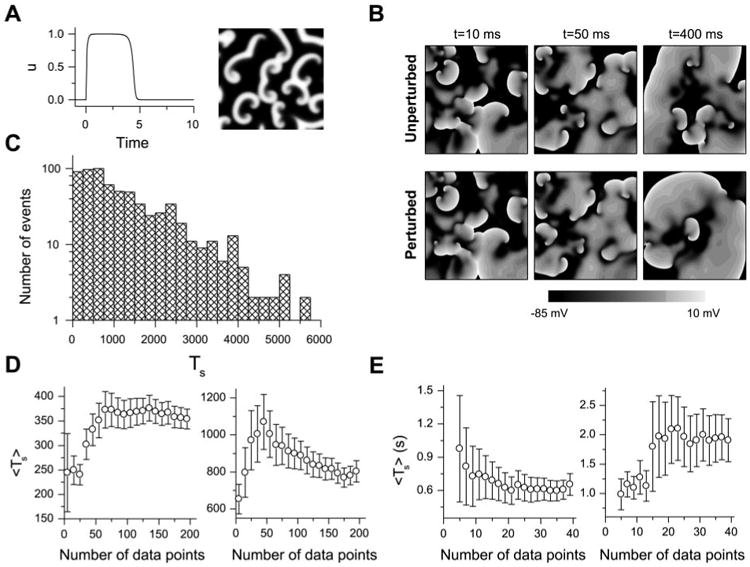
A: u vs. time for a single cell (left) and a snapshot of u during spiral wave breakup in a 42 × 42 tissue (right) for the Bär model. B: comparison of simulated fibrillation patterns in a 10 × 10-cm² tissue with the Luo and Rudy (LR1) model for an unperturbed and a randomly perturbed initial condition; at 400 ms, the patterns are very different. C: transient time (T_s) distribution in 2-dimensional (2-D) tissue with the Bär model (total 656 transients, ∊ = 0.075, tissue size = 26.25 × 26.25). D: averaged T_s (T_s) vs. number of data points used to calculate T_s for the Bär model in a 21 × 21 (left) and a 24.5 × 24.5 (right) tissue. E: T_s vs. number of data points used to calculate T_s for the LR1 model in a 7.5 × 7.5-cm² (left) and an 8.75 × 8.75-cm² (right) tissue.

Numerical Methods

A previously developed numerical method (38) was used with a time step adaptively varying from 0.02 to 0.2 ms and fixed space step Δx = Δy = 0.025 cm for the LR1 model. The explicit Euler method was used with a time step of 0.015 and a space step of 0.35 in the simulations of the Bär model for 2-D and 3-D tissues.

APD Restitution

APD restitution is defined as the present APD as a function of the previous diastolic interval (DI). APD is defined as the duration of V greater than −72 mV and DI as the duration of V less than −72 mV. APD restitution was measured in a 2-cm one-dimensional cable with a regular S1 pacing train of 500 ms followed by a premature S2 at one end of the cable.

Fibrillation Duration

Initial conditions of multiple spiral waves were used and randomly perturbed to give rise to nonsustained fibrillation with different durations. For the LR1 model, V was perturbed as

$$V(x,y,t=0)=V_0(x,y)+0.8[V_0(x,y)+80][\xi (x,y)-0.5]$$ (4)

where V₀(x,y) is the transmembrane potential of the prestored spiral waves and ξ(x,y) is a uniformly distributed random number in [0,1] for the location (x,y) and only applied at time 0. Similarly, for the Bär model, both variables were perturbed as

$$\begin{array}{c}u(x,y,z,t=0)=u_0(x,y)+0.25[\xi (x,y,z)-0.2]\\ v(x,y,z,t=0)=v_0(x,y)+0.25[\xi (x,y,z)-0.2]\end{array}$$ (5)

Because of the chaotic nature of spiral wave breakup, this perturbation results in very different fibrillation patterns (41), which then affect T_s. Figure 1B shows how such random perturbations cause very different fibrillation patterns in a homogeneous 2-D tissue with the LR1 model. Figure 1C shows a distribution of fibrillation transient time (or T_s) in 2-D tissue with the Bär model, showing an exponential decaying distribution. This indicates that these transients are statistically independent. T_s was defined as the interval from the start of fibrillation until the tissue becomes quiescent. For the Bär model, we used 200 T_s in 2-D tissue and 100 T_s in 3-D tissue to calculate the average T_s (T_s). For the simulations of 2-D tissue with the LR1 model, we used 20–40 T_s to calculate T_s. To justify these choices, Fig. 1, D and E, shows T_s and the error bars vs. the number of T_s used for both models. For the Bär model, the fluctuations in T_s and error bars begin to be small when the number of T_s is >80. For the LR1 model, the changes begin to be small when the number of T_s is >20.

Tip of Spiral Wave

Tips of spiral waves were defined as the points at which successive isovoltage lines intersect at −30 mV measured at 1-ms intervals (40).

Lyapunov Exponent

The Lyapunov exponent (λ) is a quantitative measurement of dynamical instability that is widely used in nonlinear dynamics (50). It measures how fast a small perturbation to an equilibrium state or a chaotic attractor increases (if it is positive) or decreases (if it is negative). λ is mathematically defined as

$$\lambda =\frac{1}{T}\underset{T\to \infty }{\ln }\frac{\Vert \delta \overrightarrow{X}\left(T\right)\Vert }{\Vert \delta \overrightarrow{X}\left(0\right)\Vert }$$ (6)

where δX⃗(0) is the perturbation vector to the stationary state and SX⃗(T) is the resulting vector at time T. For the Bär model in 2-D tissue, the partial differential equations for the perturbation are

$$\begin{array}{c}\frac{\partial \delta u}{\partial t}=\frac{\partial f(u,v)}{\partial u}\delta u+\frac{\partial f(u,v)}{\partial v}\partial v+{\nabla }^2\delta u,\\ \frac{\partial \delta v}{\partial t}=\frac{\partial g(u,v)}{\partial u}\delta u+\frac{\partial g(u,v)}{\partial v}\delta v\end{array}$$ (7)

which are obtained by inserting [u(x,y,t) and δu(x,y,t)] and [v(x,y,t) and δv(x,y,t)] into Eq. 2, with [u(x,y,t),v(x,y,t)] being the stationary (periodic or chaotic) solution of Eq. 2. By numerically solving Eqs. 2 and 7 jointly for a sufficiently long time period T, one obtains the vector δX⃗(T) = [δu(x,y,T,δv(x,y,T)] because of the initial perturbation vector δX⃗(0) = [δu(x,y,0), δv(x,y,0)] and then obtain λ using Eq. 6. In other words, u(x,y,t) and v(x,y,t) are numerically obtained from Eq. 2. By inserting u(x,y,t) and v(x,y,t) into Eq. 7, one then obtains δu(x,y,t) and δv(x,y,t) numerically from Eq. 7. A 42 × 42 tissue (in which spiral breakup persists much longer than T, which was used for calculation of λ) was used to calculate λ.

Results

Effects of Dynamical Instability on Spiral Wave Termination in Homogeneous Tissue

In simulated homogeneous cardiac tissue, dynamical instabilities can cause a spiral wave to break up into multiple irregularly meandering spiral waves (4, 43) resembling the “multiple-wavelet” fibrillation of Moe et al. (31). In the spiral wave breakup regimen, new waves are constantly created by dynamical instabilities simultaneously with self-termination of existing waves. If the rate of wave extinction exceeds the rate of new wave creation, the fibrillation-like state will persist for a limited period of time before the tissue becomes quiescent (Fig. 2). There are three ways by which a wave self-terminates (Fig. 2; see also supplemental online video at http://ajpheart.physiology.org/cgi/content/full/00668.2005/DC1): 1) two waves can annihilate each other if their tips collide, 2) a wave can run into a region of refractoriness from a previous wave, or 3) a wave can move off a tissue boundary. These processes are determined by wave stability and are very sensitive to initial conditions and perturbations due to dynamical chaos (41). Because of the chaotic nature of the wave breaks, T_s varies substantially for different initial conditions (Fig. 1, B and C). In cardiac tissue, previous studies (11, 22, 43, 57) showed that steepness of the APD restitution curve is an important determinant of the stability of spiral waves, such that a steep APD restitution slope generally promotes spiral wave breakup. Figure 3 shows how steepness of the APD restitution curve affects T_s. For the steeper APD restitution curve, T_s is shorter and wave number is lower, although the baseline APDs are similar for the two cases.

Fig. 2.

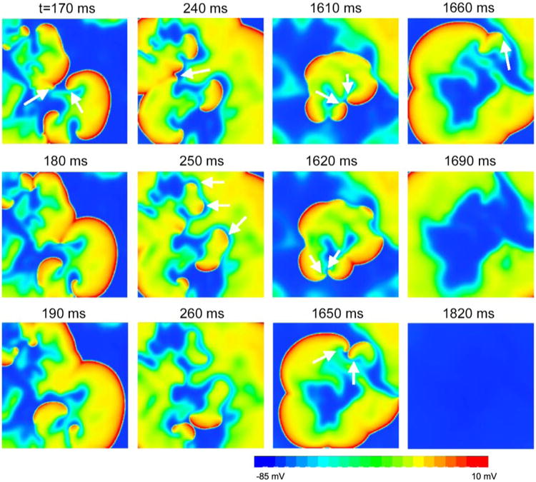
Snapshots showing self-termination of “multiple-wavelet” fibrillation from a simulation in a 10 × 10-cm² homogeneous tissue using the LR1 model. Column 1 (170–190 ms): 2 spiral waves (arrows) at 170 ms collided at 180 ms and disappeared at 190 ms. Column 2 (240–260 ms): spiral waves (arrows) at 240 and 250 ms ran into refractory tails of their previous waves and disappeared at 260 ms. Column 3 (1,610–1,650 ms): spiral pairs (arrows) collided and disappeared. Column 4 (1,660–1,820 ms): the only surviving spiral wave (arrow) moved off the tissue border, and the tissue became quiescent.

Fig. 3.

Effects of increasing dynamical instability on spiral wave breakup transient time in multiple-wavelet fibrillation in 10 × 10-cm² homogeneous tissue using the LR1 model. A: 2 action potential duration (APD) restitution curves and their slopes (inset). DI, diastolic interval. Black curve: Ḡ_si = 0.052 mS/cm²; gray curve: Ḡ_si = 0.06 mS/cm², τ_d → 0.75τ_d, τ_f → 0.75τ_f (where Ḡ_si is slow inward conductance and τ_d and τ_f represent activation and inactivation time constants, respectively). B: probability that T_s is longer than time T for APD restitution curves in A. C: T_s for the 2 cases in A. D: number of spiral wave tips vs. time for the 2 cases in A.

Because of the computational intensity of the LR1 model, its dynamics cannot be analyzed quantitatively; therefore, we simulated the simpler Bär model in 2-D tissue to probe the relation between dynamical instability and the spiral breakup transient T_s in excitable media more generally. We calculated λ for different ∊ in the breakup regime, which increases as ∊ increases (Fig. 4A). We also calculated T_s vs. ∊ for 24.5- and 26.25-cm² tissue, which decreases as ∊ increases (Fig. 4B). The plot of T_s vs. the reciprocal of λ (Fig. 4C) shows a linear relation for both tissue sizes, i.e., T_s α 1/λ. This finding indicates that as the degree of instability increases (i.e., as λ increases), T_s decreases and self-termination becomes more likely. For the LR1 model, we previously showed that as the APD restitution curve becomes steeper, λ becomes larger (43), consistent with the results in Figs. 3 and 4. Because changing a parameter of the system may also change the wavelength and spiral core size, the relation shown in Fig. 4C should not hold for the whole parameter range, rather for small ranges in which changes in dynamical instability are dominant. Indeed, the relation in Fig. 4C holds for the range shown but not for larger ranges of ∊.

Fig. 4.

Relation between dynamical instability and spiral wave breakup transient time in homogeneous tissue using the Bär model. A: Lyapunov exponent (λ) vs. ∊. B: T_s vs. ∊ for 24.5 × 24.5 (□) and 26.25 × 26.25 (■) tissues. C: T_s vs. 1/λ for 24.5 × 24.5 (□) and 26.25 × 26.25 (■) tissues.

Effects of Tissue Size and Geometry on Spiral Wave Termination in Electrically Homogeneous Tissue

Although the critical mass hypothesis was articulated 90 years ago (15), the theoretical relation between T_s and tissue size and geometry has not been comprehensively analyzed. Here we use computer simulation to study the effects of tissue size, shape, obstacles, and thickness on T_s in electrically homogeneous “fibrillating” tissue with multiple spiral waves.

Size and shape

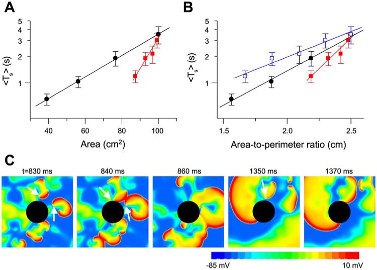
Figure 5A shows T_s vs. tissue area for square and rectangular tissues using the Bär model. For both tissue geometries, T_s increased exponentially as tissue area increased, except for small tissues, in which boundary effects increased the stability of reentry and prolonged T_s, especially for the Bär model. However, for the same total area, T_s was shorter in rectangular than in square tissues. If T_s was plotted as a function of the area-to-perimeter ratio (Fig. 5B), then the data points from the two tissue geometries fell on almost the same exponential curve. Similar results were obtained by using the LR1 model (Fig. 5, C and D). The two key findings are as follows: 1) T_s grows exponentially with tissue size, and 2) the area-to-perimeter ratio determines T_s in 2-D tissue.

Fig. 5.

Effects of tissue size and geometry on T_s in homogeneous tissue. A and B: T_s vs. tissue area and area-to-perimeter ratio, respectively, for the Bär model. ■, Square tissue; □, rectangular tissue with one side fixed at 21 arbitrary units (AU). C and D: T_s vs. tissue area and area-to-perimeter ratio, respectively, for the LR1 model with the black APD restitution curve in Fig. 3A. Fixed side for rectangular tissue is 6.25 cm. [Theoretically, the function y = a + exp(αx²) should not also be the function y = b + exp(βx), but for a small range of x, a data set may well fit both functions, which may be the case here.]

Obstacle

Anatomic obstacles in the heart include the vena cavae and pulmonary veins in the atria and the atrioventricular valves in atria and ventricles. To simulate the effects of these round obstacles on spiral breakup transients, we used a 10 × 10-cm² tissue with a circular hole in the center and the LR1 model. In the presence of a hole, T_s was much shorter than in square tissue of the same area (Fig. 6A). When T_s was plotted vs. the ratio of area to perimeter of the outer border, T_s was still shorter than in a square tissue with the same ratio (Fig. 6B). However, when T_s was plotted against the ratio of area to total perimeter of all borders (outer perimeter + perimeter of the hole), T_s was longer than in a square tissue with the same ratio (Fig. 6B). Figure 6C shows how the obstacle causes spiral waves to disappear. The role of the obstacle is twofold: 1) it provides a boundary with which spiral waves collide and self-terminate, which helps shorten the transient, and 2) a spiral wave can become anchored by the hole, converting unstable functional reentry to more stable anatomic reentry (55), which tends to prolong T_s. This latter effect may explain why T_s was longer in the tissue with the hole, despite the same area-to-total perimeter ratio as in the tissue without the hole.

Fig. 6.

Effects of obstacles on T_s. A: T_s vs. tissue area. ●, Replot of T_s in homogeneous square tissue of different sizes; red squares 10 × 10-cm² tissue with a circular hole in the center (radius = 0.5, 1.0, 1.5, or 2.0 cm). B: T_s vs. area-to-outer perimeter ratio [i.e., T_s vs. (100 cm² − πr²)/40 cm, red filled squares] and T_s vs. area-to-total perimeter ratio [i.e., T_s vs. (100 cm² − πr²)/(40 cm + 2πr²), blue open squares] for T_s in A. ●, Replot of T_s in homogeneous square tissue vs. area-to-perimeter ratio. C: snapshots illustrating disappearance of spiral waves due to the obstacle.

In the presence of a hole, the spiral wave breakup transient can terminate into quiescence or into stable reentry around the hole, similar to spontaneous conversion of AF to atrial flutter observed in animals and humans (35, 47). If the radius of the hole was small (0.5 or 1.0 cm), the tissue became quiescent after fibrillation terminated in all 30 simulations for each radius. For larger (1.5 and 2.0 cm) radii, a single stable reentry wave circulating around the obstacle remained after fibrillation terminated in 5 of the 30 simulations for each radius. In a previous study (55), we showed that unstable reentry could be stabilized when an obstacle was larger than a critical size, which depended on the degree of dynamic instability and wavelength of the reentrant wave. Conversion to stable reentry occurred when all other waves disappeared from the tissue and the remaining wave drifted to and was pinned by the obstacle. Quiescence occurred if the last wave drifted to the outer boundary instead of the obstacle. In our simulation, the conversion rate was ∼20%, which is close to the ratio of the obstacle perimeter to the outer perimeter.

Thickness

To study the effects of tissue thickness, we used the Bär model in homogeneous 3-D tissue, because the LR1 model in 3-D tissue was too computationally demanding. Figure 7 shows that, in a homogeneous 3-D tissue, T_s first increased, then decreased to a minimum, and finally increased again as tissue thickness increased. The initial decrease in T_s as tissue thickness increased may seem counterintuitive with respect to the critical mass hypothesis that greater tissue mass should sustain fibrillation longer. However, according to our previous studies in homogeneous tissue (39, 42), new instability occurs when tissue thickness exceeds a critical value. If the thickness is less than the critical value, then reentrant waves synchronize in the direction of the z-axis, forming straight scroll filaments. In this case, the 3-D tissue is equivalent to 2-D tissue, and one would expect T_s to be similar to that in 2-D tissue. However, because time is required for the spiral waves to become synchronized in the z-axis, T_s increases as tissue thickness initially increases. When the tissue thickness is greater than the critical thickness, reentrant waves desynchronize in the z-axis, forming helical scroll filaments and transmural reentry. In this case, the tissue is no longer equivalent to 2-D tissue. The new instability tends to shorten T_s, explaining the T_s decreasing phase in Fig. 7. In our previous study (42), we showed that the critical thickness was 7.3, which agrees with the thickness at which T_s begins to decrease in Fig. 7. Finally, as tissue thickness increases further, size wins over instability, causing T_s to increase again.

Fig. 7.

Effects of tissue thickness (L_z) on T_s according to the Bär model with ∊ = 0.075. x- and y-dimensions were fixed as follows: L_x = L_y = 21 AU.

Discussion

In this study, we used computer simulation of 2-D and 3-D tissue with simple action potential models to study the role of dynamic factors, in relation to tissue size and geometry, on spontaneous termination of cardiac fibrillation. The major findings from these computer simulations are as follows: 1) Dynamical instability promotes wave breaks, maintaining fibrillation, but it also causes waves to extinguish, facilitating spontaneous termination of fibrillation. The latter effect predominates as dynamical instability increases, so that fibrillation is more likely to self-terminate in a finite-sized tissue. Because of the chaotic nature of the wave breaks, T_s is sensitive to initial conditions and perturbations. T_s decreases as reentrant waves become more unstable. 2) In 2-D tissue, T_s increases exponentially as tissue area increases. In 3-D tissue, T_s decreases initially as tissue thickness increases because of thickness-induced instability but then increases after a critical thickness is reached. Therefore, in addition to tissue mass and geometry, as posited by the critical mass hypothesis, our findings indicate that dynamical instability is also an important factor in self-termination of cardiac fibrillation.

Dynamical Instability

In cardiac tissue, a steep APD restitution slope is an important cause of dynamical instability (11, 14, 16, 22, 27, 43, 45), but other causes, such as intracellular Ca²⁺ cycling, may be also important (8, 13, 37, 43, 49, 53). In the present study, we investigated the APD restitution slope as a convenient tool to modulate dynamical instability and analyze the effects on the spontaneous termination of fibrillation. We found that, in addition to its role in creating new waves that maintain multiple wavelet fibrillation, a steep APD restitution slope also enhanced the destruction of existing waves, promoting the self-termination of fibrillation in tissue with finite size and simple geometry. The simpler Bär model, in which dynamical instability is produced by a mechanism that is different from the APD restitution slope, allowed us to analyze the dynamics in more detail than was possible with the LR1 model. Most importantly, the similar findings suggest that our results represent generic effects of dynamical instability rather than specific effects related to a particular instability mechanism. On the basis of this reasoning, we believe that dynamical instability caused by other mechanisms, such as intracellular Ca²⁺ cycling, will yield similar results. However, this conjecture needs to be substantiated in more detailed models in which intracellular Ca²⁺ cycling dynamics are realistically incorporated.

Tissue Size and Geometry

The critical mass hypothesis posits that a critical tissue size is needed to support fibrillation. Garrey (15) observed that persistence of fibrillation is “directly proportional to the size of the tissue mass,” but he also noted that “form is important.” Our simulations show that T_s increases exponentially with tissue size but also depends on the tissue form. There are several ways to increase effective tissue size. 1) The actual physical tissue size can enlarge via hypertrophy and chamber dilatation. 2) Shortening of the refractory period due to remodeling shortens the wavelength, so that reentrant circuits require less tissue space. 3) Cell decoupling due to structural remodeling of gap junctions further decreases wavelength. Cell decoupling may be very effective in initiating and maintaining fibrillation (34). For example, if the gap junction conductance is reduced fourfold, a 10 × 10-cm² tissue becomes equivalent to a 20 × 20-cm² tissue, and T_s will increase from 3.5 to 20,000 s (>5,000 times) on the basis of Fig. 5C. Cell decoupling widely occurs in atrial remodeling (1) and in postinfarct remodeling and hypertrophy (3, 36), which, combined with the electrical remodeling, may substantially enhance the persistence of fibrillation.

A nonintuitive result from our simulation is that T_s did not increase simply with tissue thickness, which seems to be contrary to the critical mass hypothesis. 1) In 3-D tissue, the reentry exists as scroll waves. To terminate, the filament of the scroll wave, not just the spiral tip, must disappear. Therefore, thickness per se should not enhance the maintenance of fibrillation. 2) Thickness induces dynamical instability, which helps terminate fibrillation. In addition to tissue thickness, our simulations show that tissue geometry is also important. This could be one factor that makes AF much more likely to self-terminate than VF, because the atria have a much lower area-to-perimeter ratio due to various veins and other structures that increase the border perimeter. These results also support the rationale for the radio-frequency maze procedure and radio-frequency ablation strategies (12) in the treatment of AF. In the latter setting, our findings suggest that, in addition to ablating possible focal sources, ablation lines, which decrease the area-to-perimeter ratio, will contribute to prevention of sustained AF. However, the topology of the ventricles is very different from that of a 2-D or 3-D slab, and how it affects the maintenance of fibrillation is not clear. The conclusion that T_s increases exponentially with tissue area or area-to-perimeter ratio from simulations of 2-D and 3-D slabs may not be applicable to the ventricles. In fact, the less frequent self-termination of VF than AF may be due to larger tissue mass as well as more complex 3-D structure and topology. Computer simulations of a realistic (57) or a simplified (46) ventricle model are necessary to understand how dynamical instability interacts with the topology of the ventricles in the maintenance of fibrillation and to validate whether conclusions from simulations of 2-D and 3-D slabs are still valid.

Limitations

Primarily because of computational constraints, we used relatively simple action potential and tissue models, rather than a physiologically detailed late-generation action potential model (20, 24, 32) or an anatomically realistic tissue model (18, 46, 52, 57). These simplifications may affect the results and conclusions drawn from our simulations. 1) The LR1 model does not take into account Ca²⁺ cycling dynamics. Ca²⁺ cycling dynamics can also create dynamical instabilities (8,13, 37, 49), which may be very important for the maintenance of fibrillation, as demonstrated in the atrium (9, 19). 2) We used simple 2-D and 3-D monodomain tissue models, which are much simpler than the bidomain structures and geometries of the real atria and ventricles, which in turn may affect the spiral wave dynamics (18, 46, 48, 52, 57) and the maintenance of fibrillation. Our observation that T_s is determined by area-to-perimeter ratio was based on 2-D rectangular tissue geometries. We believe that this is an important observation, but exactly how it applies to complex geometry is not clear. However, simulations at this level of detail are computationally costly, making statistical evaluation of T_s impractical. 3) We did not take into account the electrical heterogeneities that induce spiral wave drift (51), frequency competition (58), and mother rotor fibrillation (56, 59). The first two effects may help terminate fibrillation, but the third effect facilitates maintenance of fibrillation. Because, for simulated multiple-wavelet fibrillation, addition of electrical heterogeneity into the tissue model also changes dynamical instability, we were not able to isolate the effects of electrical heterogeneity on self-termination of fibrillation in the present study. Nevertheless, our study illuminates possible mechanisms for self-termination of fibrillation, which may lead to improved drug-, electrical-, and anatomy-based strategies to terminate cardiac arrhythmias. These findings provide a strategy for further validation in simulation studies with more realistic action potential and tissue models and, ultimately, in tissue experiments.

References

- 1.Allessie M, Ausma J, Schotten U. Electrical, contractile and structural remodeling during atrial fibrillation. Cardiovasc Res. 2002;54:230–246. doi: 10.1016/s0008-6363(02)00258-4. [DOI] [PubMed] [Google Scholar]
- 2.Allessie MA, Boyden PA, Camm AJ, Kleber AG, Lab MJ, Legato MJ, Rosen MR, Schwartz PJ, Spooner PM, Van Wagoner DR, Waldo AL. Pathophysiology and prevention of atrial fibrillation. Circulation. 2001;103:769–777. doi: 10.1161/01.cir.103.5.769. [DOI] [PubMed] [Google Scholar]
- 3.Armoundas AA, Wu R, Juang G, Marban E, Tomaselli GF. Electrical and structural remodeling of the failing ventricle. Pharmacol Ther. 2001;92:213–230. doi: 10.1016/s0163-7258(01)00171-1. [DOI] [PubMed] [Google Scholar]
- 4.Bar M, Eiswirth M. Turbulence due to spiral breakup in a continuous excitable medium. Phys Rev E. 1993;48:R1635–R1637. doi: 10.1103/physreve.48.r1635. [DOI] [PubMed] [Google Scholar]
- 5.Calabro MP, Luzza F, Carerj S, Oreto G. Spontaneous termination of ventricular fibrillation. Heart. 2004;90:133. doi: 10.1136/hrt.2003.012823. [DOI] [PMC free article] [PubMed] [Google Scholar]
- 6.Chen MC, Chang JP, Guo GB, Chang HW. Atrial size reduction as a predictor of the success of radiofrequency maze procedure for chronic atrial fibrillation in patients undergoing concomitant valvular surgery. J Cardiovasc Electrophysiol. 2001;12:867–874. doi: 10.1046/j.1540-8167.2001.00867.x. [DOI] [PubMed] [Google Scholar]
- 7.Chen PS, Wu TJ, Ting CT, Karagueuzian HS, Garfinkel A, Lin SF, Weiss JN. A tale of two fibrillations. Circulation. 2003;108:2298–2303. doi: 10.1161/01.CIR.0000094404.26004.07. [DOI] [PubMed] [Google Scholar]
- 8.Choi BR, Burton F, Salama G. Cytosolic Ca2+ triggers early afterdepolarizations and torsade de pointes in rabbit hearts with type 2 long QT syndrome. J Physiol. 2002;543:615–631. doi: 10.1113/jphysiol.2002.024570. [DOI] [PMC free article] [PubMed] [Google Scholar]
- 9.Chou CC, Nihei M, Zhou S, Tan A, Kawase A, Macias ES, Fishbein MC, Lin SF, Chen PS. Intracellular calcium dynamics and anisotropic reentry in isolated canine pulmonary veins and left atrium. Circulation. 2005;111:2889–2897. doi: 10.1161/CIRCULATIONAHA.104.498758. [DOI] [PubMed] [Google Scholar]
- 10.Clayton RH, Murray A, Higham PD, Campbell RW. Self-terminating ventricular tachyarrhythmias—a diagnostic dilemma? Lancet. 1993;341:93–95. doi: 10.1016/0140-6736(93)92567-d. [DOI] [PubMed] [Google Scholar]
- 11.Courtemanche M. Complex spiral wave dynamics in a spatially distributed ionic model of cardiac electrical activity. Chaos. 1996;6:579–600. doi: 10.1063/1.166206. [DOI] [PubMed] [Google Scholar]
- 12.Cox JL, Schuessler RB, Boineau JP. The development of the maze procedure for the treatment of atrial fibrillation. Semin Thorac Cardiovasc Surg. 2000;12:2–14. doi: 10.1016/s1043-0679(00)70010-4. [DOI] [PubMed] [Google Scholar]
- 13.Eisner DA, Choi HS, Diaz ME, O'Neill SC, Trafford AW. Integrative analysis of calcium cycling in cardiac muscle. Circ Res. 2000;87:1087–1094. doi: 10.1161/01.res.87.12.1087. [DOI] [PubMed] [Google Scholar]
- 14.Garfinkel A, Kim YH, Voroshilovsky O, Qu Z, Kil JR, Lee MH, Karagueuzian HS, Weiss JN, Chen PS. Preventing ventricular fibrillation by flattening cardiac restitution. Proc Natl Acad Sci USA. 2000;97:6061–6066. doi: 10.1073/pnas.090492697. [DOI] [PMC free article] [PubMed] [Google Scholar]
- 15.Garrey WE. The nature of fibrillatory contraction of the heart: its relation to tissue mass and form. Am J Physiol. 1914;33:397–414. [Google Scholar]
- 16.Gilmour RF., Jr New approaches for identifying antiarrhythmic drug targets. Expert Opin Ther Targets. 2004;8:1–5. doi: 10.1517/14728222.8.1.1. [DOI] [PubMed] [Google Scholar]
- 17.Goldhaber JI, Xie LH, Duong T, Motter C, Khuu K, Weiss JN. Action potential duration restitution and alternans in rabbit ventricular myocytes: the key role of intracellular calcium cycling. Circ Res. 2005;96:459–466. doi: 10.1161/01.RES.0000156891.66893.83. [DOI] [PubMed] [Google Scholar]
- 18.Harrild D, Henriquez C. A computer model of normal conduction in the human atria. Circ Res. 2000;87:E25–E36. doi: 10.1161/01.res.87.7.e25. [DOI] [PubMed] [Google Scholar]
- 19.Honjo H, Boyett MR, Niwa R, Inada S, Yamamoto M, Mitsui K, Horiuchi T, Shibata N, Kamiya K, Kodama I. Pacing-induced spontaneous activity in myocardial sleeves of pulmonary veins after treatment with ryanodine. Circulation. 2003;107:1937–1943. doi: 10.1161/01.CIR.0000062645.38670.BD. [DOI] [PubMed] [Google Scholar]
- 20.Hund TJ, Rudy Y. Rate dependence and regulation of action potential and calcium transient in a canine cardiac ventricular cell model. Circulation. 2004;110:3168–3174. doi: 10.1161/01.CIR.0000147231.69595.D3. [DOI] [PMC free article] [PubMed] [Google Scholar]
- 21.Ikeda T, Uchida T, Hough D, Lee JJ, Fishbein MC, Mandel WJ, Chen PS, Karagueuzian HS. Mechanism of spontaneous termination of functional reentry in isolated canine right atrium. Evidence for the presence of an excitable but nonexcited core. Circulation. 1996;94:1962–1973. doi: 10.1161/01.cir.94.8.1962. [DOI] [PubMed] [Google Scholar]
- 22.Karma A. Electrical alternans and spiral wave breakup in cardiac tissue. Chaos. 1994;4:461–472. doi: 10.1063/1.166024. [DOI] [PubMed] [Google Scholar]
- 23.Kim YH, Garfinkel A, Ikeda T, Wu TJ, Athill CA, Weiss JN, Karagueuzian HS, Chen PS. Spatiotemporal complexity of ventricular fibrillation revealed by tissue mass reduction in isolated swine right ventricle. Further evidence for the quasiperiodic route to chaos hypothesis. J Clin Invest. 1997;100:2486–2500. doi: 10.1172/JCI119791. [DOI] [PMC free article] [PubMed] [Google Scholar]
- 24.Kneller J, Kalifa J, Zou R, Zaitsev AV, Warren M, Berenfeld O, Vigmond EJ, Leon LJ, Nattel S, Jalife J. Mechanisms of AF termination by pure sodium channel blockade in an ionically-realistic mathematical model. Circ Res. 2005;96:E35–E47. doi: 10.1161/01.RES.0000160709.49633.2b. [DOI] [PubMed] [Google Scholar]
- 25.Kochiadakis GE, Igoumenidis NE, Parthenakis FI, Chlouverakis GI, Vardas PE. Amiodarone versus propafenone for conversion of chronic atrial fibrillation: results of a randomized, controlled study. J Am Coll Cardiol. 1999;33:966–971. doi: 10.1016/s0735-1097(98)00678-0. [DOI] [PubMed] [Google Scholar]
- 26.Kosakai Y. Treatment of atrial fibrillation using the maze procedure: the Japanese experience. Semin Thorac Cardiovasc Surg. 2000;12:44–52. doi: 10.1016/s1043-0679(00)70016-5. [DOI] [PubMed] [Google Scholar]
- 27.Lee MH, Lin SF, Ohara T, Omichi C, Okuyama Y, Chudin E, Garfinkel A, Weiss JN, Karagueuzian HS, Chen PS. Effects of diacetyl monoxime and cytochalasin D on ventricular fibrillation in swine right ventricles. Am J Physiol Heart Circ Physiol. 2001;280:H2689–H2696. doi: 10.1152/ajpheart.2001.280.6.H2689. [DOI] [PubMed] [Google Scholar]
- 28.Luo CH, Rudy Y. A model of the ventricular cardiac action potential: depolarization, repolarization, and their interaction. Circ Res. 1991;68:1501–1526. doi: 10.1161/01.res.68.6.1501. [DOI] [PubMed] [Google Scholar]
- 29.Manoach M, Varon D, Neuman M, Netz H. Spontaneous termination and initiation of ventricular fibrillation as a function of heart size, age, autonomic autoregulation, and drugs: a comparative study on different species of different age. Heart Vessels Suppl. 1987;2:56–68. [PubMed] [Google Scholar]
- 30.Moe GK. On the multiple wavelet hypothesis of atrial fibrillation. Arch Int Pharmacodyn Ther. 1982;14:183–188. [Google Scholar]
- 31.Moe GK, Rheinboldt WC, Abildskov JA. A computer model of atrial fibrillation. Am Heart J. 1964;67:200–220. doi: 10.1016/0002-8703(64)90371-0. [DOI] [PubMed] [Google Scholar]
- 32.Nygren A, Fiset C, Firek L, Clark JW, Lindblad DS, Clark RB, Giles WR. Mathematical model of an adult human atrial cell: the role of K+ currents in repolarization. Circ Res. 1998;82:63–81. doi: 10.1161/01.res.82.1.63. [DOI] [PubMed] [Google Scholar]
- 33.Ohara T, Ohara K, Cao JM, Lee MH, Fishbein MC, Mandel WJ, Chen PS, Karagueuzian HS. Increased wave break during ventricular fibrillation in the epicardial border zone of hearts with healed myocardial infarction. Circulation. 2001;103:1465–1472. doi: 10.1161/01.cir.103.10.1465. [DOI] [PubMed] [Google Scholar]
- 34.Ohara T, Qu Z, Lee MH, Ohara K, Omichi C, Mandel WJ, Chen PS, Karagueuzian HS. Increased vulnerability to inducible atrial fibrillation caused by partial cellular uncoupling with heptanol. Am J Physiol Heart Circ Physiol. 2002;283:H1116–H1122. doi: 10.1152/ajpheart.00927.2001. [DOI] [PubMed] [Google Scholar]
- 35.Ortiz J, Niwano S, Abe H, Rudy Y, Johnson NJ, Waldo AL. Mapping the conversion of atrial flutter to atrial fibrillation and atrial fibrillation to atrial flutter. Insights into mechanisms. Circ Res. 1994;74:882–894. doi: 10.1161/01.res.74.5.882. [DOI] [PubMed] [Google Scholar]
- 36.Peters NS, Wit AL. Myocardial architecture and ventricular arrhyth-mogenesis. Circulation. 1998;97:1746–1754. doi: 10.1161/01.cir.97.17.1746. [DOI] [PubMed] [Google Scholar]
- 37.Pruvot E, Katra RP, Rosenbaum DS, Laurita KR. Calcium cycling as mechanism of repolarization alternans onset in the intact heart. Circulation. 2002;106:191–192. [Google Scholar]
- 38.Qu Z, Garfinkel A. An advanced numerical algorithm for solving partial differential equation in cardiac conduction. IEEE Trans Biomed Eng. 1999;49:1166–1168. doi: 10.1109/10.784149. [DOI] [PubMed] [Google Scholar]
- 39.Qu Z, Kil J, Xie F, Garfinkel A, Weiss JN. Scroll wave dynamics in a three-dimensional cardiac tissue model: roles of restitution, thickness, and fiber rotation. Biophys J. 2000;78:2761–2775. doi: 10.1016/S0006-3495(00)76821-4. [DOI] [PMC free article] [PubMed] [Google Scholar]
- 40.Qu Z, Weiss JN. Effects of Na+ and K+ channel blockade on vulnerability to and termination of fibrillation in simulated normal cardiac tissue. Am J Physiol Heart Circ Physiol. 2005;289:H1692–H1701. doi: 10.1152/ajpheart.00241.2005. [DOI] [PubMed] [Google Scholar]
- 41.Qu Z, Weiss JN, Garfinkel A. From local to global spatiotemporal chaos in a cardiac tissue model. Phys Rev E. 2000;61:727–732. doi: 10.1103/physreve.61.727. [DOI] [PubMed] [Google Scholar]
- 42.Qu Z, Xie F, Garfinkel A. Diffusion-induced 3-dimensional vortex filament instability in excitable media. Phys Rev Lett. 1999;83:2668–2671. [Google Scholar]
- 43.Qu Z, Xie F, Garfinkel A, Weiss JN. Origins of spiral wave meander and breakup in a two-dimensional cardiac tissue model. Ann Biomed Eng. 2000;28:755–771. doi: 10.1114/1.1289474. [DOI] [PubMed] [Google Scholar]
- 44.Reisin L, Blayer Y, Manoach M. Spontaneous ventricular defibrillation. Br Heart J. 1993;70:590–591. doi: 10.1136/hrt.70.6.590-b. [DOI] [PMC free article] [PubMed] [Google Scholar]
- 45.Riccio ML, Koller ML, Gilmour RF., Jr Electrical restitution and spatiotemporal organization during ventricular fibrillation. Circ Res. 1999;84:955–963. doi: 10.1161/01.res.84.8.955. [DOI] [PubMed] [Google Scholar]
- 46.Rogers JM. Wave front fragmentation due to ventricular geometry in a model of the rabbit heart. Chaos. 2002;12:779–787. doi: 10.1063/1.1483956. [DOI] [PubMed] [Google Scholar]
- 47.Roithinger FX, Karch MR, Steiner PR, Sippensgroenewegen A, Lesh MD. Relationship between atrial fibrillation and typical atrial flutter in humans: activation sequence changes during spontaneous conversion. Circulation. 1997;96:3484–3491. doi: 10.1161/01.cir.96.10.3484. [DOI] [PubMed] [Google Scholar]
- 48.Roth BJ. Frequency locking of meandering spiral waves in cardiac tissue. Phys Rev E. 1998;57:R3735–R3738. [Google Scholar]
- 49.Shiferaw Y, Watanabe MA, Garfinkel A, Weiss JN, Karma A. Model of intracellular calcium cycling in ventricular myocytes. Biophys J. 2003;85:3666–3686. doi: 10.1016/S0006-3495(03)74784-5. [DOI] [PMC free article] [PubMed] [Google Scholar]
- 50.Strogatz SH. Nonlinear Dynamics and Chaos: With Applications to Physics, Biology, Chemistry, and Engineering. Reading, MA: Addison-Wesley; 1994. [Google Scholar]
- 51.Ten Tusscher KH, Panfilov AV. Reentry in heterogeneous cardiac tissue described by the Luo-Rudy ventricular action potential model. Am J Physiol Heart Circ Physiol. 2003;284:H542–H548. doi: 10.1152/ajpheart.00608.2002. [DOI] [PubMed] [Google Scholar]
- 52.Vigmond EJ, Ruckdeschel R, Trayanova N. Reentry in a morphologically realistic atrial model. J Cardiovasc Electrophysiol. 2001;12:1046–1054. doi: 10.1046/j.1540-8167.2001.01046.x. [DOI] [PubMed] [Google Scholar]
- 53.Weiss JN, Chen PS, Qu Z, Karagueuzian HS, Garfinkel A. Ventricular fibrillation: how do we stop the waves from breaking? Circ Res. 2000;87:1103–1107. doi: 10.1161/01.res.87.12.1103. [DOI] [PubMed] [Google Scholar]
- 54.Wijffels M, Kirchhof C, Dorland R, Allessie MA. Atrial fibrillation begets atrial fibrillation—a study in awake chronically instrumented goats. Circulation. 1995;92:1954–1968. doi: 10.1161/01.cir.92.7.1954. [DOI] [PubMed] [Google Scholar]
- 55.Xie F, Qu Z, Garfinkel A. Dynamics of reentry around a circular obstacle in cardiac tissue. Phys Rev E. 1998;58:6355–6358. [Google Scholar]
- 56.Xie F, Qu Z, Garfinkel A, Weiss JN. Electrophysiological heterogeneity and stability of reentry in simulated cardiac tissue. Am J Physiol Heart Circ Physiol. 2001;280:H535–H545. doi: 10.1152/ajpheart.2001.280.2.H535. [DOI] [PubMed] [Google Scholar]
- 57.Xie F, Qu Z, Yang J, Baher A, Weiss JN, Garfinkel A. A simulation study of the effects of cardiac anatomy in ventricular fibrillation. J Clin Invest. 2004;113:686–693. doi: 10.1172/JCI17341. [DOI] [PMC free article] [PubMed] [Google Scholar]
- 58.Xie F, Qu Z, Weiss JN, Garfinkel A. Coexistence of multiple spiral waves with independent frequencies in a heterogeneous excitable medium. Phys Rev E. 2001;63:031905. doi: 10.1103/PhysRevE.63.031905. [DOI] [PubMed] [Google Scholar]
- 59.Zaitsev AV, Berenfeld O, Mironov SF, Jalife J, Pertsov AM. Distribution of excitation frequencies on the epicardial and endocardial surfaces of fibrillating ventricular wall of the sheep heart. Circ Res. 2000;86:408–417. doi: 10.1161/01.res.86.4.408. [DOI] [PubMed] [Google Scholar]
- 60.Zipes DP, Fischer J, King RM, Nicoll AD, Jolly WW. Termination of ventricular fibrillation in dogs by depolarizing a critical amount of myocardium. Am J Cardiol. 1975;36:37–44. doi: 10.1016/0002-9149(75)90865-6. [DOI] [PubMed] [Google Scholar]