Analysis of geographical disparities in temporal trends of health outcomes using space–time joinpoint regression

Abstract

Analyzing temporal trends in health outcomes can provide a more comprehensive picture of the burden of a disease like cancer and generate new insights about the impact of various interventions. In the United States such an analysis is increasingly conducted using joinpoint regression outside a spatial framework, which overlooks the existence of significant variation among U.S. counties and states with regard to the incidence of cancer. This paper presents several innovative ways to account for space in joinpoint regression: (1) prior filtering of noise in the data by binomial kriging and use of the kriging variance as measure of reliability in weighted least-square regression, (2) detection of significant boundaries between adjacent counties based on tests of parallelism of time trends and confidence intervals of annual percent change of rates, and (3) creation of spatially compact groups of counties with similar temporal trends through the application of hierarchical cluster analysis to the results of boundary analysis. The approach is illustrated using time series of proportions of prostate cancer late-stage cases diagnosed yearly in every county of Florida since 1980s. The annual percent change (APC) in late-stage diagnosis and the onset years for significant declines vary greatly across Florida. Most counties with non-significant average APC are located in the north-western part of Florida, known as the Panhandle, which is more rural than other parts of Florida. The number of significant boundaries peaked in the early 1990s when prostate-specific antigen (PSA) test became widely available, a temporal trend that suggests the existence of geographical disparities in the implementation and/or impact of the new screening procedure, in particular as it began available.

1. Introduction

Analyzing temporal trends in cancer incidence and mortality rates can provide a more comprehensive picture of the burden of the disease and generate new insights about the impact of various interventions. The analysis of temporal trends outside a spatial framework is however unsatisfactory, since it has long been recognized that there is significant variation among U.S. counties and states with regard to the incidence of cancer (Cooper et al., 2001). For example, although the introduction of new screening procedures is recognized as a main factor for the nationwide decrease in the incidence of late-stage cancer, little is known about the variability in the timing of the rise and fall of incidence among counties, racial and socioeconomic groups. Visualizing, analyzing and interpreting these geographical disparities in temporal trends should bring important information and knowledge that will benefit substantially cancer epidemiology, control and surveillance and help reducing these disparities.

Joinpoint regression (Kim et al., 2000), also known as piecewise linear regression, is increasingly used to identify the timing and extent of changes in time series of health outcomes, thanks to a public-domain software developed at the US National Cancer Institute, NCI (http://srab.cancer.gov/joinpoint/). The basic idea is to model the time series using a few continuous linear segments. These segments are joined at points called joinpoints, which represent the timing (i.e. year) for a statistically significant change in rate trend. There have been a few applications of joinpoint regression in cancer research, and it is now commonly used to characterize long-terms trends in cancer mortality in the US (Jemal et al., 2008) and foreign countries (Yang et al., 2003; Qiu et al., 2009; La Vecchia et al., 2010). Although one goal of Health People 2010 (US HHS, 2000) is to reduce health disparities according to geographic location, most analyses of temporal trends using joinpoint regression are aspatial and conducted at the National level or for a single cancer registry. One exception is the study of temporal trends in breast cancer mortality by state and race from 1975 to 2004 (DeSantis et al., 2008). Schootman et al. (2010) also explored temporal trends in geographic disparities and classified 200 counties into priority groups based on changes in breast cancer incidence rates. Yet, no map was included in these studies, despite the benefit of mapping results of trend analysis.

A popular alternative to joinpoint regression for analyzing space–time trends in health outcomes is the space–time scan statistic (Kulldorff et al., 1998) which can detect increases (decreases) of cases in the local temporal and spatial dimensions and examine whether this increase (decrease) is due to random variation or not. The basic idea is to construct cylindrical windows of increasing size in both space and time until they reach an upper size limit and test whether the observed number of cases is unlikely for a window of that size, using reference values from the entire study area. The method is flexible enough to adjust for covariates and to account for naturally occurring temporal and geographical trends when using the scan statistic for surveillance (Kleinman et al., 2005). For example, the approach was used by Sheehan and DeChello (2005) to detect areas in Massachusetts and years within the period [1988, 1997] where the proportion of prostate cancers diagnosed at late stage was significantly lower or higher than expected.

Despite some overlap the space–time scan statistic and join-point regression have very different goals. The former aims to detect space–time clusters which are aggregates of geographical units (e.g. counties) and years where an unusual increase or decrease in health outcomes occurred. On the other hands, join-point regression aims to model the rate of temporal change in health outcomes observed within each geographical unit considered separately. Joinpoint regression thus provides a finer modeling of temporal trends since unlike the scan statistic: (1) the analysis of temporal trends does not require the aggregation of geographical units, (2) annual rates of change and the associated confidence intervals can be estimated, (3) long-term projections or extrapolation can be conducted, and (4) time series in different geographical units can be compared and the parallelisms or identity of the two regression models can be tested.

Geostatistics provides a set of statistical tools for the analysis of data distributed in space and time. It allows the description of spatial patterns in the data, the incorporation of multiple sources of information in the mapping of attributes, the modeling of the spatial uncertainty and its propagation through decision-making. The approach has been tailored to the analysis of areal cancer data, such as incidence of childhood cancer recorded within electoral wards in England (Webster et al., 1994), lung cancer mortality in county of South-Eastern US (Goovaerts, 2010) or proportion of breast cancer late-stage cases diagnosed in census tracts in Michigan (Goovaerts, 2009). Applications of health geostatistics so far have been mainly spatial and include the filtering of noise in the data (disease mapping), the identification of aggregate of geographical units with significantly higher or lower values for the cancer outcomes (cluster analysis), or the detection of significant changes between cancer outcomes recorded in adjacent geographical units (boundary analysis).

There have been only a few geostatistical analyses of temporal series of cancer data. For example, Goovaerts and Jacquez (2005) applied sequential Gaussian simulation and local cluster analysis to the detection of clusters of high and low cervix cancer mortality rates recorded over all US State Economic Areas (SEA) for 9 time periods of 5 years each. The analysis was however conducted for each time period separately. Goovaerts and Xiao (2012) recently extended the geostatistical analysis to the temporal dimension using either a multivariate approach for the cluster analysis of county-level time series of prostate cancer outcomes or the repetition of the spatial boundary analysis across time. This paper proposes an alternative approach whereby the time series are first modeled using joinpoint regression, followed by the application of boundary analysis and cluster analysis to the parameters of the regression models or results of tests of hypothesis of parallelism of time trends. The approach is illustrated using times series of annual proportions of prostate cancer late-stage diagnosis available over the period 1981–2007 for each of the 67 counties in Florida.

2. Theory

2.1. Temporal joinpoint regression

Let {z(t), t = 1, …, T} be the observed proportions or rates of late-stage diagnosis recorded at T different time periods (e.g. years). Each observation z(t) is computed as the ratio d(t)/n(t), where n(t) is the total number of cases at time t, d(t) of which were diagnosed late. The log-linear version of the segmented regression model (Kim et al., 2000) takes the form:

$$\text{Log}(z(t))=\mu (t)+\epsilon (t)t=1,\dots ,T$$ (1)

where ε(t) is the residual for the t-th time, and the regression mean μ(t) is defined as a succession of (K + 1) linear segments over the time interval [a,b]:

$$\mu (t)={\beta }_0+{\beta }_{1}t+{\sum }_{k=1}^K{\delta }_k{(t-{\tau }_k)}^{+}$$ (2)

with (q)⁺ = q if q > 0 and zero otherwise. The parameter δ_k represents the difference between the slopes of the (k + 1)-th and k-th segments: δ_k = β_k+1 − β_k, while τ_k is the timing for a statistically significant change in rate trend (joinpoint) with τ₀ = a and τ_K+1 = b. For example, Fig. 1 shows how the proportion of prostate cancer cases diagnosed late in Florida changed yearly between 1981 and 2007 (T = 27). The observed time series was fitted with a regression model that includes two joinpoints: τ₁ = 1989 and τ₂ = 2000. The rate has been decreasing since the first year 1981. This decline accelerated significantly in 1989 (i.e. negative δ₁) before the rate started increasing in 2000; see parameters listed in Fig. 1.

Fig. 1.

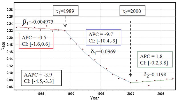
Annual proportions of prostate cancer late-stage cases (white males older than 65 years) that were diagnosed over the period 1981–2007 within Florida. The segmented regression model (solid lines) includes two joinpoints (τ) that correspond to years of statistically significant changes in rate trend: 1989 and 2000. The parameter β₁ is the slope of the first segment while the parameters δ represent the difference between the slopes of successive segments (δ_k = β_k+1 − β_k). The estimate and 95% confidence intervals of the annual percent change (APC) are computed for each segment, whereas the average annual percent change (AAPC) refers to the entire time period.

The unknowns in Eq. (2) include the number K and values τ_k of the joinpoints, as well as the regression parameters β₀, β₁ and {δ_k, k = 1, …, K}. They are estimated using a two-step procedure: (1) a grid search method (Lerman, 1980) is conducted over the set of possible joinpoints, and (2) at each step of the search the regression parameters and their standard errors are estimated by weighted least-square regression using the following criterion (Kim et al., 2000):

$$Q={\sum }_{t=1}^{T}w(t){(log(z(t))-\mu (t))}^2$$ (3)

The weights account for the fact that the variance of the residuals ε(t) may vary with time (heteroscedasticity) and they were set to n(t)/(z(t) × (1 − z(t))) for example of Fig. 1. The number K of joinpoints is estimated through an iterative procedure that tests whether models of increasing complexity (i.e. including more join-points) provide a significantly better goodness-of-fit than simpler models (Kim et al., 2009). The tests of significance use a Monte Carlo Permutation procedure described in Kim et al. (2000). To reduce the number of solutions and the computational time, a maximum number of joinpoints is typically specified (i.e. K_max = 3 here). To keep joinpoints from getting too close together or too close to either end of the time series, a minimum number of observations between joinpoints is also required and was set to 4 in the present application. This minimum number allows the computation of the standard error of the slope parameters and the associated p-values.

Trends in health outcomes over a specified time interval [τ_k, τ_k+1] are usually described by the annual percent change (APC) that, following Clegg et al. (2009), can be derived from the slope of the regression model over that time interval as:

$$\begin{array}{l}{\text{APC}}_{k+1}=100\times (exp\{{\beta }_{k+1}\}-1)\\ =100\times (exp\left\{{\beta }_1+{\sum }_{l=1}^k{\delta }_l\right\}-1)\end{array}$$ (4)

For the example of Florida, the APC is particularly large for the period [1989, 2000]: the proportion of late-stage diagnosis declined by almost 10% every year (Fig. 1). Like other regression parameters, confidence intervals can be computed for each APC and one can test whether an APC is significantly different from zero (Kim et al., 2000). Fig. 1 indicates that changes were significant only during the period 1989–2000: the 95% confidence intervals [L_APC, U_APC] computed for the segments prior to 1989 and posterior to 2000 include zero.

The trend over the entire time series [a,b] can be summarized using the average annual percent change (AAPC) which is computed as the weighted average of the APCs from the joinpoint model (Clegg et al., 2009):

$$\text{AAPC}=100\times \left(exp\left\{\frac{{\sum }_{k=1}^{K+1}{\omega }_k{\beta }_k}{{\sum }_{k=1}^{K+1}{\omega }_k}\right\}-1\right)$$ (5)

with the weight ω_k equal to the length of the APC interval [τ_k−1, τ_k]. This measure is valid even if the joinpoint model indicates that there were changes in trends during those years. Like for the APC, a (1 − α) confidence interval can be computed and if it contains zero, then there is no evidence to reject the null hypothesis that the true AAPC is zero at the significance level of α.

2.2. Space–time joinpoint regression

A spatial analysis of temporal trends can be conducted simply by applying the joinpoint regression to a set of N geographical units v_α; for example the 67 counties within the State of Florida. For any unit v_α, the regression model (1) is written as:

$$\text{Log}(z(v_{\alpha };t))=\mu (v_{\alpha };t)+\epsilon (v_{\alpha };t)t=1,\dots ,T$$ (6)

and all parameters are now county-specific: K(v_α), β₀(v_α), β₁(v_α) and {(δ_k(v_α), τ_k(v_α)), k = 1, …, K(v_α)}. As the size of the geographical units decreases, fewer cases are available for the computation of rates which become more unstable. One proposal of the present paper is to replace each rate z(v_α;t) by its noise-filtered version r̂( v_α; t) which is estimated as a linear combination of the kernel rate z(v_α;t) and the rates observed in (n−1) neighboring entities v_i at that time t:

$$\widehat{r}(v_{\alpha };t)=\sum _{i=1}^n{\lambda }_{i}z(v_i;t)$$ (7)

The weights λ_i assigned to the n rates are computed by solving a system of linear equations, known as “binomial kriging” system; see (Goovaerts, 2009) for more details. In addition, the binomial kriging variance ${\sigma }_{BK}^2(v_{\alpha };t)$ is used to compute the weighted least-square criterion (Eq. (3)):

$$w(v_{\alpha };t)=\frac{1}{{\sigma }_{BK}^2(v_{\alpha };t)}.$$

2.3. Boundary analysis

Fig. 2 shows a county map of Florida with the observed and modeled time series for a few counties, illustrating the wide range of scenarios recorded within that State. An important question in spatial epidemiology is whether temporal trends in health outcomes significantly change between neighboring units which are here defined as counties sharing a common border or vertex (1st order queen adjacencies). Detection of significant boundaries might highlight areas where causative exposures change through geographic space, the presence of local populations with distinct cancer incidences, or the impact of different cancer control methods (Jacquez, 2010).

Fig. 2.

Time series of observed proportions of prostate cancer late-stage diagnosis with the joinpoint regression model fitted for five counties in Florida. The background color of each county represents the average of its time series over the period 1981–2007.

Kim et al. (2004) proposed a permutation procedure to compare two segmented line regression functions and to test two types of hypothesis: (1) the two regression models are identical, or (2) the two mean functions are parallel allowing different intercepts. In the present paper, the later less stringent test was applied to every pair of adjacent counties (v_α, v_α′), leading to the following null and alternative hypotheses:

$$\begin{array}{l}{H}_0:(K(v_{\alpha }),\mathbf{\Theta }(v_{\alpha }))=(K(v_{{\alpha }^{\prime }}),\mathbf{\Theta }(v_{{\alpha }^{\prime }}))\text{and}\\ H_1:(K(v_{\alpha }),\mathbf{\Theta }(v_{\alpha }))\ne (K(v_{{\alpha }^{\prime }}),\mathbf{\Theta }(v_{{\alpha }^{\prime }}))\end{array}$$ (8)

where Θ( v_α) is the vector of regression parameters {β₁(v_α), (δ_k(v_α), τ_k(v_α)), k = 1, …, K(v_α)}.

To conduct a finer comparison of two segmented regression models, I also propose to compare for every time period t (i.e. year) the 95% confidence intervals of the APC for any two adjacent counties (v_α, v_α′), and count the number of times these two intervals do not overlap:

$$B_{\alpha {\alpha }^{\prime }}={\sum }_{t=1}^{T}I(\text{CI}(v_{\alpha };t);\text{CI}(v_{{\alpha }^{\prime }};t))$$ (9)

where the indicator function I(·) = 1 if the following condition on the upper bounds (U) and lower bounds (L) of the two confidence intervals CI are met: U(v_α;t) < L(v_α′;t) or L(v_α;t) > U(v_α′;t). A large number indicates that rates of changes in two adjacent counties are consistently different over time. In addition, the number of pairs of counties with non-overlapping confidence intervals for any given time t can be used to measure the extent of geographical disparities that existed at that time:

$$D(t)={\sum }_{\alpha =1}^N{\sum }_{{\alpha }^{\prime }=\alpha +1}^{N}I(CI(v_{\alpha };t);CI(v_{{\alpha }^{\prime }};t))$$ (10)

3. Case-study

3.1. The data

Number of cases of prostate cancer and associated stage at diagnosis recorded yearly from 1981 through 2007 for non-Hispanic white males within each county of Florida were downloaded from the Florida Cancer Data System website. Only cases 65 years and over were used to minimize the impact of disparities in age distribution across Florida. Proportions (rates) of late-stage diagnosis were computed over a 3-year moving window to reduce random fluctuations, yielding for each county a times series spanning 1982–2006. In this study, regional and distant cancer cases were defined as late stage.

Jemal et al. (2005) showed that non-metropolitan (non-metro) counties generally had higher death rates and incidence of late-stage disease and lower prevalence of prostate-specific antigen (PSA) screening test (53%) than metropolitan (metro) areas (58%). Following this study, results in this paper were interpreted on the basis of the US Department of Agriculture Rural–Urban Continuum Codes (USDA, 2004) described in Table 1. This nine-part county codification distinguishes metro counties by the population size of their metro area, and non-metro counties by degree of urbanization and adjacency to a metro area or areas. This information was available for 1983, 1993 and 2003. For 1983 and 1993 codes 0 and 1 were combined to make these classifications comparable to the 2003s codification. These codes were linearly interpolated over the periods 1983–1993 and 1993–2003 to explore relationships between yearly health outcomes and urbanization.

Table 1.

Definition of 2003 rural–urban continuum codes.

Code	Description
Metro counties
1	Counties in metro areas of 1 million population or more
2	Counties in metro areas of 250,000 to 1 million population
3	Counties in metro areas of fewer than 250,000 population
Non-metro counties
4	Urban population of 20,000 or more, adjacent to a metro area
5	Urban population of 20,000 or more, not adjacent to a metro area
6	Urban population of 2500–19,999, adjacent to a metro area
7	Urban population of 2500–19,999, not adjacent to a metro area
8	Completely rural or less than 2500 urban population, adjacent to a metro area
9	Completely rural or less than 2500 urban population, not adjacent to a metro area

From http://www.ers.usda.gov/data/RuralUrbanContinuumCodes/.

3.2. Space–time joinpoint regression

Yearly county-level rates of late-stage diagnosis were first noise-filtered using binomial kriging and the semivariogram computed for that year. The geostatistical filtering was conducted using the commercial software SpaceStat (BioMedware Inc., 2011). A joinpoint regression model was then fitted to each county-level noise-filtered time series using the public-domain NCI Joinpoint Regression Program, Version 3.5.0. April 2011 (NCI, 2011) which can be downloaded from http://srab.cancer.gov/joinpoint/. Results for a few counties are displayed in Fig. 2 and illustrate the wide range of behavior observed within the State of Florida. On average, the proportion of late-stage diagnosis is larger in the Big Bend region of Florida (dashed circle in Fig. 2). The geographical variability of temporal trends is summarized using two statistics that are mapped at the top of Fig. 3: the average annual percent change (AAPC, Eq. (5)) and the joinpoint corresponding to the first significant decline in proportion of late-stage diagnosis (i.e. negative APC significantly different from zero). The annual rate of decrease in prostate cancer late-stage diagnosis and the onset years vary greatly across Florida. Most counties with non-significant AAPC are located in the northwestern part of Florida, known as the Panhandle, which includes the Big Bend region (Fig. 2) and the ten counties west of it. Spatial trends are less obvious for the onset years, although the first significant decline started early in the most Western part of the Panhandle relatively to what happened in the Big bend region and on the Southwestern coast of Florida.

Fig. 3.

Maps of two parameters of the joinpoint regression models fitted to Florida county-level time series of proportions of prostate cancer late-stage diagnosis: (A) average annual percent change (APPC) over the period 1982–2006, shaded counties denote AAPC not significantly different from zero, and (B) onset year for a significant decline in proportion of late-stage diagnosis. Temporal change in the proportion of late-stage cases and rural–urban continuum code are plotted for Florida and counties grouped according to the significance of their AAPC value (C and E) and their onset year (D and F).

The maps of AAPC and onset years bear some similarities with the maps of change in rural–urban continuum codes for Florida counties over the periods 1983–1993 and 1993–2003 (Fig. 4). For most counties, the so-called Beale code decreased over time, sign of an increased urbanization. This urbanization started later (1993–2003) for the Big Bend region and south central Florida, where onset years tend to occur later as well. On the other hand, the urbanization that occurred on the southwestern coast of Florida the previous decade (Fig. 4, top) agrees fairly well with the location of the largest decline in proportion of late-stage diagnosis, as measured by the AAPC statistic (Fig. 3A).

Fig. 4.

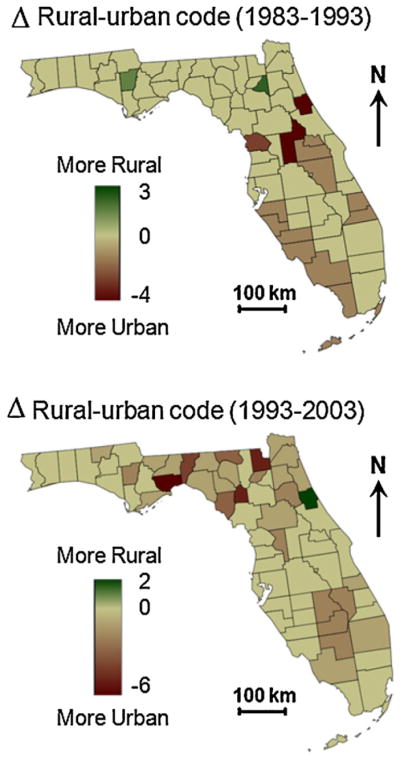
Maps of change in rural–urban continuum codes for Florida counties over the periods 1983–1993 and 1993–2003; see Table 1 for the definition of the codes.

To explore further the impact of urbanization on results, the 67 counties were grouped according to whether their AAPC is significant or not, and whether the onset year is 1990 and earlier or not. For both classification criteria, the yearly averages of proportions of late-stage diagnosis and rural–urban continuum code of counties of residence were computed for each set of counties. As expected, larger proportions of late-stage diagnosis were recorded in counties with lower rate of decline (Fig. 3C) and onset year posterior to 1990 (Fig. 3D). Yet, this trend was not observed prior to 1988. Differences between the two groups of counties are the most striking for the Beale codes. Clearly, counties with non-significant AAPC values (Fig. 3E) or non-significant decline in proportion of late-stage diagnosis prior to 1991 (Fig. 3F) tend to be on average much less urbanized (higher values of the urban–rural code) than other counties. The difference between the two groups of counties decreases with time as the overall urbanization increases.

3.3. Residual analysis

To assess the quality of the joinpoint regression models fitted to all 67 time series, the regression residuals ε( v_α;t) were computed and analyzed. The scatterplot in Fig. 5A illustrates the close fit between the noise-filtered rates and the output of the joinpoint regression model: the linear correlation coefficient is 0.976 and the residual mean of 0.0015 indicates the prediction is unbiased. The average temporal correlation among residuals computed over all 67 time series is 0.197 for Δt = 1 year and −0.094 for Δt = 2 years. Uncorrelated error models were considered here since these are the only models available in the NCI software for testing the hypothesis of coincidence or parallelisms of different trend models used in the boundary analysis.

Fig. 5.

Scatterplots of observed values versus joinpoint regression estimates (modeled values) for all 67 time series of county-level percentages of late-stage diagnosis. The scatterplots illustrate the better agreement found when conducting the join-point regression on rates that were pre-processed using binomial kriging (A) instead of the raw rates (B).

One of the novelties of the procedure described in this paper is the use of binomial kriging to filter out noise before applying joinpoint regression. To explore the impact of such filtering on the results, joinpoint regression was also performed on the time series of raw rates. Raw rates are much more variable (i.e. larger variance) than the noise-filtered rates and their use in joinpoint regression resulted in a poorer agreement between modeled and observed values (correlation is only 0.826, Fig. 5B) and a larger bias: residual mean is now −0.0124. The average residual correlation is also larger with a value of 0.279 for Δt = 1 year.

3.4. Boundary analysis

The focus of boundary analysis is on the detection of zones of rapid geographical changes (e.g. “Where do time trends in disease rates change rapidly in space?”). First, the parallelism of the mean functions fitted using joinpoint regression was tested for each pair of adjacent counties in Florida. The p-value of the test was then assigned to the common border between these two counties and used to define the thickness of the lines in Fig. 6B. Following Jacquez and Grieling (2003), an adjusted significance level α = 0.0023 was used to account for the fact that the multiple tests are not independent since near counties share similar neighbors. This level was obtained using the Bonferroni adjustment, which divides the chosen level α (here 0.01) by the average number of neighbors in each test (i.e. 4.298 here). An index of dissimilarity between each county and its neighbors was computed by averaging the p-value over all the county edges. This index is mapped in Fig. 6D. The counties that differed the most frequently from their neighbors were mainly located in Central Florida and Northeastern Florida, areas that underwent large urbanization in the eighties and nineties (Fig. 4).

Fig. 6.

Results of the space–time boundary analysis of proportion of late-stage diagnosis: (A) number of boundaries (i.e. pairs of adjacent counties) with significant differences in APC values as a function of time, (B) location of boundaries that failed the test of parallelism of the time trends for adjacent counties (thickness of black lines is inversely proportional to the p-value of the test), (C) location of boundaries between counties that display significant differences in annual percent change (APC), thickness of black lines is proportional to the number of years when the boundary was found significant. The boundary-specific results displayed in (B and C) were averaged for each county and the corresponding map represents either the average p-value of all tests of parallelism (D) or the average number of significant years per boundary (E).

Second, a finer analysis through time was undertaken by comparing for each year the confidence intervals of the APC estimate for two adjacent counties and flagging as significant all edges and years where the two intervals do not overlap. The number of significant boundaries (Eq. (10)) peaked in the early 1990s when PSA became widely available (Fig. 6A), a temporal trend that suggests the existence of geographical disparities in the implementation and/or impact of the new screening procedure, in particular as it began available. The geographical location of the most significant boundaries over the 27-year time period was derived by computing for each edge the number of years it was found significant (Eq. (9)). Boundaries that were significant at least once are depicted in black in Fig. 6C. The thickness of the black segments increases with the number of years that edge tested statistically significant (up to 15 years). An index of dissimilarity between each county and its neighbors was computed by adding up the number of significant years over all the county edges and dividing the total figure by the number of edges (Fig. 6E). Similarly to the results based on the test of parallelism of the mean functions, significant boundaries were mainly located in Central Florida and North-eastern Florida.

Three counties in Fig. 6 have an average p-value that is below the critical level α = 0.0023 and a number of significant years per edge that exceeds half the length of the time series. For two of these counties, the yearly proportions of late-stage diagnosis and rural–urban continuum code of counties of residence were compared to the averages of their neighbors (Fig. 7). The APCs of Orange County were the most often significantly different from their neighbors (14.8 years), which is reflected by very contrasted temporal trends, in particular in the eighties (Fig. 7C). Although both time series start and end with similar proportion of late-stage diagnosis, the decline started much later for Orange County and at a greater pace, maybe because of its more urbanized nature (Fig. 7E). On the other hand, Pasco County’s proportion of late-stage diagnosis was lower than its neighbors during the entire time period (Fig. 7D), a fact likely due to the strong urbanization of this county (Fig. 7F) which is part of the Tampa Bay area.

Fig. 7.

Temporal change in the proportion of late-stage diagnosis (C and D) and rural–urban continuum code (E and F) for Orange and Pasco Counties (green curve and polygon in maps A and B). These two counties displayed the most significant differences with the temporal trend of their neighbors (red curve and polygons in maps A and B) according to the space–time boundary analysis of Fig. 6. (For interpretation of the references to color in this figure legend, the reader is referred to the web version of the article.)

3.5. Cluster analysis

A natural complement to boundary analysis is provided by cluster analysis since the edge of a cluster necessarily implies a boundary (Jacquez et al., 2008). In this paper, cluster analysis aims to aggregate Florida counties based on the similarity in their temporal trends of the proportion of late-stage diagnosis. A common approach is to apply a clustering algorithm (e.g. complete linkage, kth-Nearest-Neighbor) to a matrix of dissimilarities d_αβ that quantifies the difference between any two pair of geographical units v_α and v_β. The dissimilarity was here identified with the boundary statistic B_αα′ (Eq. (9)), which was set to the length T of the time series for all non-adjacent counties in order to favor the creation of spatially compact clusters. The Ward’s minimum variance hierarchical method was used as clustering algorithm since it has been shown to give the best recovery of cluster structure (Milligan, 1981).

The analysis of the dendogram led to the identification of five clusters displayed in Fig. 8A. Four of these clusters are spatially compact: three of them are located in the Northern part of the State, while cluster #4 corresponds to Southern Florida. Fig. 8B showcases much contrasted temporal trends among clusters. A steady decline in late-stage diagnosis started in the late eighties for South and Central Florida (Clusters #3 and 4) whereas a steep decline followed an increase for part of the Big Bend region (Cluster #5) and North Central Florida (Cluster #2), a feature already observed for the group of counties with non-significant AAPC (Fig. 3C). Finally, the proportion of late-stage diagnosis started declining early for counties in Cluster #1, yet at a moderate pace, which agrees with the non-significant AAPC and early onset years detected in Fig. 3A and B. Non-significant AAPC and late onset years in Fig. 3 corresponds to cluster #2 in Fig. 8A.

Fig. 8.

Results of the space–time cluster analysis of proportion of late-stage diagnosis: (A) grouping of counties based on the similarity of their temporal trends as measured by the APC-based boundary statistic of Fig. 6C. Bottom plots show the time series of proportion of late-stage diagnosis (B) and annual percent change (APC) for each of the five clusters and Florida (black dashed line). The same color code is used for the counties in the choropleth map A and the corresponding time series in plots B and C.

The most favorable health outcomes are observed in Southern Florida (Cluster #4) where the proportion of late-stage diagnosis has been consistently lower than the Statewide average since 1988 (Fig. 8B). Fig. 8C shows however that this cluster has also the largest positive annual percent change since early 2000, which could jeopardize the progress accomplished the last twenty years. The largest spread among the five time series occurred at different times depending on the measure: late eighties for proportion of late-stage diagnosis (Fig. 8B) and mid-nineties for annual percent change (Fig. 8C). The steeper decline observed for Clusters #2 and 5 in the mid-nineties could be the direct result of more vigorous interventions (e.g. widespread screening) following the largest proportion of late-stage diagnosis recorded in the late eighties.

4. Conclusions

The case-study illustrated very well how the proportion of late-stage diagnosis for a common disease, such a prostate cancer, can change dramatically over time (i.e. 50% decline over 20 years) and display striking geographical disparities within a single State. Thus, a comprehensive picture of the burden of cancer and the impact of various interventions can only be achieved through the simultaneous incorporation of the spatial and temporal dimensions in the visualization and analysis of health outcomes and putative covariates. Conducting a time series analysis through space raises however several challenges, such as taking into account the instability of rates computed from smaller local populations, processing large amounts of results generated by multiple applications of join-point regression, or analyzing spatial relationships that can take the form of dissimilarities between adjacent geographical units (boundary analysis) or similarities within groups of spatially contiguous units (cluster analysis).

This paper demonstrated how to spatialize the popular joinpoint regression approach through a geostatistical pre-processing of the health data and a post-processing that includes mapping of regression parameters as well as spatial boundary and cluster analysis of the results. In the first step, binomial kriging allows one to capitalize on spatial autocorrelation and neighboring geographical units to filter the noise attached to health outcomes and to provide a measure of reliability (kriging variance) for the weighted least-square procedure. A sensitivity analysis showed that kriging-based noise-filtering improved the fit by the joinpoint regression models (i.e. lower residual variability and smaller bias) compared to the modeling of raw rates. On the other hand, the combination of existing tests of comparison of time trends with multiple testing correction enables the application of joinpoint regression to the detection of geographical boundaries across which time trends differ significantly. New summary statistics were proposed to facilitate the visualization of areas or times with high density of significant boundaries, as well as to measure how the extent of geographical disparities changed with time. Within the context of cancer control and surveillance, this later statistic facilitates the quantification of how health outcomes for adjacent counties changed following strategies to improve cancer prevention and early detection, which should help better understand the causes underlying observed geographical disparities in cancer incidence, mortality and morbidity.

The last innovation was the use of boundary statistics as measure of dissimilarity in a hierarchical cluster analysis, leading to the creation of spatially compact aggregates of counties with similar temporal trends. Unlike other popular clustering techniques, spatial clusters are not created through concentric growth centered on a kernel geographical unit, a strategy that often results in clusters with unrealistic shape. For example, the scan statistics currently available in the widely used SatScan software (Kulldorff et al., 2006) assume under the alternative hypothesis that clusters are shaped as circles or ellipses, and hence these tests have reduced power to detect other, more realistic, configurations. Similarly, the LISA statistics (Ord and Getis, 1995) use pre-defined neighborhoods such as 1st order adjacencies, 2nd order adjacencies and so on, and are less sensitive to clustering that occurs for different shapes or at different spatial scales. Other techniques, such as kernel-based methods, necessarily involve smoothing that can mask spatial heterogeneity by averaging within the chosen kernel. The proposed approach is not constrained to find spatial clusters of a pre-specified shape, such as circles, ellipses and donuts and it indirectly accounts for the temporal dimension.

A major challenge when working in both the spatial and temporal domains is the issue of scale or resolution. The analysis of temporal trends was here conducted at the county level and Goovaerts and Xiao (2011) recently demonstrated how results of joinpoint regression can change depending on the spatial support of the analysis: State of Florida, groups of metropolitan and non-metropolitan counties, and individual counties. The term “modifiable areal unit problem” or MAUP is used to indicate that the interpretation of a geographical phenomenon within a map depends on the scale and partitioning of the areal units that are imposed on that map (Waller and Gotway, 2004). One solution to the MAUP effect is the creation of zones of approximately equal population size, or tailored to standardize the results of specific analyses (Openshaw and Rao, 1995). This has led to the development of automated zone matching (AZM) methodology (Martin et al., 2001) for automated zone design. For example, in a recent study on low birth weight and infant mortality in Michigan, Grady and Enander (2009) used AZM to create aggregates of ZIP codes that meet a series of constraints, such as a minimum number of cases per unit, spatial compactness and maximum intra-area correlation to ensure homogeneity in terms of race and educational level. The combination of AZM and joinpoint regression is certainly an area for future research.

This paper highlighted the potential benefit for prostate cancer diagnosis of the new screening procedure that was introduced in the early 1990s. Although cancer specialists remain deeply divided over the effectiveness of the PSA blood tests as a diagnostic tool for prostate cancer, some mathematical models projected that 45–70% of the observed decline in prostate cancer mortality could be plausibly attributed to the stage shift induced by PSA screening (Etzioni et al., 2008). In addition to the significant decline in percentage of late-stage diagnosis detected using joinpoint regression in the early 1990s, an important result was the demonstration that substantial geographical disparities existed at the time the PSA tests began available, which suggests differences in the impact of the new screening procedure among counties. These results warrant further exploration of how the introduction of new screening procedures and pace of urbanization impacted the stage of prostate cancer diagnosis and indirectly survival. Individual-level data available for the same time period are currently analyzed to explore the impact of race, individual characteristics, area-level census measures of education, income, and environmental exposure on prostate cancer mortality, incidence and stage at diagnosis (Xiao et al., 2011). These data will help test hypothesis on the potential influence of urbanization and the introduction of PSA test that were formulated on the basis of results of the current county-level analysis.

References

- BioMedware, Inc. SpaceStat User Manual Version 2.2. 2011. [Google Scholar]
- Clegg LX, Hankey BF, Tiwari R, Feuer EJ, Edwards BK. Estimating average annual percent change in trend analysis. Stat Med. 2009;28:3670–3682. doi: 10.1002/sim.3733. [DOI] [PMC free article] [PubMed] [Google Scholar]
- Cooper GS, Yuan Z, Jethva RN, Rimm AA. Determination of county-level prostate carcinoma incidence and detection rates with Medicare claims data. Cancer. 2001;92:102–109. doi: 10.1002/1097-0142(20010701)92:1<102::aid-cncr1297>3.0.co;2-i. [DOI] [PubMed] [Google Scholar]
- DeSantis C, Jemal A, Ward E, Thun MJ. Temporal trends in breast cancer mortality by state and race. Cancer Causes Control. 2008;19:537–545. doi: 10.1007/s10552-008-9113-1. [DOI] [PubMed] [Google Scholar]
- Etzioni R, Tsodikov A, Mariotto A, Szabo A, Falcon S, Wegelin J, diTommaso D, Karnofski K, Gulati R, Penson DFG, Feuer EJ. Quantifying the role of PSA screening in the US prostate cancer mortality decline. Cancer Causes Control. 2008;19:175–181. doi: 10.1007/s10552-007-9083-8. [DOI] [PMC free article] [PubMed] [Google Scholar]
- Goovaerts P. Combining area-based and individual-level data in the geostatistical mapping of late-stage cancer incidence. Spatial Spatio-Temporal Epidemiol. 2009;1:61–71. doi: 10.1016/j.sste.2009.07.001. [DOI] [PMC free article] [PubMed] [Google Scholar]
- Goovaerts P. Geostatistical analysis of county-level lung cancer mortality rates in the Southeastern US. Geogr Anal. 2010;42:32–52. doi: 10.1111/j.1538-4632.2009.00781.x. [DOI] [PMC free article] [PubMed] [Google Scholar]
- Goovaerts P, Jacquez GM. Detection of temporal changes in the spatial distribution of cancer rates using LISA statistics and geostatistically simulated spatial neutral models. J Geogr Syst. 2005;7 (1):137–159. doi: 10.1007/s10109-005-0154-7. [DOI] [PMC free article] [PubMed] [Google Scholar]
- Goovaerts P, Xiao H. Geographical, temporal and racial disparities in late-stage prostate cancer incidence across Florida: a multiscale joinpoint regression analysis. Int J Health Geogr. 2011;10:63. doi: 10.1186/1476-072X-10-63. [DOI] [PMC free article] [PubMed] [Google Scholar]
- Goovaerts P, Xiao H. The impact of place and time on the proportion of late-stage diagnosis: the case of prostate cancer in Florida, 1981–2007. Spatial Spatio-Temporal Epidemiol. 2012 doi: 10.1016/j.sste.2012.03.001. in press. [DOI] [PMC free article] [PubMed] [Google Scholar]
- Grady SC, Enander H. Geographic analysis of low birthweight and infant mortality in Michigan using automated zoning methodology. Int J Health Geogr. 2009;8:10. doi: 10.1186/1476-072X-8-10. [DOI] [PMC free article] [PubMed] [Google Scholar]
- Jacquez GM, Grieling D. Geographic boundaries in breast, lung and colorectal cancers in relation to exposure to air toxics in Long Island, New York. Int J Health Geogr. 2003;2:4. doi: 10.1186/1476-072X-2-4. [DOI] [PMC free article] [PubMed] [Google Scholar]
- Jacquez GM, Kaufmann A, Goovaerts P. Boundaries, links and clusters: a new paradigm in spatial analysis? Environ Ecol Stat. 2008;15 (4):403–419. doi: 10.1007/s10651-007-0066-4. [DOI] [PMC free article] [PubMed] [Google Scholar]
- Jacquez GM. Geographic boundary analysis in spatial and spatio-temporal epidemiology: perspective and prospects. Spatial Spatio-Temporal Epidemiol. 2010;1 (4):207–218. doi: 10.1016/j.sste.2010.09.003. [DOI] [PMC free article] [PubMed] [Google Scholar]
- Jemal E, Ward E, Wu X, Martin HJ, McLaughlin CC, Thun MJ. Geographic patterns of prostate cancer mortality and variations in access to medical care in the United States. Cancer Epidemiol Biomarkers Prev. 2005;14:590–595. doi: 10.1158/1055-9965.EPI-04-0522. [DOI] [PubMed] [Google Scholar]
- Jemal A, Thun MJ, Ries LA, et al. Annual report to the nation on the status of cancer, 1975–2005, featuring trends in lung cancer, tobacco use, and tobacco control. J Natl Cancer Inst. 2008;100:1672–1694. doi: 10.1093/jnci/djn389. [DOI] [PMC free article] [PubMed] [Google Scholar]
- Kim HJ, Fay MP, Feuer EJ, Midthune DN. Permutation tests for joinpoint regression with applications to cancer rates. Stat Med. 2000;19:335–351. doi: 10.1002/(sici)1097-0258(20000215)19:3<335::aid-sim336>3.0.co;2-z. [DOI] [PubMed] [Google Scholar]
- Kim HJ, Fay MP, Yu B, Barrett MJ, Feuer EJ. Comparability of segmented line regression models. Biometrics. 2004;60:1005–1014. doi: 10.1111/j.0006-341X.2004.00256.x. [DOI] [PubMed] [Google Scholar]
- Kim HJ, Yu B, Feuer EJ. Selecting the number of change-points in segmented line regression. Stat Sinica. 2009;19 (2):597–609. [PMC free article] [PubMed] [Google Scholar]
- Kulldorff M, Athas WF, Feuer EJ, Miller BA. Evaluating cluster alarms: a space–time scan statistic and brain cancer in Los Alamos, New Mexico. Public Health Rep. 1998;88 (9):1377–1379. doi: 10.2105/ajph.88.9.1377. [DOI] [PMC free article] [PubMed] [Google Scholar]
- Kulldorff M, Huang L, Pickle L, Duczmal L. An elliptic spatial scan statistic. Stat Med. 2006;25 (22):3929–3943. doi: 10.1002/sim.2490. [DOI] [PubMed] [Google Scholar]
- Kleinman KP, Abrams AM, Kulldorff M, Platt R. A model-adjusted space–time scan statistic with an application to syndromic surveillance. Epidemiol Infect. 2005;133:409–419. doi: 10.1017/s0950268804003528. [DOI] [PMC free article] [PubMed] [Google Scholar]
- La Vecchia C, Bosetti C, Lucchini F, Bertuccio P, Negri E, Boyle P, Levi F. Cancer mortality in Europe, 2000–2004, and an overview of trends since 1975. Ann Oncol. 2010;21 (6):1323–1360. doi: 10.1093/annonc/mdp530. [DOI] [PubMed] [Google Scholar]
- Lerman PM. Fitting segmented regression models by grid search. Appl Stat. 1980;29:77–84. [Google Scholar]
- Martin D, Nolan A, Trammer M. The application of zone-design methodology in the 2001 UK Census. Environ Planning A. 2001;33:1949–1962. [Google Scholar]
- Milligan GW. A review of Monte Carlo tests of cluster analysis. Multivar Behav Res. 1981;16 (3):379–407. doi: 10.1207/s15327906mbr1603_7. [DOI] [PubMed] [Google Scholar]
- NCI. Statistical Methodology and Applications Branch and Data Modeling Branch. Vol. 2011. Surveillance Research Program National Cancer Institute; 2011. Apr, Joinpoint Regression Program, Version 3.5.0. [Google Scholar]
- Openshaw S, Rao L. Algorithms for reengineering 1991 Census geography. Environ Planning A. 1995;27:425–446. doi: 10.1068/a270425. [DOI] [PubMed] [Google Scholar]
- Ord J, Getis A. Local spatial autocorrelation statistics: distributional issues and an application. Geogr Anal. 1995;27:286–306. [Google Scholar]
- Qiu D, Katanoda K, Marugame T, Sobue T. A Joinpoint regression analysis of long-term trends in cancer mortality in Japan (1958–2004) Int J Cancer. 2009;124:443–448. doi: 10.1002/ijc.23911. [DOI] [PubMed] [Google Scholar]
- Schootman M, Lian M, Deshpande AD, Baker EA, Pruitt SL, Aft R, Jeffe DB. Temporal trends in geographic disparities in small-area breast cancer incidence and mortality, 1988–2005. Cancer Epidemiol Biomarkers. 2010;19 (4):1122–1131. doi: 10.1158/1055-9965.EPI-09-0966. [DOI] [PMC free article] [PubMed] [Google Scholar]
- Sheehan TJ, DeChello LM. A space–time analysis of the proportion of late stage breast cancer in Massachusetts, 1988–1997. Int J Health Geogr. 2005;4:15. doi: 10.1186/1476-072X-4-15. [DOI] [PMC free article] [PubMed] [Google Scholar]
- USDA. Measuring Rurality: Rural–Urban Continuum Codes. Economic Research Service, US Department of Agriculture; 2004. [accessed 01.07.11]. http://www.ers.usda.gov/briefing/Rurality/RuralUrbCon/ [Google Scholar]
- U.S. Department of Health and Human Services. With Understanding and Improving Health and Objectives for Improving Health. 2. U.S. Government printing Office; Washington: 2000. Health people 2010. 2 vols. [Google Scholar]
- Waller LA, Gotway CA. Applied Spatial Statistics for Public Health Data. New Jersey: John Wiley and Sons; 2004. [Google Scholar]
- Webster R, Oliver MA, Muir KR, Mann JR. Kriging the local risk of a rare disease from a register of diagnoses. Geogr Anal. 1994;26:168–185. [Google Scholar]
- Xiao H, Tan F, Goovaerts P. Racial and geographic disparities in late-stage prostate cancer diagnosis in Florida. J Health Care Poor Underserved. 2011;22 (4):187–199. doi: 10.1353/hpu.2011.0155. [DOI] [PMC free article] [PubMed] [Google Scholar]
- Yang L, Parkin DM, Li L, Chen Y. Time trends in cancer mortality in China: 1987–1999. Int J Cancer. 2003;106:771–783. doi: 10.1002/ijc.11300. [DOI] [PubMed] [Google Scholar]