

Abstract
Biological experiments in the post-genome era can generate a staggering amount of complex data that challenges experimentalists to extract meaningful information. Increasingly, the success of an appropriately controlled experiment relies on a robust data analysis pipeline. In this paper, we present a structured approach to the analysis of multidimensional data that relies on a close, two-way communication between the bioinformatician and experimentalist. A sequential approach employing data exploration (visualization, graphical and analytical study), pre-processing, feature reduction and supervised classification using machine learning is presented. This standardized approach is illustrated by an example from a proteomic data analysis that has been used to predict the risk of infectious disease outcome. Strategies for model selection and post-hoc model diagnostics are presented and applied to the case illustration. We discuss some of the practical lessons we have learned applying supervised classification to multidimensional data sets, one of which is the importance of feature reduction in achieving optimal modeling performance.
Keywords: supervised learning, classification, data exploration, machine learning, data mining
1. Introduction
The infusion of physical sciences is revolutionizing the conduct of biological science in the post-genome era. Specifically, with the applications of advanced next generation sequencing, high throughput mass spectrometers and chip-based data sensors, the depth and complexity of data generated is increasing. In fact, it is estimated that more data is currently generated worldwide than what can be stored [1].
Data integration, data mining and predictive modeling enable new knowledge extraction from data that is too complex for direct human processing. Data mining can be broadly broken into two distinct disciplines that have complementary, but distinct, outcomes. Unsupervised learning employs techniques to discover emergent characteristics of the data. An example of unsupervised learning would be hierarchical clustering, where natural groupings in the data are sought. Supervised learning, by contrast, employs analytical techniques that use the outcomes of test cases for the generation of predictive models that classify outcome of unknown cases. Examples of supervised learning would be predicting risk of disease or response to treatment.
In this paper we present a structured approach to analysis of multidimensional data with the aim of producing predictive models for binary outcomes (two-class problems). This standardized approach is illustrated via the analysis of proteomic data sets that have been used for supervised learning and model building to predict the risk of infectious disease outcome [2, 3].
2. A two-class example
The two-class example is data derived from a surveillance study for dengue disease outcomes. Dengue infection is an international public health problem affecting urban populations in tropical and sub-tropical regions, where it is currently estimated that about 2.5 billion people are at risk of infection. Dengue viruses are transmitted to humans primarily by mosquito bites, where a spectrum of diseases ranging from asymptomatic to a flu-like state [dengue fever (DF)] to a hemorrhagic form [dengue hemorrhagic fever (DHF)] are produced. The latter syndrome, DHF, is a life-threatening complication characterized by high fever, coagulopathy, vascular leakage, and hypovolemic shock. The objective of the study was to develop a predictive panel of DHF outcome so that new individuals with a high probability of DHF could be treated aggressively to prevent the later serious effects of disease.
This study design was a prospective observational study of the outcome of acute infections with dengue fever. Acutely febrile subjects with signs and symptoms consistent with dengue virus infection who presented at participating clinics were enrolled [4]. On the day of presentation, a blood sample was collected for diagnosis and biomarker measurement. Patients with acute dengue infection were diagnosed by the presence of viral RNA determined by Q-RT-PCR. Enrollees were monitored for clinical outcome, and DF and DHF cases were scored following international case definitions [5]. The banked plasma from acute dengue infection were then assayed for proteins (by ELISA and 2D gels, [2, 3]) at the UTMB Clinical Proteomics Center.
The classification problem was to identify informative proteins from acutely infected individuals and develop an informative model to determine subsequent clinical outcome (DF or DHF). Ultimately this would produce an informative biomarker panel that could generalize to new cases.
3. Data exploration (visualization & inspection)
Analysis of multidimensional, complex data sets requires an in-depth knowledge of how the data was generated, the experimental design, and understanding of the types of data structures that are generated. For this reason, astute bioinformaticians, statisticians, and/or data analysts should participate in experimental design, and acquire a working understanding of how the data was generated, as well as what the types of measurements mean. For example, the primary data generated in next generation sequencing (an image file that is converted to strings of nucleotides in text format) is quite distinct from that produced by a mass spectrometer (a series of spectra that must be deconvoluted and matched to amino acid sequences of protein fragments). This understanding drives outlier identification strategies, data pre-processing approaches, and the selection of statistical tests.
Nevertheless, high throughput data sets have several common characteristics. Multidimensional data is often highly variable (noisy), with a broad range of signal to noise, exhibiting high experiment-to-experiment variations, and skewed population distributions. High throughput data often contains a large number of measurements on a small number of samples, referred to as a “small n-large p”, or “wide” data set. A wide data set dictates that statistical corrections for multiple hypothesis testing should be employed. Not all the measured features may be informative; these uninformative features may need to be eliminated through a process known as feature reduction before efficient machine learning can take place.
Because of these commonalities, adopting a standard approach to multidimensional data analysis will reduce the time and errors made, improve the interpretation of the data, and maximize the information obtained from these experiments. A schematic flow diagram is shown in Fig. 1 that does not assume any inherent properties of the data. We emphasize that a close interaction between the experimentalist(s) and data analyst(s) is necessary to conduct a meaningful and informative analysis. A detailed description of the data types, including the data dictionary for data entries also greatly enhances the process.
Fig. 1. Flow diagram for standardized data analysis.

A schematic for the general approach to the analysis of a high throughput data set.
4. Data Visualization
A visual inspection is the first step in the analysis of a complex data set (Fig. 1). This inspection includes visual, graphical, and analytical techniques. A visual inspection includes locating any instances of missing data. Missing data could be the result of no observation being made, or a data entry omission. In this case, the analyst should always consult the study investigators to assess whether an observation was made and no value was really obtained, or if the value was just accidentally not entered. If a large number of data points are not measured, and the data analysis pipeline will require data imputation, the study investigators should also be consulted on possible methods for data imputation of real missing values. Data imputation methods carry some assumptions that need to be biologically meaningful.
A visual inspection also includes looking for spurious entries within a given data column. For instance, if the data type in the column is supposed to be numeric, and a character is encountered instead (e.g., “<” symbol, Fig. 2a), the study investigators should be consulted, and the discrepancy resolved. In this case, the “<” symbol is data output from the multiplex cytokine array software that refers to the signal being below the linear range for exact estimation. Other examples of missing and spurious data are illustrated in Fig. 2b, where, for example, “−“ in the RT-PCR column is an ambiguous symbol in a character data type (designating the serotype of Dengue virus), and “NR” in the Taq Man column that is a numeric data type (designating the circulating copy numbers of virus).
Fig. 2. Visual Data analysis.
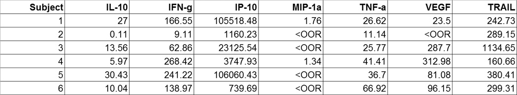

(A), Spreadsheet example of a mismatched data type in a column with the <OOR values. <OOR, out of range, low, meaning below limit of assay detection. (B), Spreadsheet containing missing values, as well as mismatched data types present in columns AF as well as AG.
An analytical data check is performed to detect spurious data types. Data in spreadsheets (tabular data) imported into Microsoft Excel can be analyzed by function checks. One check for numeric values can be performed with the function “IsNumber”; or for character data, the function “IsText” can be used. Most software packages have similar built-in data check functions; for example, “is.numeric” and “is.char” are available in the R software package (http://www.r-project.org/).
A data validity check examines the correctness and reasonablenesss of data. This check looks at the overall range of the values for a given column. If, for example, a certain column should only contain positive values, the minimum value for that column can be calculated to make sure all the entries are a positive value. Similarly, the range of the columns can be examined using built-in software functions. If these exceed the bounds of the expected values, the study investigators should be consulted to resolve the discrepancy.
A graphical analysis is typically done using such methods as scatterplots, boxplots, and quantile-quantile (q-q) plots. Scatterplots allow one variable to be compared against another, or one group of subjects against another (such as a control and a treatment group). Scatterplots are used to identify the presence of trends in the data or outliers in the dataset (Fig. 3). Trends are indicated by the relationship of the data – whether it falls on a straight line, or more complex functions. Outliers are suggested by the existence of data points that lie distinctly away from all others. If it appears that most spots appear to lie along a straight line, this might indicate that the two variables are highly correlated, a finding that is important to note for downstream analysis. If the data has outliers, it is important to discuss with the experimentalists if there is an experimental reason for their presence. Such reasons might include buffer changes, power outages, or different technicians conducting the assay. If there is such a reason for the outlier values, this is evidence that that data might be discarded from the downstream analysis. Outliers may also be the result of accidental errors on spreadsheet entry. If, on the other hand, no reason for the outliers can be found, the outlying data points must be included in the downstream analysis, and subsequent analytical methods need to be modified to properly deal with them.
Fig. 3. Graphical analysis: scatterplots.

Scatterplot showing relationship between IL6 and IL10 Bioplex Cytokine Assay data for patients infected with Dengue Fever (in the raw format). From this plot, one might conclude that the spot at (~125,~20) is an outlier as it is distinctly different from all other values. One would specifically need to check the IL6 value as that seems the one that is different from the others (a value of 20 for the IL10 seems to fit with the others).
Box-plots are useful in graphical analysis for several reasons. Box-plots are representations of the mean (horizontal line), the 25–75% interquartile range (boxed region), and standard deviation (whiskers) of a group of observations (Fig. 4). Box-plots give an analyst information about data symmetry. Symmetry is assessed visually if the mean line lies in the middle of the rectangle (the boxed region representing 50% of the data - the 25–75% interquartile range), and if the tails of the box-plot are also equal in length (meaning the data is distributed equally on both sides of the mean value). Data symmetry is important because certain techniques used in downstream data analysis (such as student’s t-test) assume the data is normally distributed. Box-plots are also useful in outlier detection. Outlier points are frequently denoted with a star, and their identification requires resolution with the experimentalists as described above. Finally, box-plots can be used to compare multiple groups to look for differences or overlap between the various groups. Difference comparison is useful because it gives the analyst an indication where significant differences may be found when performing hypothesis tests. Software programs commonly used for creating box-plots are SAS, SPSS, SigmaPlot and R.
Fig. 4. Graphical analysis: outlier identification.

Box-plots for log2 transformed IL6 and IL10 Bioplex cytokine assay data. DF= Dengue Fever; DHF = Dengue Hemorrhagic fever. This plot indicates that there is an outlier within the Dengue Fever population for IL6 (evidenced by *). This also shows that the DHF subjects do not have symmetric data. This is shown because the median line in their boxplots is not in the center of the colored rectangle, but very near the top of it. The data from the DF subjects appear to possibly be normally distributed as their boxplots appear mostly symmetric, with the outlier possibly being a problem for IL6 and the long tail for IL10 possibly being a problem. Both warrant further examination.
Quantile-quantile plots (q-q plots) are useful for determining whether the data match that of a normally distributed dataset, or if groups of data follow similar distributions. Q-q plots are quantiles of the data along the x-axis, and the quantiles of a randomly generated, normally distributed dataset with the same mean and standard deviation along the y-axis (Fig. 5). Not normally distributed data will not fall along a diagonal line or deviate strongly at both the beginning points and ending points (Fig. 5a,b). This type of figure indicates that the “tails” of the dataset are different from that of a normally distributed dataset. In reality, what that means is that the largest values and the smallest values are different from what is expected with normally distributed data. For normally distributed data, the points on the q-q plot will follow a straight diagonal line through the middle of the graph (Fig. 5c).
Fig. 5. Normality assessment and transformation.


(a), a q-q plot of data that is not normally distributed. It is for DF patients, IL6 raw values. The fact that the shape of the curve formed by the points is not linear, not does it remotely match the straight diagonal both indicate the data is not normally distributed. (b), a q-q plot shows the same dataset, however this time, it has been normalized by a log transformation. Again, this plot indicates that the data is still not normally distributed as there is curvature to the points and they do not match the straight diagonal line well. (c), a q-q plot of normally distributed data. It is log transformed data for DF patients, IL10. The majority of the data points lie along the diagonal line.
5. Preprocessing: missing values and transformation
Missing data is characteristic of high throughput data sets, where observations are not made in every sample, or the analyte concentration is below the limit of detection for a particular assay. The presence of a significant amount of missing data complicates many statistical analytic and machine learning approaches. Imputation is one method for dealing with missing data, where the missing values are substituted based on heuristics or mathematical assumptions. In our dataset, missing values (<OOR, Fig. 2a) were the consequence of the cytokine being below the assay limit of detection. In this case, the simplest and most appropriate method for imputation is based on heuristics, where substitution of <OOR values with a value of 1/10th of the lower limit of detection for each assay. Alternatively, K nearest neighbors (KNN) is a data-driven imputation technique [6] where imputed values are represent those based on their distance between correlated neighbors (KNN implementations are available in R package and Matlab program).
Another issue in data pre-processing is how to treat data that fail analysis of normality, as suggested by box-plot or q-q graphical analysis. This consideration is important because statistical approaches for comparing feature expression in non-normally distributed data requires the use of analytical approaches distinct from standard parametric testing (Fig. 1). Because parametric testing is more powerful, analysts will frequently employ statistical transformations to make the data set behave more like normally distributed data. Popular data transformations include taking the logarithm of the data (log base 10 or natural logarithm) or taking the square root of the data. Generally, if a transformation of a feature in one group is performed, the same transformation should be applied to the feature in other groups of the data set (i.e. if the DF cytokine expression values are transformed, then so should the DHF cytokine values). The transformed data set can then be re-examined for normality using the graphical approaches described above. An example of the effect of log transformation is shown in Fig. 5a and b, where the raw data significantly deviates from the normal distribution (Fig. 5a); after log2 transformation, the data is more closely resembles a normal distribution (Fig. 5b), where parametric statistics are then applied.
6. Feature Reduction
A characteristic of complex, multidimensional data sets is that many features are identified. The curse of dimensionality is a well-known phenomena, where the presence of many features often leads to worse performance of the classifier, rather than better performance. Potential solutions to this problem can include reducing the dimensionality and simplifying the model complexity. Feature reduction is a necessary step before creating a biomarker panel because only the most informative features should be used to create a classification model. A flow diagram is shown in Fig. 6.
Fig. 6. Flow diagram for feature reduction and machine learning.

A schematic for the use of feature reduction and downstream supervised or unsupervised classifications. Abbreviations: CART, classification and regression trees; RF, random forests; SVM, support vector machines; MARS, multivariate adaptive regression splines.
Dimensionality can be reduced by selecting an appropriate subset among the existing features. This can be made by selecting a subset of features that are rank-ordered by statistical significance, by calculating the fold change between the two comparison groups, by a statistical analysis of microarrays, Bayes methods or heuristics. Selection of the feature reduction method is made on the data set characteristics, the goals of the analysis or biological intuition of the investigators (Table I). Statistical based feature reduction often starts by comparing different means either using the two sample t-test or Wilcoxon rank sum test at a given appropriate level of significance. The Wilcoxon rank sum test is an alternative approach to the students t-test in two-sample comparisons without requiring a parametric assumption. Under the general condition that the feature distributions are not highly skewed or have a heavy-tailed distribution, we use a two sample t-test procedure on log-transformed data [7].
Table I.
Feature reduction techniques and selection criteria
| Feature Reduction Technique |
Why Select? | Considerations |
|---|---|---|
| Rank Ordered t-test |
|
|
| Fold change (FC) cut-off |
|
|
| SAM |
|
|
| Empirical Bayesian |
|
|
| PCA |
|
|
| Heuristics |
|
|
Analyzing multidimensional data frequently involves the simultaneous testing of more than one hypothesis, a procedure that leads to inflated numbers of false positives. Common methods for reducing false positives, called multiple hypothesis testing, are family-wise error rate corrections such as the Bonferroni correction and the false discovery rate (FDR). FDR procedures using a re-sampling method have improved ability to reject false hypotheses compared to the more conservative Bonferroni correction [8]. When a feature is called significant, it signifies the quantile (q)-value is below that value indicating the minimum acceptable FDR, an estimate of the proportion of false positives. For example, if a feature has a q-value of 0.05, it means that 5% of features that show p-values at least as small as that are false positives. Feature reduction can also be based on a fold change value (values of 1.5 or 2 are often used) or statistical significance of mean difference of two groups (a q-value threshold of 1% or 5% are often used). The fold change threshold will change the number of significant features when the analysis is followed by the use of a parametric test with multiple testing corrections.
Significance analysis of microarrays (SAM) is a widely used permutation-based approach to identifying differentially expressed features in high dimensional datasets. One of the advantages of SAM is that it is able to assess statistical significance using FDR adjustment [9]. In the SAM analysis, each feature is assigned a score on the basis of its change relative to the standard deviation of its repeated measurements. SAM accounts for feature-specific fluctuations in signals, and adjusts for increasing variation in features with low signal-to-noise ratios. Data are presented as a scatter plot of expected versus observed relative differences, where significant deviations that exceed a threshold from expected relative differences are identified and considered “significant”. The Microsoft Excel add-in SAM package can be used with specific option filtering. There are several options, for example, multi-class, two class paired, and two class unpaired response types using the t-test, Wilcoxon test, and analysis of variance test (Table I).
An alternative approach for feature reduction is an empirical Bayesian technique [10]. This approach uses non-informative priors and derives the posterior probability difference for each predictor. An advantage of empirical Bayes is that it does not rely on initial feature selection using t-tests or Wilcoxon tests to identify which features are differentially expressed. However, there are limited software implementations of this method and it requires significant computational time [11]. Software implementations are R or Winbugs.
Principal component analysis (PCA) is a method for reducing the dimensionality of data to identify informative features. Here, features are transformed into orthogonal linear representation to identify uncorrelated components that most contribute to the variability in the experimental data. The features employed in the major principal components are then used in order of the magnitude of their corresponding eigenvalues.
Finally, intuition of the biological system (heuristics) can be used to select features based on their plausibility or prior knowledge about the system under investigation. Heuristics is a method which is frequently used in combination with various statistical methods (Table I). in practice, several feature selection methods are applied to identify a subset of differentially-expressed predictors that are useful and relevant for distinguishing different classes of samples.
7. Unsupervised Learning
Unsupervised learning seeks to identify hidden structures in a data set without regard for the individual outcome. There are several different algorithms that fall under the category of unsupervised learning. These include hierarchical clustering, k-means clustering, and principal components analysis (PCA).
Hierarchical clustering seeks to group available data into clusters by the formation of a dendrogram or tree [12]. The ultimate thought is that members of each cluster are more closely related to other members of that cluster than they are to members of another cluster. The process by which samples are grouped into clusters is determined by a measure of similarlity between the objects. Various measures of similarity exist which include Euclidean distance, Manhattan (city-block) distance, and Pearson correlation. Not only similarity (distance) between two data points measured, but the distance between two clusters is measured. This distance can be calculated in three different ways: 1) the minimum distance between any two objects in the different clusters; 2) the maximum distance between any two objects in the different clusters; and 3) the average distance between all objects in one cluster and all objects in the other cluster. In addition to measures of similarity and distance, one can build the dendogram either via top-down (divisive) methods or bottom-up (agglomerative) methods.
For divisive methods, the process starts with every object belonging to a single cluster. Then, the process is a recursive one in which one large cluster is divided into two separate ones that are the most dissimilar from each other. This process is repeated until every object belongs to its own cluster. For agglomerative methods, the process starts with each object belonging to its own cluster. Next, the two most similar objects are grouped together into their own cluster. The process recursively continues grouping the most similar objects/clusters together until every object is contained within a single cluster.
K-means clustering seeks to group objects into k clusters, where k is some predetermined number [13]. The distance/similarity metric used in k-means clustering is the Euclidean distance. The algorithm starts by first deciding at random the locations for the centers of k clusters. Each object in the cluster is assigned with the closest mean, as determined by the Euclidean distance from that object to the cluster center. The cluster centers are then recalculated using the objects within the cluster, and the assignment process is repeated. This iterative process continues until the assignments of objects to clusters no longer changes.
Principal component analysis (PCA) is useful for the classification as well as dimension reduction (compression) of a dataset. The main goal of PCA is to find a new set of variables, called principal components, that represent the majority of the information present within the original dataset. The information is related to the variation present within the original dataset, and is calculated by the correlation between the original variables. The number of principal components is smaller than the initial number of variables in the dataset. The identification of his new variable space will reduce the complexity and noise within the dataset and reveal hidden characteristics within the data. The principal components are uncorrelated (orthogonal) with each other and are also ordered by the total fraction of information about the original dataset they contain. The first principal component accounts for as much of the variability in the original dataset as possible, and each subsequent component accounts for as much of the remaining variability as possible. In a reliable PCA, the first 3 principal components should account for at least 85% of the total variation within the dataset. If this value is less than 80% of the total variation, PCA is not the preferred method of analysis. The process for determining the principal components is one based on eigen vectors and eigen values after mean centering each variable. The results are presented in the form of scores and loadings. Scores are the transformed data values that correspond to each original variables, and loadings are the weight by which each mean centered original variable should be multiplied by in order to obtain the score.
8. Classification by machine learning
Machine learning is the study of how to build systems that learn from experience. It is a subfield of artificial intelligence and utilizes theory from cognitive science, information theory, and probability theory. Machine learning usually involves a training set of data as well as a test set of data. Frequently the training and test data are both taken from the same dataset, and the system is “trained” using the training data, and then run on the test data to classify it. Machine learning has recently been applied in the areas of medical diagnosis, bioinformatics, stock market analysis, classifying DNA sequences, speech recognition, and object recognition. More applications are expected to be developed in the near future.
As the goal of this paper is to compare/contrast several different classification algorithms, we compare the results of the various methods using the dengue fever dataset that has had featured reduction methods applied to it as described above. The same dataset was used in all methods.
8.1 Supervised Classification
Supervised clustering is a type of data analysis where one seeks to create clusters within the data, or more to the point, one seeks to make a prediction about the data based upon some set of input variables. The input variables are used to make some prediction about the outcome. Supervised clustering is distinguished from unsupervised clustering in that for supervised clustering, the “truth” must be known in order to train the model. In the case of the DF study, we are using a set of predictor variables to ultimately decide whether a patient has DF or the more severe DHF.
In machine learning, one typically divides the available data into a training dataset and a testing dataset. The training dataset is simply a subset of the entire dataset which will be used to “train” or build the classification model. The training dataset, then, is the remaining subset of the original data that will be used to “test” or check the classification model for accuracy on another portion of the data. If 100 or more samples are found within the dataset, creating a training and testing set is optimal. However, frequently the sample sizes are much smaller in “omics” studies. How then should one create testing and training set? The answer is to instead use cross-validation (CV), a technique widel employed to give an accurate indication of how well an algorithm is able to make new predictions. CV is appropriate for each of the classification methods discussed below. The simplest CV approach is the “holdout method” that splits the data into two sets – a training set and a test set. From a full dataset of samples for which the outcome is known, half the members are randomly selected and placed in the “training set”; the other half are designated as the “test set”. For example, SVM would be run on the training data to create a candidate classifier which is then used to predict the outcomes for the test data. CV then uses the prediction errors to estimate the accuracy of the classifier in matching the known outcomes of the test set. Unfortunately, this evaluation can be highly variable because it is dependent upon which data elements were selected to be in the training set versus the test set.
One improvement on the holdout method that addresses this deficiency is k-fold CV. In k-fold CV, the full dataset is divided into k subsets and the holdout method is repeated k times. Each time, one of the k subsets is used as the test set and the remaining subsets are used as the training sets. The average error across all trials is then computed to assess the predictive power of the classification technique used. The advantage of the k-fold CV method over the holdout method is that by comparing the results of many training set versus test set trials to calculate an average predictive error, it arrives at an estimate of the predictive power of the algorithm that is much less dependent upon the initial selection of members for the training set. A common choice for k is 10. Because feature reduction techniques are utilized before machine learning algorithms are run, using CV does not prohibitively or significantly increase the algorithm run time.
8.2 Logistic Regression
Logistic Regression is the simplest form of supervised clustering, and although not typically considered a form of machine learning, it is widely used in supervised classification problems. Its main objective is to model the relationship between a set of continuous, categorical, or dichotomous variables and a dichotomous outcome which is modeled via the logit function. Whereas typical linear regression seeks to regress one variable onto another (typically continuous data), logistic regression seeks to model via a probability function called the logit a binary outcome. A logistic regression equation takes the form:
| (1) |
, where p is the probability that event Y occurs P(Y=1), p/(1−p) is the odds ratio, ln[p/(1−p)] is the log odds ratio (the logit), βi are constants, and M is the number of predictors.
Thus, logistic regression is the method used for a binary, rather than a continuous outcome. The logistic regression model does not necessarily require the assumptions of some other regression models, like assuming that the variables are normally distributed in linear discriminant analysis. Maximum likelihood estimation is the method used to solve for the logistic regression equation. Recent techniques, penalized shrinkage and regularization estimation, least absolute shrinkage and selection operator (LASSO) type regularization are innovative logistic regression models for simultaneous variable selection and coefficient estimation. Their application improve logistic regression prediction accuracy in classification [8].
8.3 Classification and Regression Trees (CART)
CART is a non-parametric modeling algorithm for building decision trees using the methodology developed for building phylogenetic trees [14]. Decision trees have a human-readable split at each node which is a binary response of some feature in the data set. CART performs binary recursive partitioning that classifies objects by selecting from a large number of variables the most important ones in determining the outcome variable. CART is highly useful for our applications because it does not require initial variable selection. Some of the advantages of CART are that it can easily handle data sets which are complex in structure, it is extremely robust and not very effected by outliers, and it can use a combination of both categorical and continuous data. Another advantage of CART is that missing data values do not pose an obstacle to CART classification because the algorithm develops alternative splits which can be used to classify the data when there are missing values (Table II).
Table II.
Machine learning approaches to supervised classification.
| Algorithm | Advantages | Disadvantages |
|---|---|---|
| CART |
|
|
| Random Forests |
|
|
| MARS |
|
|
| SVM |
|
|
| Logistic Regression |
|
|
The three main components of CART modeling are creating a set of rules for splitting each node in a tree, deciding when a tree is fully grown, and assigning a classification to each terminal node of the tree [14]. The basic algorithm for building the decision tree seeks some feature of the data which splits it maximizes the difference between the classes contained in the parent node. CART is a recursive algorithm which means that once it has decided on an appropriate split resulting in two child nodes, the child nodes then become the new parent nodes, and the process is carried on down the branches of the tree. CART uses CV to determine the accuracy of the decision trees.
8.4 Random Forests (RFs)
RFs improve upon classical CART decision trees while still keeping many of the most appealing properties of tree methods (Table II). Decision trees are known for their ability to select the most informative descriptors among many and to ignore the irrelevant ones. RF offer several unique and extremely useful features which include built-in estimation of prediction accuracy, measures of feature importance, and a measure of similarity between sample inputs [15]. By being an ensemble of trees, RF inherits this attractive property and exploits the statistical power of ensembles. The RF algorithm is very efficient, especially when the number of descriptors is very large. This efficiency over traditional CART methods arises from two general areas: The first is that CART requires some amount of pruning of the tree to reach optimal prediction strength; RF, however, does not do any pruning, which reduces performance time. Secondly, RF uses only a small number of descriptors to test the splitting performance at each node instead of doing an exhaustive search as does CART.
RF thus builds many trees and determines the most likely splits based upon a comparison within the ensemble of trees. The RF modeling uses first a bootstrapped sample from the training dataset. Then, for each bootstrapped sample, a classification tree is grown. Here, RF modifies the CART algorithm by randomly selecting from a subset of the descriptors, instead of choosing the best split among all samples. This procedure is repeated until a sufficiently large number of trees have been computed, usually 500 or more.
In practice, some form of cross-validation technique is used to test the prediction accuracy of any computational technique. RF performs a bootstrapping cross-validation procedure in parallel with the training step of its algorithm. This method allows some of the data to be left out at each step, and then used later to estimate the accuracy of the classifier after each instance (i.e. tree) has been completed.
8.5 Multivariate Adaptive Regression Splines (MARS)
MARS is a robust nonparametric modeling approach for feature reduction and model building [16]. MARS is a nonparametric, multivariate regression method that can estimate complex nonlinear relationships by a series of spline functions of the predictor variables. Regression splines seek to find thresholds and breaks in relationships between variables and are very well suited for identifying changes in the behavior of individuals or processes over time (Fig. 7a). Some of the advantages of MARS are that it can model predictor variables of many forms, whether continuous or categorical, and it can tolerate large numbers of input predictor variables. As a nonparametric approach, MARS does not make any underlying assumptions about the data distribution of the predictor variables of interest. This characteristic is extremely important in modeling DHF because many of the cytokine and protein expression values are not normally distributed, as would be required for the application of classical modeling techniques such as logistic regression. The basic concept behind spline models is to model using potentially discrete linear or nonlinear functions of any analyte over differing intervals. The resulting piecewise curve, referred to as a spline, is represented by basis functions within the model.
Fig. 7. MARS modelling of DHF.


(a) Schematic view of MARS model development. Features selected from clinical laboratory, cytokine and proteomic analyses were used to develop classifier for DHF outcome. For each analyte selected, a basis function is developed where changes in the concentration of that basis function is related to clinical outcome. (b) Analysis of features in DHF MARS model. Variable importance was computed for each feature in the MARS model. Y axis, percent contribution for each analyte.
MARS builds models of the form:
| (2) |
Each basis function BFi(x) takes one of the following three forms: 1) a constant, where there is just one such term, the intercept; 2) a hinge function. A hinge function has the form max(0,xi − ci) or max(0,ci − xi). MARS automatically selects variables and values of those variables for knots of the hinge functions; or, 3) a product of two or more hinge functions. These basis functions can model interaction between two or more variables.
The MARS algorithm has the ability to search through a large number of candidate predictor variables to determine those most relevant to the classification model. The specific variables to use and their exact parameters are identified by an intensive search procedure that is fast in comparison to other methods. The optimal functional form for the variables in the model is based on regression splines called basis functions. MARS uses a two-stage process for constructing the optimal classification model. The first half of the process involves creating an overly large model by adding basis functions that represent either single variable transformations or multivariate interaction terms. The model becomes more flexible and complex as additional basis functions are added. The process is complete when a user-specified number of basis functions have been added. In the second stage, MARS deletes basis functions in order of least contribution to the model until the optimum one is reached. By allowing for the model to take on many forms as well as interactions, MARS is able to reliably track the very complex data structures that are often present in high-dimensional data. By doing so, MARS effectively reveals important data patterns and relationships that other models often struggle to detect. Missing values are not a problem because they are dealt with via nested variable techniques. CV is used within MARS to avoid over-fitting the classification model, and randomly selected test data can also be used to avoid the issue as well. The end result is a classification model based on single variables and interaction terms which will optimally determine class identity. Thus, MARS excels at finding thresholds and breaks in relationships between variables and as such is very well suited for identifying changes in the behavior of individuals or processes over time. Software implementation of MARS is available in R or from commercial vendors (Salford Systems).
There are several parameters within the MARS framework that can be adjusted. From experience, we have learned that 10-fold CV is ideal, in modeling applications where the sample size is small. In addition, the only other parameter that needs adjusting is the maximum number of basis functions. The default is 15, and based on recommendations from the original MARS paper, this number should be changed to 3 times the number of parameters intended to appear in the final model [16].
8.6 Support Vector Machines
Support vector machines are based on simple ideas that originated in the area of statistical learning theory [17]. The simplicity arises from the fact that SVMs apply a transformation to highly dimensional data to enable researchers to linearly separate the various features and classes. Luckily, the data transformation allows researchers to avoid calculations in high dimensional space. The popularity of SVMs owes much to the simplicity of the transformation as well as their ability to handle complex classification and regression problems. SVMs are trained with a learning algorithm from optimization theory and tested on the remainder of the available data that were not part of the training dataset [18, 19]. The main aim of SVMs is to devise a computationally effective way of learning optimal separating parameters for two classes of data.
SVMs use an implicit mapping of the input data, commonly referred to as Φ, into a highly dimensional feature space defined by some kernel function. The learning then occurs in the feature space, and the data points appear in dot products with other data points [20]. One particularly nice property of SVMs is that once a kernel function has been selected and validated, it is possible to work in spaces of any dimension. Thus, it is easy to add new data into the formulation since the complexity of the problem will not be increased by doing so.
There are a few decisions that need to be made when working with SVMs. Namely, a method for data preprocessing must be identified (we recommend the method of Z-scoring- e.g., subtracting the mean and dividing by the standard deviation), what format to use for the kernel function, as well as choosing the parameters for the kernel function. Kernel choices include a linear kernel, a quadratic kernel, a radial basis function, or a sigmoidal kernel. In practice, we evaluate several. For bioinformatics applications where the sample size is relatively small (fewer than 100 samples) and the variable space is rather large (more than 30 variables), we have found that the linear kernel works fairly well. The linear kernel is advantageous because there is only one parameter (C) that needs to be optimized, so an exhaustive search can be performed to optimize it. If the fit of the linear kernel is not ideal, we suggest trying a radial basis function instead. We use the C value estimated from the linear kernel as a baseline for the C value in the radial basis function kernel. Unlike the linear kernel, however, with a radial basis function kernel, an additional parameter, γ, needs to be optimized. An exhaustive search to optimize parameters is frequently not plausible due to time constraints, so a grid-search is frequently employed to optimize the parameters. To do this, grid points on a logarithmic scale are chosen for both parameters, and the SVM algorithm is run. The accuracy can then be estimated for all grid points. The optimized parameters are those that provide the best classifier accuracy.
8.7 Additional Methods
Several methods are rapidly emerging in the literature as viable options for predictive modeling. Among these are various ensemble methods made popular by Giovanni Seni, John Elder and Leo Breiman [21, 22]. Ensemble methods use multiple different models/techniques to obtain a model with better predictive performance than any single model on its own. Popular ensemble methods include Bayesian model averaging, Bagging [22], Random Forests [23], Adaboost [24], and Gradient Boosting [25, 26]. Other emerging techniques including creating hybrid models which involve using the results of one modeling as input into another. One such hybrid involves using the basis function results from a MARS analysis as input parameters for a generalized linear model, referred to as MARS-logit hybrid modeling [27]. These models are useful for modeling feature interactions, and provide approaches to probabilitistic determination of nonparametric relationships.
9. Model Diagnostics
Model diagnostics is an important procedure to assess model adequacy for algorithmic procedures within a machine learning framework. In multiple linear or logistic regression, often the interest is to assess the linear or non-linear association of binary responses on covariates. A logistic regression model assumes that the logit of the outcome is a linear combination of predictors. If the model assumptions are not satisfied, the model may contain biased coefficient estimators and very large standard errors for regression coefficients.
In practice, we perform regression modeling and examine on a post-hoc basis whether all relevant predictors of our model maintain the appropriate linear association with outcome. One method for assessing this relationship is to use Generalized Additive Models (GAMs). GAMs are regression models which can evaluate complex non-linear predictors on the outcomes in a generalized linear model setting [28]. A GAM plot is represented by the value of the covariate (feature) on the X-axis, and the partial residual represent the difference between the estimated- and observed value on the Y-axis (Fig. 8). The relationship of the covariate with the outcome is indicated by a smoothed piecewise polynomial relationship contained within 95% confidence limits. We evaluate the partial residual plot as a diagnostic graphical tool for identifying nonlinear relationships between the response variable and covariates for generalized additive models. In the case of the albumin covariate, the piecewise polynomial relationship is not a linear relationship, and therefore albumin would require a nonparametric modeling approach (Fig. 8a). By contrast, tropomyosin has a linear relationship and parametric (logistic) modeling would be justified. For each covariate, we also will examine the log-likelihood ratio test p-values by comparing the deviance between the full model and the model without that variable. The projection (hat) matrix and Cook's distance are used to evaluate the effect of outliers and influential points on the model [29].
Fig. 8. Generalized Additive Models.


For each graph, the Y axis is the partial residual and the X axis is the value of the covariate (feature). Dashed lines are 95% confidence intervals. Open circles are data points. (a), Partial regressions for albumin in DHF prediction demonstrating a nonparametric relationship with outcome. (b), Partial regressions for tropomyosin in DHF prediction demonstrating a global linear relationship with outcome.
For machine learning algorithms such as SVMs, CART, or MARS, model performance can be examined using a confusion matrix. A confusion matrix shows the actual number of cases within each group, as well as the number of cases predicted by the model to lie within each group. This analysis allows the modeler to determine model performance for prediction of each class. In addition, the overall percent correct prediction is also evaluated. An example of the confusion matrix for the Dengue Fever study is shown in Table III. The MARS model predicts both the DF and DHF cases with 100% accuracy.
Table III. Confusion matrix for MARS classifier of DHF.
For each disease (class), the prediction success of the MARS classifier is shown. Reprinted with permission from [2].
| Class | Total | Prediction | |
|---|---|---|---|
| DF (n=38) |
DHF (n=13) |
||
| DF | 38 | 38 | 0 |
| DHF | 13 | 0 | 13 |
| Total | 51 | correct =100% | correct =100% |
Finally, we use both change in residual deviance in parametric or nonparametric models, and the area under the receiver operating characteristic (ROC) curve for comparison of the performance of the statistical models. The area under the ROC curve (AUC) measures indicate the ability of a model to discriminate amongst the outcome groups. An AUC score of 0.5 indicates that a model has no discriminatory ability and a score of 1 indicates the two groups are perfectly discriminated. In Fig. 9, we illustrate the use of the ROC to compare model performance of different logistic models in prediction of DHF. In this example, we performed logistic modeling using simple clinical features that satisfied a parametric modeling approach [3]. Models 1–3 are logistic regression models based on best subset selection having the top ranked three largest score statistics to differentiate the binary outcome among all three candidates among all predictors. Model 4 is the ROC for the MARS model (Fig. 7). Note that the ROC curves are all significantly leftward shifted from the line of no discrimination, indicating that all models perform better than random guessing. However, the AUC of Model 4 is significantly higher than the other three logistic regression models, indicating that the prediction performance of MARS modeling is better in this data set.
Fig. 9. Receiver operating characteristic curve.

Shown is an example of ROC curves for four different models of the Dengue Fever data set. Model 1 : Logistic regression of Platelets, IL10, Lymphpocytes; Model 2 : Logistic regression of Platelets, Il10, Neutrophils; Model 3: Logistic regression of Platelets, IL10 and IL6; Model 4, MARS.
10. Model Performance
An example of the use of MARS in supervised classification is provided from the DF study. The results of the data exploration indicated that proteomic quantifications violated normal distributions, and included outliers, suggesting that nonparametric modeling methods were justified. To build the MARS model, the patient’s gender, logarithm-transformed cytokine expression values (IL-6 and IL-10), and 34 2DE protein spots were modeled using 10-fold CV and a maximum of 126 basis functions. The optimal model was selected on the basis of the lowest generalized cross-validation error. The features retained in the optimal model were 1 cytokine (IL-10) and 7 protein spots. The optimal MARS model is represented by a linear combination of 9 basis functions, whose values are shown in Table IV. Also of note, the basis functions are composed of single features, indicating that interactions between the features do not contribute significantly to the discrimination. To determine which of these features contribute the most information to the model, variable importance was assessed. Variable importance is a relative indicator (from 0–100%) for the contribution of each variable to the overall performance of the model (Fig. 7b). The variable importance computed for the top three proteins was IL-10 (100%), with Albumin*1 (50%) followed by fibrinogen (40%). These numbers indicate each feature’s relative importance for model performance (accuracy in cross-validation). The overall accuracy for this model is 100%, with an AUC of 1. Fig. 10 shows the ROC curves for all the models mentioned in this section.
Table IV. MARS Basis Functions.
Shown are the basis functions (BF) for the MARS model for Dengue hemorrhagic fever. Bm, each individual basis function, am, coefficient of the basis function. (y)+, = max(0,y).
| Bm | Definition | am | Variable descriptor |
|---|---|---|---|
| BF1 | (IL-10 −1.15)+ | 5.83E-03 | IL-10 |
| BF3 | (20873 – Fibrinogen)+ | 5.42E-05 | Fibrinogen |
| BF5 | (437613 - Albumin)+ | 1.39E-06 | Albumin*1 |
| BF6 | (C4A – 385932)+ | −4.90E-06 | Complement 4A |
| BF8 | (C4A – 256959)+ | 3.25E-06 | Complement 4A |
| BF11 | (469259 – Albumin)+ | 2.48E-06 | Albumin*2 |
| BF17 | (122218 – TPM4)+ | 5.27E-06 | TPM4 |
| BF19 | (immunoglobulin gamma - 57130)+ | −1.35E-06 | Immunoglobulin gamma-chain, V region |
| BF23 | (657432 – Albumin)+ | −9.97E-07 | Albumin*3 |
Variable isoforms likely due to post-translational modification and/or proteolysis.
Reprinted with permission [2].
Fig. 10. Receiver operating characteristic curve for fitted models.

Shown are the ROC curves for four different models of the Dengue Fever data set. MARS, CART, and SVM all had the same curve, displayed by the continuious line. Random Forests had a poorer performing AUC as indicated by the dashed line.
The same DF study input data was used with CART for comparison purposes. In CART, the default size of the parent node was changed to 10 instead of 5 due do the small sample size of this study. 10-fold CV was used as well since the sample size was too small to consider both a training and testing dataset. The seven nodes that appeared in the final model contained splits that were based upon IL-10, IL-6, TPM4- ALK fusion oncoprotein type 2, Albumin, and two other proteins. As one can easily deduce, several of the variables chosen for the splits in the CART model are different from those used by the basis functions that appear in the MARS model. The overall AUC for the CART model was 1.0 as well (see Fig. 10), and the CART model had an accuracy of 100%. It should be noted that the variables with the highest importance for the CART model were also IL-10 (100%) and Albumin*1 (86%), suggesting that both models identify IL-10 and Albumin*1 are the most important discriminative features.
In addition, the same DF study input data was used with both RF and well as SVM methods. For RF, out of bag was used for testing because CV is not an option. The default number of predictors at each node was increased from 3 to 5 since the study is small, and computational time was not an issue. In addition, for RF, the default number of parent nodes was changed to 2 based on a recommendation from the algorithm. The overall accuracy for RF was only 86%, indicating that in this instance, RF does not out-perform CART. The AUC for RF was only .87 (Fig. 10). The model was able to classify correctly all DF outcomes, but had much more difficulty with the DHF outcomes and was only able to correctly classify 6 of 13 cases. The one commonality between RF and the CART and MARS models is that IL-10 was still the most important variable within the model. In order to run SVM, we had to standardize the data by transforming it to be between 0 and 1. This was accomplished by Z-score transformation (subtracting the group mean and dividing by the standard deviation). Since SVM is a “black box” algorithm, nothing is known about which variables influence the model selection. Instead, all that can be gleaned from the SVM model is the overall performance and the AUC. For the DF data, we chose to run an SVM model using a radial basis function as our kernel. This is because the GAM analysis indicated that a linear fit might not be best for our data. For SVM, the overall accuracy was 90%; all DF patients were accurately classified, but only 8 of the 13 DHF patients were correctly classified by SVM. The AUC was still 1.00 however (Fig. 10).
11. Reproducibility
Confounding errors, such as those produced by biases in experimental measurements, can result in significant interpretation artifacts [30]. The reliance on automated data analysis pipelines and undocumented analysis steps makes independent scientific replication of a published analysis difficult. Analytic errors can be difficult to identify in complex data analysis plans. Recent difficulties encountered with the re-analysis of complex “omics” data sets has led to the recommendations that raw data, source codes, descriptions of non-scriptable analysis steps and pre-specified analysis plans should all be supplied with any publications [31], particularly those signatures or markers that are to be used as guides to clinical trials or treatments.
As this movement gains acceptance, documenting statistical analysis plans will become increasingly important. Programs in R, such as Sweave, allow dynamic linkage of data and external R files that enable independent scientists to examine all steps of the data analyses, thereby making research more transparent and reproducible to others.
12. Lessons learned
The analysis of complex multidimensional data sets is not trivial, and multiple errors of omission or commission can influence the quality of the analysis and its reproducibility. We suggest that applying a structured approach to data set analysis will result in more robust and consistent analyses, and correct interpretation of these data. In this manuscript, we present our approach for a structured analysis for the benefit of analysts who are new to the problem of analyzing wide (large p, small n) data. Additionally, we cannot overemphasize that a close collaborative interaction between the analyst and experimentalist can significantly improve the efficiency and quality of the result.
In complex data, in addition to the major goal of the analysis, the underlying data structure drives the application of statistical and machine learning tools that would be appropriate to use. For example, selection of an appropriate type of imputation of missing data is driven by an understanding of why these data are missing from the data set. Moreover, the early detection of non-normally distributed data would be important to guide the selection of transformation techniques, or the use of non-parametric statistical comparisons.
Our experience, shared by others in the omics field, is that high-dimensional data sets are composed of a small set of informative features among many uninformative features. These uninformative features mask the information in the data set when the entire data set for machine learning. This process results in poorly performing classifiers that do not generalize well. The incorporation of a feature reduction step is therefore critical for the development of accurate classifiers. Currently, there is no consensus on which feature reduction step would be most appropriate for an individual data structure; in practice we apply several approaches and evaluate the performance of the downstream classifier. More research will be needed to identify the most appropriate methods for feature reduction in high dimensional data sets.
Although the production of a model is a major milestone of a complex classification experiment, we should emphasize that this is not the end of the analytical evaluation. We contend that a careful post-hoc diagnostic of the features and model performance should be undertaken. The goal of this process is to identify any characteristics of features or modeling assumptions that would make the classifier unstable or not generalize well. We have found that the information from the GAM partial residual analysis helps to evaluate whether global linear (logistic) or nonparametric modeling is the most appropriate for the features selected. Although in our experience, the nonparametric MARS modeling performs better than logistic modeling [2, 32], there are important disadvantages to the nonparametric approach. For example, nonparametric modeling will not result in identification of probabilities of an outcome, a feature that is useful for biomarker panels to be employed clinically. Another limitation is that MARS does not detect co-linear features. As a result, co-linear features may be present in the models that may reduce its performance in independent samples. Post-hoc analyses of feature correlations in the final MARS model will indicate whether multi-colinearity needs to be considered. More research will be needed in hybrid or ensemble methods to produce classifiers for other data types.
The challenge of model selection is selecting the best model that generalizes well given the data. Because the data structure (and therefore optimal modeling approach) is not known a priori, in practice we develop classification models using several feature sets and modeling approaches in parallel. In this example, we use cross-validation, an iterative approach of using a portion of the data to train a given model, and then compare the model developed on the test data set. The cross-validation approach is used in situations where limited data is available (ideally, model validation should be performed on a completely independent data set to evaluate the model’s real-world performance). By post-hoc analysis of the major features retained in each model, comparing their performance using ROC and confusion matrices, and applying prior biological knowledge, the most appropriate models can be selected.
Acknowledgements
This research was supported by the NIAID Clinical Proteomics Center, HHSN272200800048C (ARB), NIH-NHLBI-HHSN268201000037C NHLBI Proteomics Center for Airway Inflammation (ARB), and the Clinical and Translational Science Award (UL1TR000071) from the National Center for Advancing Translational Sciences, NIH (ARB).
Abbreviations
- AUC
Area Under the Curve
- BF
basis functions
- CART
classification and regression trees
- CV
cross validation
- DF
dengue fever
- DHF
dengue hemorrhagic fever
- FC
fold change (of group mean)
- FDR
false discovery rate
- LASSO
least absolute shrinkage and selection operator
- MARS
multivariate adaptive regression splines
- q-q
quantile-quantile
- RF
random forests
- ROC
receiver operating characteristic
- SAM
significance analysis of microarrays
- SVM
support vector machines
Footnotes
Publisher's Disclaimer: This is a PDF file of an unedited manuscript that has been accepted for publication. As a service to our customers we are providing this early version of the manuscript. The manuscript will undergo copyediting, typesetting, and review of the resulting proof before it is published in its final citable form. Please note that during the production process errors may be discovered which could affect the content, and all legal disclaimers that apply to the journal pertain.
Conflict of interest
The authors declare no conflict of interest
References
- 1.Baraniuk RG. More is less: signal processing and the data deluge. Science. 2011;331:717–719. doi: 10.1126/science.1197448. [DOI] [PubMed] [Google Scholar]
- 2.Brasier AR, Garcia J, Wiktorowicz JE, Spratt H, Comach G, Ju H, Recinos A, III, Soman KV, Forshey BM, Halsey ES, et al. A Candidate Biomarker Panel For Predicting Dengue Hemorrhagic Fever Using Discovery Proteomics And Nonparametric Modeling. Clinical and Translational Science. 2011;5:8–20. doi: 10.1111/j.1752-8062.2011.00377.x. [DOI] [PMC free article] [PubMed] [Google Scholar]
- 3.Brasier AR, Ju H, Garcia J, Spratt H, Victor SS, Forshey BM, Halsey ES, Comach G, Sierra G, Blair PJ, et al. A Three-Component Biomarker Panel For Prediction Of Dengue Hemorrhagic Fever. American Journal of Tropical Medicine and Hygiene. 2011 doi: 10.4269/ajtmh.2012.11-0469. in press. [DOI] [PMC free article] [PubMed] [Google Scholar]
- 4.Forshey BM, Guevara C, Laguna-Torres VA, Cespedes M, Vargas J, Gianella A, Vallejo E, Madrid C, Aguayo N, Gotuzzo E, et al. Arboviral etiologies of acute febrile illnesses in Western South America, 2000–2007. PLoS Negl Trop Dis. 2010;4:e787. doi: 10.1371/journal.pntd.0000787. [DOI] [PMC free article] [PubMed] [Google Scholar]
- 5.World Health O. Geneva, Switzerland: World Health Organization; 2009. Dengue: guidelines for diagnosis, treatment, prevention and control. [PubMed] [Google Scholar]
- 6.Troyanskaya O, Cantor M, Sherlock G, Brown P, Hastie T, Tibshirani R, Botstein D, Altman RB. Missing value estimation methods for DNA microarrays. Bioinformatics. 2001;17:520–525. doi: 10.1093/bioinformatics/17.6.520. [DOI] [PubMed] [Google Scholar]
- 7.Always log spot intensities and ratio. [ http://www.stat.berkeley.edu/users/terry/zarray/Htm/log.html]
- 8.Hastie T, Tibshirani R, Friedman A. The Elements of Statistical Learning: Data Mining, Inference, and Prediction. vol. 2. New York: Springer; 2009. [Google Scholar]
- 9.Tusher VG, Tibshirani R, Chu G. Significance analysis of microarrays applied to the ionizing radiation response. Proc Natl Acad Sci U S A. 2001;98:5116–5121. doi: 10.1073/pnas.091062498. [DOI] [PMC free article] [PubMed] [Google Scholar]
- 10.Efron B, Tibshirani R, Storey JD, Tusher V. Empirical Bayes analysis of a microarray experiment. Journal of the American Statistical Association. 2001;96:1151–1160. [Google Scholar]
- 11.Ebayprog.R. [ http://www-stat.stanford.edu/~ckirby/brad/papers/Ebayprogs.R]
- 12.Ben Dor A, Shamir R, Yakhini Z. Clustering gene expression patterns. Journal of Computational Biology. 1999;6:281–297. doi: 10.1089/106652799318274. [DOI] [PubMed] [Google Scholar]
- 13.Lloyd SP. Least squares quantization in PCM. IEEE Transactions on Information Theory. 1982;28:129–137. [Google Scholar]
- 14.Steinberg D, Colla P. CART classification and regression trees. San Diego, CA: Salford Systems; 1997. [Google Scholar]
- 15.Breiman L. Random Forests. Machine Learning. 2001;45:525–531. [Google Scholar]
- 16.Friedman JH. Multivariate Adaptive Regression Splines. Annals of Statistics. 1991;19:1–67. [Google Scholar]
- 17.Karatzoglou A, Meyer D, Hornik K. Support Vector Machines in R. J Stat Softw. 2006;15 [Google Scholar]
- 18.Cristianini N. Large margin strategies in machine learning; Iscas 2000: Ieee International Symposium on Circuits and Systems - Proceedings, Vol Ii; 2000. pp. 753–756. [Google Scholar]
- 19.Cristianini N, Shawe T. Support Vector Machines and other kernel based learning methods. Cambridge, UK: Cambridge University Press; 2000. [Google Scholar]
- 20.Scholkopf B, Smola AJ. A short introduction to learning with kernels. Advanced Lectures on Machine Learning. 2002;2600:41–64. [Google Scholar]
- 21.Seni G, Elder J. Ensemble Methods in Data Mining: Improving Accuracy Through Coming Predictions. San Francisco, CA: Morgan and Claypool Publishers; 2010. [Google Scholar]
- 22.Breiman L. Bagging predictors. Machine Learning. 1996;24:123–140. [Google Scholar]
- 23.Breiman L. Random Forests, random features. Berkeley, CA: University of California; 2001. [Google Scholar]
- 24.Freund Y, Shapire RE. Experiments with a new boosting algorithm; Machine Learning: Proceedings of the 13th International Conference; 1996. pp. 148–156. [Google Scholar]
- 25.Friedman JH. Stochastic gradient boosting. Palo Alto, CA: Stanford University; 1999. [Google Scholar]
- 26.Friedman JH. Greedy function approximation: A gradient boosting machine. Annals of Statistics. 2001;29:1189–1232. [Google Scholar]
- 27.Cook NR, Zee RYL, Ridker PM. Tree and spline based association of gene-gene interaction models for ischemic stroke. Statistics in Medicine. 2005;23:1439–1453. doi: 10.1002/sim.1749. [DOI] [PubMed] [Google Scholar]
- 28.Hastie T, Tibshirani R. Generalized additive models for medical research. StatMethods Med Res. 1995;4:187–196. doi: 10.1177/096228029500400302. [DOI] [PubMed] [Google Scholar]
- 29.Kleinbaum D, Kupper L, Nizam Z. Applied Regression Analysis adn Other Multivariable Methods. Belmont, CA: Thomson Higher Education; 2008. [Google Scholar]
- 30.Lambert CG, Black LJ. Learning from our GWAS mistakes: from experimental design to scientific method. Biostatistics. 2012;13:195–203. doi: 10.1093/biostatistics/kxr055. [DOI] [PMC free article] [PubMed] [Google Scholar]
- 31.Baggerly KA, Coombes KR. What Information Should Be Required to Support Clinical "Omics" Publications? Clin Chem. 2011 doi: 10.1373/clinchem.2010.158618. [DOI] [PubMed] [Google Scholar]
- 32.Brasier AR, Victor S, Ju H, Busse WW, Curran-Everett D, Bleecker ER, Castro M, Chung KF, Gaston B, Israel E, et al. Predicting intermediate phenotypes in asthma using bronchoalveolar lavage-derived cytokines. Clinical and Translational Science. 2010;13:147–157. doi: 10.1111/j.1752-8062.2010.00204.x. [DOI] [PMC free article] [PubMed] [Google Scholar]