Inferring subunit stoichiometry from single molecule photobleaching

Abstract

Single molecule photobleaching is a powerful tool for determining the stoichiometry of protein complexes. By attaching fluorophores to proteins of interest, the number of associated subunits in a complex can be deduced by imaging single molecules and counting fluorophore photobleaching steps. Because some bleaching steps might be unobserved, the ensemble of steps will be binomially distributed. In this work, it is shown that inferring the true composition of a complex from such data is nontrivial because binomially distributed observations present an ill-posed inference problem. That is, a unique and optimal estimate of the relevant parameters cannot be extracted from the observations. Because of this, a method has not been firmly established to quantify confidence when using this technique. This paper presents a general inference model for interpreting such data and provides methods for accurately estimating parameter confidence. The formalization and methods presented here provide a rigorous analytical basis for this pervasive experimental tool.

INTRODUCTION

The method of single molecule photobleaching has become a popular tool to examine stoichiometry and oligomerization of protein complexes. In recent work, this method has been used to determine the stoichiometry of a great variety of transmembrane proteins such as ligand-gated ion channels (Ulbrich and Isacoff, 2008; Reiner et al., 2012; Yu et al., 2012), voltage-gated ion channels (Nakajo et al., 2010), mechanosensitive channels (Coste et al., 2012), and calcium release–activated calcium channels (Ji et al., 2008; Demuro et al., 2011). Additionally, this method has been used to examine complexes of other types of proteins such as β-Amyloid (Ding et al., 2009), helicase loader protein (Arumugam et al., 2009), and toxin Cry1Aa (Groulx et al., 2011), among many others. The approach consists of attaching a fluorescent probe (typically GFP or a variant) to a protein subunit of interest and imaging single molecules. After sufficient excitation, a fluorophore will bleach, resulting in a step-wise decrease in observed fluorescence. Then, by simply counting the number of these bleaching steps, one can observe how many fluorophores were imaged and thus how many subunits, n, were associated in the observed complex. However, there is a nonzero probability, 1 − θ, that any given fluorophore will already be bleached (or otherwise unobserved), and thus less than the highest possible number of fluorescence decreases will be observed. Stated differently, the parameter θ is the probability of successfully observing each possible photobleaching event. As noted by the originators of this method, the resulting observations are drawn from a binomial distribution (Ulbrich and Isacoff, 2007), and thus the highest observed number of bleaching steps is the minimum number of subunits in the complex.

As an example, consider the data shown in Fig. 1 (A and B). Here, the distributions of observed bleaching steps reported in Ulbrich and Isacoff (2007) and Coste et al. (2012), respectively, have been reproduced. In both of these studies, the investigators are using the method of single molecule photobleaching to quantify the assembly of α subunits of the cyclic nucleotide–gated (CNG) ion channel. These experiments are performed on the same protein, and both show that the highest observed number of bleaching steps is four. Note that these distributions are quite different, as preparation variability between the two experimental groups has likely led to differences in fluorophore prebleaching (i.e., differences in θ). In Ulbrich and Isacoff (2007), the authors report that θ = 0.8, and in Coste et al. (2012), the value is not reported, but I estimate it to be ∼0.5, which is not much lower than other reported values, such as 0.53 (McGuire et al., 2012). It is unclear how the differences in these distributions (and in θ) should impact the interpretation of these results. Both of these distributions provide evidence that the CNG channel is a tetramer, but to what extent does one of these distributions provide better evidence in support of this conclusion?

Figure 1.

Example distributions reproduced from the literature. (A and B) The observed distributions reported in Ulbrich and Isacoff (2007) in A and Coste et al. (2012) in B, when using the method of single molecule photobleaching to assess the stoichiometry of the CNG ion channel. In both of these distributions, the highest observed number of bleaching events is four. However, note that these distributions are quite different, likely because of preparation variability. It is unclear how these differences should influence the interpretation of such data. A method has not been established that takes into account the properties of the observations to accurately accept and reject hypotheses. Images in A and B are reprinted with permission from Nature Methods and Nature, respectively.

It is not immediately obvious how to determine the confidence with which the number of subunits can be inferred from these observations. In particular, it is possible that the true n is actually larger than the highest observed number of bleaching steps, but because of the finite sample size, the true tails of the distribution were not observed. Alternatively, the data collection algorithm might have resulted in artifactual observations, causing an overestimation of n. A method has not been firmly established to determine whether parameter estimates are unique and the confidence with which parameters can be inferred from this data. I show that this inference is nontrivial because binomial distributions present an ill-posed inference problem: there does not exist a unique combination of n and θ that could have produced a particular set of observations. As a result, it may be highly likely that these data are misinterpreted. To resolve this disparity, I present a generalized method of inference that provides accurate estimates of parameter confidence. The methods developed here will prevent misinterpretation and will yield more fruitful experimentation and accurate conclusions.

MATERIALS AND METHODS

All simulations and figures were generated using R.

Online supplemental material

A TXT file contains functions written in R that can be used to implement the methods described in the Results and discussion. A separate PDF file provides a walk-through for the use of the R language and the analysis functions contained in the TXT file. A CSV file contains simulated data in a comma-separated format; it is used to illustrate how to import and analyze data using the methods contained in the TXT file. Online supplemental material is available at http://www.jgp.org/cgi/content/full/jgp.201310988/DC1.

RESULTS AND DISCUSSION

Bayesian inference

Because the analysis presented in this paper employs Bayesian inference, this section provides a brief tutorial. Suppose that we have some probability model with m parameters {θ₁, θ₂,…, θ_m} = $\overline{\theta }.$ This model will be denoted p(y_i|$\overline{\theta }$) for any observable y_i and quantifies the probability of observing y_i given the values of parameters $\overline{\theta }.$ If we gather observations {y₁, y₂,…, y_N}, denoted y_N, then the aim of statistical inference is to use observations y_N to infer the true values of parameters $\overline{\theta }.$ Although it may be simple to obtain a single, optimal estimate of the parameters given the data, the goal of Bayesian inference is to consider all possible values of the parameters and quantify which regions of parameter space are most consistent with the observations. This is achieved by constructing a probability distribution over the parameter space (the posterior distribution), where areas of higher posterior probability are in better agreement with the data than areas of lower posterior probability. In this way, our uncertainty in estimating the parameters is captured by the posterior distribution of the parameters given the data, p($\overline{\theta }$|y_N). Posterior distributions are calculated from p(y_i|$\overline{\theta }$), the likelihood of observing y_i given $\overline{\theta },$ and p($\overline{\theta }$), the prior distribution of the parameters. A prior probability distribution is simply a quantification of any prior knowledge we might have about the parameters before conducting an experiment. Using the posterior distribution, we are able to quantify the full uncertainty in all model parameters.

Binomial distributions and ill-posed inference

If k fluorescently labeled protein subunits are associated together, then one might expect to observe k photobleaching steps. However, each fluorophore may already be bleached, with probability 1 − θ. The likelihood of observing k bleaching steps, if a total of n steps are possible, will follow a binomial distribution:

$$\begin{array}{l}p\left(k\right)=p\left(k\right|n,\theta )=Bn(n,\theta )\\ =\frac{n!}{(n-k)!k!}{\theta }^k{(1-\theta )}^{n-k}.\end{array}$$

Consider that we have one observed number of bleaching steps, y_i, and wish to estimate θ and n. Furthermore, we wish to estimate the full distributions over parameters θ and n that are most consistent with this observation. From Bayes’ rule, we calculate this posterior probability distribution as

$$\begin{array}{l}p(\theta ,n|y_i)\propto p(y_i|\theta ,n)p\left(\theta \right)p\left(n\right)\\ =\frac{n!}{(n-y_i)!y_i!}{\theta }^{y_i}{(1-\theta )}^{n-y_i}p\left(\theta \right)p\left(n\right),\end{array}$$

where p(θ) and p(n) are the prior distributions over the values taken by parameters θ and n. If N observations are independent, this proceeds similarly for the full set y_N:

$$\begin{array}{l}p(\theta ,n|y_N)\propto \\ {\displaystyle \prod _{i=1}^N\frac{n!}{(n-y_i)!y_i!}{\theta }^{y_i}{(1-\theta )}^{n-y_i}p\left(\theta \right)p\left(n\right).}\end{array}$$ (1)

As an example of posterior inference, imagine that we have observations drawn from a binomial distribution with a known n and we wish to estimate θ. Because we suppose that n is known, the joint posterior distribution (Eq. 1) reduces to just the posterior distribution of θ:

$$\begin{array}{l}p\left(\theta \right|y_N,n)\propto \\ {\displaystyle \prod _{i=1}^N\frac{n!}{(n-y_i)!y_i!}{\theta }^{y_i}{(1-\theta )}^{n-y_i}p\left(\theta \right).}\end{array}$$

We need to decide on a form for the prior distribution p(θ). As θ is the probability of a binary event, a useful and flexible form for the prior will be the Beta distribution, Be(a,b). This distribution is defined on the interval [0,1] and has two parameters, a and b. If we have little prior information about θ, then setting a = b = 1 results in a flat prior distribution. If, however, we have a strong guess about θ, then parameters a and b can be chosen to properly reflect our prior belief. In either case, the posterior distribution is

$$\begin{array}{l}p\left(\theta \right|y_N,n)\propto \\ {\displaystyle \prod _{i=1}^N\frac{n!}{(n-y_i)!y_i!}{\theta }^{y_i}{(1-\theta )}^{n-y_i}p\left(\theta \right)}=\\ {\displaystyle \prod _{i=1}^N\frac{n!}{(n-y_i)!y_i!}{\theta }^{y_i}{(1-\theta )}^{n-y_i}\frac{{\theta }^{a-1}(1-{\theta }^{b-1})}{\beta (a,b)}},\end{array}$$

where β(a,b) is the proper normalization constant. The form of this posterior simplifies to a useful result:

$$\begin{array}{l}p\left(\theta \right|y_N,n)\propto \\ {\displaystyle \prod _{i=1}^N\frac{n!}{(n-y_i)!y_i!}{\theta }^{y_i}{(1-\theta )}^{n-y_i}\frac{{\theta }^{a-1}(1-{\theta }^{b-1})}{\beta (a,b)}},\\ ={\displaystyle \prod _{i=1}^N\frac{1}{\beta (a,b)}\frac{n!}{(n-y_i)!y_i!}{\theta }^{y_i+a-1}{(1-\theta )}^{n-y_i+b-1}}\\ \propto {\displaystyle \prod _{i=1}^N{\theta }^{y_i+a-1}{(1-\theta )}^{n-y_i+b-1}}\\ ={\theta }^{{\displaystyle {\sum }_{i=1}^N{y}_i+a-1}}{(1-\theta )}^{{\displaystyle {\sum }_{i=1}^N}n-y_i+b-1}.\end{array}$$

It can be seen that this posterior of θ is also a Beta distribution:

$$p\left(\theta \right|n,y_N)\propto Be(A,B),$$ (2)

where

$$A={\displaystyle \sum _{i=1}^N{y}_i+a-1}$$

and

$$B={\displaystyle \sum _{i=1}^{N}n-y_i+b-1}.$$

Therefore, if data are drawn from a binomial distribution, the posterior distribution of θ (with respect to a fixed n) will be a Beta distribution with parameters for A and B as shown above. The choice of Beta prior will have little qualitative effect on the findings presented here and the use of any reasonable prior would yield the same general conclusions. However, the Beta prior is particularly appropriate for the parameter θ and also results in a simple form for the posterior (Eq. 2). Fig. 2 is an example of the posterior distribution of θ for some simulated data with n = 4. The black vertical line is simply the estimate of θ that one would calculate by varying the value of θ to find a best fit to the model Bn(4,θ): this is the maximum likelihood estimate (MLE). The other curves in Fig. 2 are the posterior probabilities of θ for two hypothetical datasets of different sizes. Note that in the absence of strong prior information, the maximum value of the posterior distribution (the maximum a posteriori [MAP] estimate) will be equal to the value of θ that we estimate by finding the best fit to the data (the MLE). In this way, the full posterior distribution over the parameter not only provides an optimal point estimate (MAP), but also provides a confidence about the full range of the parameter and which values are consistent with the data. As we would expect, as the number of observations increases, the resulting posterior distribution will become narrower, and we will have less uncertainty regarding the true value of θ. Finally, note that the estimates of θ (Eq. 2) will depend on the value of n and that the conditional posterior distribution, p(θ|y_N,n), defines a family of distributions for various values of n. This result will be useful later.

Figure 2.

Posterior probability distribution of θ. An example of the posterior probability of θ for hypothetical datasets. The vertical black line represents the optimal point estimate of θ that one would calculate by error minimization (the MLE). The other curves are the posterior probability distributions of θ for different sample sizes. Note that as the number of observations increases, the posterior distribution is narrowed as our confidence about the true value is improved. Also note that the maximum value of posterior probability coincides with the MLE that would be calculated by minimizing error. Calculating the posterior distribution over parameters provides not only an optimal point estimate, but also a quantification of parameter uncertainty.

For the experimental setting of single molecule photobleaching, n is not known but instead needs to be inferred from the data. After gathering some observations, y_N, we can determine the highest observed number of bleaching steps, $\hat{k},$ and be tempted to conclude that n = $\hat{k}.$ Before doing this, we will want a way to establish that n = $\hat{k}$ is highly supported by the data and that all other n > $\hat{k}$ are not supported by the data. We want to calculate p(n|y_N), the marginal posterior distribution over n. This is the probability (over all n) of a particular n having given rise to the observations. We can directly calculate the marginal distribution of n for this model. Consider a single observation y_i = k. The joint posterior is

$$p(\theta ,n|k)\propto \frac{n!}{(n-k)!k!}{\theta }^k{(1-\theta )}^{n-k}p(\theta \left)p\right(n).$$

Because θ represents the probability of a binary event, we use a Beta distribution as the prior, p(θ) = Beta(a,b). For the prior on n, we will use a bounded uniform distribution to reflect that we have no prior guess or bias as to the true value. Because this prior of n is flat, the prior contributes only a linearly proportional term to the posterior and thus can be ignored. As mentioned previously, we never know θ with certainty, so we must consider all possible values of θ for each n. The marginal posterior of n is then found by integrating over θ:

$$\begin{array}{l}p\left(n\right|k)\propto {\displaystyle \underset{0}{\overset{1}{\int }}p(\theta ,n|k\left)p\right(\theta \left)p\right(n)d\theta }\\ \propto {\displaystyle \underset{0}{\overset{1}{\int }}\frac{n!}{(n-k)!k!}{\theta }^k{(1-\theta )}^{n-k}{\theta }^a{(1-\theta )}^{b}d\theta }\\ =\frac{(n-1!)}{(n-k)!k!}\frac{\Gamma (k+a)\Gamma (n-k+b)}{\Gamma (n+a+b)}\end{array}$$ (3)

for n ≥ k, where Γ is the gamma function. The marginal posterior of n takes the form of this ratio of gamma functions, and it can be seen that this function is zero for n < k, is maximized at k, and is monotonically decreasing for n > k. For many independent observations, the relevant posterior, p(n|y_N), is just a product of these functions and will have the general property of being maximized at the largest observed y_i and rapidly decrease for n > $\hat{k}.$

Note that the marginal posterior of n (Eq. 3) will depend only on the largest observed y_i. Consider the case that the true n is larger than $\hat{k},$ but because of the finite sample size, no evidence of the true n was observed. In this case, the posterior distribution will always be peaked at the smallest n that can explain the data, and any greater n will have much smaller posterior probability. This provides little ability to compare the evidence from, say, Fig. 1 (A and B). We can ignore the Bayesian approach used thus far and simply calculate the maximum likelihood estimate for n given $\hat{k}.$ If we consider n = $\hat{k},$ the computed likelihood will be larger than if we consider any n > $\hat{k},$ as the optimal estimate of θ will necessarily be lower than that for n = $\hat{k}.$ Because of this, the likelihood is always maximized at the smallest n that can account for the data. Therefore, typical methods of estimation will fail in this pursuit, and it is worth understanding why this is the case. This undesirable property stems from the fact that this inference problem is ill-posed: there is generally not a unique solution for n and θ for a given dataset. To visualize this, we can compute the joint posterior distribution (Eq. 1) for simulated data. This joint posterior is plotted in Fig. 3 A for a region of the parameter space in θ and n, and areas of lighter color correspond to areas of higher posterior probability (analogous to lower error between the data and the model). For example, if we examine p(θ|n = 4,y_N), then a horizontal slice through the joint posterior (at n = 4) corresponds to our estimate of θ given that n = 4 and this distribution is peaked around 0.6. Notice that for each n > 4, the estimate of θ systematically shifts to lower values. This must be the case because if a binomial distribution of n = 10 somehow generated the data in Fig. 1, then the failure probability, 1 − θ, would have to be quite high to have generated no observations exceeding y_i = 4. As a consequence, notice that the joint posterior (Fig. 3 A) is highly structured, and it is possible for any arbitrary n to have generated the data with a compensatory decrease in θ. Furthermore, the most probable estimate for n will always be the smallest possible one, regardless of the observed distribution (Eq. 3). As a result of this, methods that rely solely on likelihood calculation will not be able to discern the most accurate estimate of these parameters.

Figure 3.

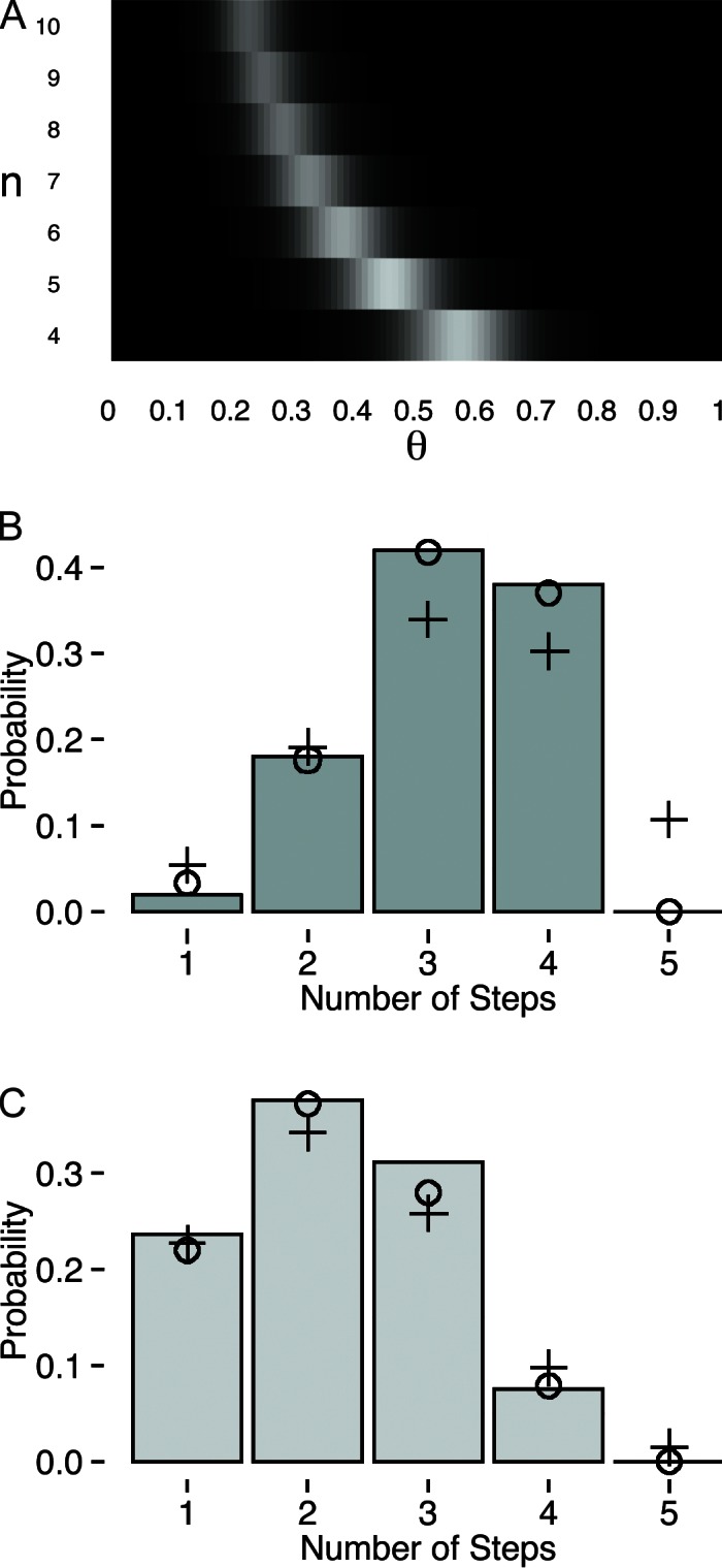
Ill-posed inference. (A) Joint posterior distribution of n and θ, given simulated data, y_N. Areas of lighter color reflect areas of higher posterior probability. Note that n can grow quite large and a compensation in θ results in high posterior probability. There does not generally exist a unique combination of n and θ that could produce some particular observations: this inference problem is ill posed. (B) Data drawn from a binomial distribution with n = 4 and θ = 0.8. (C) Data drawn from a binomial distribution with n = 4 and θ = 0.5. In B and C, circles (o) represent the best fit to a binomial distribution with n = 4, and crosses (+) represent the best fit to a binomial distribution with n = 5. In C, the best fits to the data for n = 4 and n = 5 are equally good because such fits are not unique.

To demonstrate how this ill-posed inference impairs our ability to learn n from data, Fig. 3 (B and C) shows simulated data meant to mimic the range seen in Fig. 1 (A and B) by drawing from a binomial distribution with n = 4 and θ equal to 0.8 (Fig. 3 B) and 0.5 (Fig. 3 C). In each case, we are tempted to conclude the true n is four, but can we make this assertion with equal vigor in both instances? An obvious approach is fitting binomial distributions to the data and assessing the quality of fit. The circles in Fig. 3 represent the best fit to a binomial distribution with n = 4, and it is clear that these fit the data well in both cases and that we are able to accurately estimate the optimal value of θ. However, to be confident about the assertion that n = 4, we must ask whether these fits are unique. The crosses in Fig. 3 show the best fit to a binomial distribution with n = 5. In Fig. 3 B, it is immediately obvious that even the best fit is a poor match to the data: the n = 5 binomial distribution underestimates the number of observed three and four bleaching steps and also predicts that roughly 10% of the data should have reflected five bleaching steps, whereas no five bleaching steps are observed. In this case, it is very obvious that n = 4. In Fig. 3 C, we cannot be so certain. Although the n = 4 binomial distribution certainly provides a good fit to the data, the n = 5 model also fits the data quite well for all observed bleaching steps. Furthermore, the n = 5 fit predicts that only 1% of the data should reflect five bleaching steps, and thus we might not have seen any simply because of the finite sample size. In this case, fits to the data are not unique and n and θ can compensate to produce identically good fits. This stems directly from the fact that this inference problem is ill posed, as depicted in the joint posterior distribution (Fig. 3 A). However, note that the possibility of this underestimation of n depends very strongly on the value of θ and qualitatively we can be more confident in the data in Fig. 3 B than Fig. 3 C. The methods proposed in the next section quantify this confidence.

Parameter confidence

Returning to example data, such as that in Fig. 3 (B or C), suppose we have observed some maximum number of bleaching steps, $\hat{k},$ and are tempted to conclude that n = $\hat{k}$ but want to consider the irksome possibility that n > $\hat{k},$ although we did not observe any evidence of it. We would like to make a statement to the effect of: Given N observations less than or equal to $\hat{k},$ we can conclude with confidence α that the true n is less than $\hat{k}$ + 1. The strategy proposed here is similar, in spirit, to classical hypothesis testing, where the null hypothesis is that n > $\hat{k}$ and 1 − α quantifies the probability of observing $\hat{k}$ under the null hypothesis.

As the null hypothesis, assume that n = $\hat{k}$ + 1, but we simply did not observe any y_i = $\hat{k}$ + 1 because of the finite sample size. For simplicity, assume (unrealistically) that we have an exact point estimate of θ for n = $\hat{k}$ + 1 denoted $\hat{\theta }$ (this assumption will be relaxed later). Then the probability of observing an event of size $\hat{k}$ + 1 is

$$\begin{array}{l}p(y_i=(\hat{k}+1\left)\right|\hat{k}+1,\hat{\theta })=\\ \frac{(\hat{k}+1)!}{\left(\right(\hat{k}+1)-(\hat{k}+1\left)\right)!(\hat{k}+1)!}{\hat{\theta }}^{\hat{k}+1}{(1-\hat{\theta })}^{\left(\right(\hat{k}+1)-(\hat{k}+1\left)\right)}\\ =\frac{(\hat{k}+1)!}{(\hat{k}+1)!}{\hat{\theta }}^{\hat{k}+1}{(1-\hat{\theta })}^0\\ ={\hat{\theta }}^{\hat{k}+1}.\end{array}$$

We then need to calculate the probability of not seeing this event, given that we have N observations. To do this, we consider the sampling distribution of events y_i = $\hat{k}$ + 1 under the null hypothesis, Bn($\hat{k}$ + 1,$\hat{\theta }$). This results in another binomial distribution, Bn(N,${\hat{\theta }}^{\hat{k}+1}$), where there are N chances of observing the event and the probability of the event is ${\hat{\theta }}^{\hat{k}+1}.$ Then the probability of $\hat{k}$ being the highest observed y_i is p(0|N,${\hat{\theta }}^{\hat{k}+1}$) and our estimate of confidence, α, is 1 − p(0|N,${\hat{\theta }}^{\hat{k}+1}$):

$$\begin{array}{l}\alpha =1-p\left(0\right|N,{\hat{\theta }}^{\hat{k}+1})\\ =1-\frac{N!}{(N-0)!0!}{\left({\hat{\theta }}^{\hat{k}+1}\right)}^0{(1-({\hat{\theta }}^{\hat{k}+1}\left)\right)}^N\\ =1-{(1-{\hat{\theta }}^{\hat{k}+1})}^N.\end{array}$$ (4)

As an approximate guide for experimental design, we can systematically explore the space of θ to understand how probable this underestimation actually is. Fig. 4 A plots α (confidence) for a region of θ and N and for a fixed value of $\hat{k}$ = 4. Again, smaller values of α mean that there is a higher probability of not observing the true tails of distribution under the null hypothesis. For smaller values of α, we cannot be confident that a dataset with a similar θ and N was not drawn from a binomial distribution that was larger than indicated by the data. For visual ease, the color map in Fig. 4 A focuses on several contours of α, and the colors threshold all α values to where they lie within these regimes. From this systematic exploration, some useful insights emerge. As we might have guessed, for large θ, the probability of underestimating the true n is trivially small, even for small datasets. However, for θ in the range of only 0.5, which has been seen multiple times in the literature (Coste et al., 2012; McGuire et al., 2012), this possibility is not so rare. This same information is presented in Table 1 in a more accessible form. For concreteness, Fig. 4 B shows α (confidence) as a function of sample size for two values of θ. For high θ, we can have high confidence in a conclusion even for a dataset of size 25. Conversely, if θ is 0.5, then a dataset of the same size would lead to the wrong conclusion with probability approximately 1/2. Returning to the data from Fig. 1, we can now (approximately) assess the strength of each of these data sources. We can be very confident in these data sources as 1 − α < 10⁶ in both instances. Fortunately, these two examples from the literature both provide reliable evidence that the CNG channel is a tetramer, although without using such methods, we would have been unable to quantify this confidence.

Figure 4.

Estimated parameter confidence. (A) Estimated α for various θ and sample sizes. The value of α is represented by the color map. For simplicity, contours of α are shown, and the color of each region indicates areas where α lies between these contours. (B) α as a function of sample size for two values of θ.

Table 1.

Approximate guide for experimental design

θ	n
	2	3	4	5	6	7	8
0.85	5	7	8	10	12	15	18
0.8	7	9	12	16	20	26	32
0.75	9	13	17	24	33	44	60
0.7	11	17	26	37	54	78	112
0.65	15	24	38	59	92	143	221
0.6	19	34	57	97	163	272	455
0.55	26	48	90	165	301	548	998
0.5	35	72	146	293	588	1,177	2,356
0.45	49	110	248	553	1,231	2,737	6,048

This table enumerates how many observations (N) would be required to achieve a confidence in excess of 0.99 for various values of θ and n.

It is also important to establish that our estimate of confidence with respect to the hypothesis n = $\hat{k}$ + 1 is a lower bound on all conceivable hypotheses n > $\hat{k}$ + 1. For simplicity, we will first consider the potential null hypothesis n = $\hat{k}$ + 2. Again, we are assuming that we have an optimal estimate $\hat{\theta },$ but now with respect to the model Bn($\hat{k}$ + 2,$\hat{\theta }$). As above, the probability of observing an event y_i = $\hat{k}$ + 2 is ${\hat{\theta }}^{\hat{k}+2}.$ Given that we have N observations, the probability of observing zero events of size y_i = $\hat{k}$ + 2 is

$$p\left(0\right|N,{\hat{\theta }}^{\hat{k}+1})={(1-{\hat{\theta }}^{\hat{k}+2})}^N.$$ (5)

The probability of observing an event of size y_i = $\hat{k}$ + 1 is

$$\begin{array}{l}p(\hat{k}+1|\hat{k}+2,\hat{\theta })\\ =\frac{(\hat{k}+2)!}{\left(\right(\hat{k}+2)-(\hat{k}+1\left)\right)!(\hat{k}+2)!}{\hat{\theta }}^{\hat{k}+1}{(1-\hat{\theta })}^{(\hat{k}+2)-(\hat{k}+1)}\\ =(\hat{k}+2){\hat{\theta }}^{\hat{k}+1}(1-\hat{\theta }).\end{array}$$

The probability of observing exactly zero of these events, given a total of N observations is

$$p\left(0\right|N,(\hat{k}+2){\hat{\theta }}^{\hat{k}+2}(1-\hat{\theta }))={(1-(\hat{k}+2\left){\hat{\theta }}^{\hat{k}+1}\right(1-\hat{\theta }\left)\right)}^N.$$ (6)

The probability of seeing no observations of size $\hat{k}$ + 1 or $\hat{k}$ + 2 is just the product of Eqs. 5 and 6. Therefore, our confidence that true n is not $\hat{k}$ + 2 goes as

$$\alpha =1-{(1-{\hat{\theta }}^{\hat{k}+2})}^N{(1-(\hat{k}+2\left){\hat{\theta }}^{\hat{k}+1}\right(1-\hat{\theta }\left)\right)}^N.$$ (7)

Generally, the estimate $\hat{\theta }$ used in Eq. 5 will be less than that of Eq. 4 (see Fig. 3 A). However, the confidence estimate in Eq. 7 involves multiplication with an additional term than Eq. 4. Therefore, the confidence estimated when considering the hypothesis n = $\hat{k}$ + 2 will always be higher than that for the hypothesis n = $\hat{k}$ + 1. This is visualized in Fig. 5 where confidence is plotted as a function of sample size for the null hypothesis n = $\hat{k}$ + 1 as well as for the null hypothesis n = $\hat{k}$ + 2. Clearly, the estimate of confidence with respect to $\hat{k}$ + 1 is the most conservative estimate. It is easy to see that this relationship will persist for all n > $\hat{k}$ + 1. Because of this, we only need to calculate confidence with respect to $\hat{k}$ + 1, as this provides a lower bound on confidence with respect to all possible n > $\hat{k}.$

Figure 5.

Comparison of parameter confidence when considering multiple models. The black curve is a plot of confidence versus sample size for the null hypothesis n = $\hat{k}$ + 1. The gray curve is the parameter confidence for the null hypothesis n = $\hat{k}$ + 2. It is clear that only the hypothesis n = $\hat{k}$ + 1 needs to be considered and will result in an estimate of confidence that is a lower bound on all possible hypotheses.

The previous discussion provides a notion of confidence only if we know the value of θ exactly. As this is never the case (Fig. 2), we need to generalize Eq. 4 to include our uncertainty in the value of θ. This uncertainty is quantified by the conditional posterior distribution, p(θ|y_N,$\hat{k}$ + 1), with respect to the null hypothesis n = $\hat{k}$ + 1. Our estimate of confidence should consider all possible values of θ, weighted by their posterior probability. In particular,

$$\begin{array}{l}\alpha =1-{\displaystyle \underset{0}{\overset{1}{\int }}p\left(0\right|N,{\theta }^{\hat{k}+1}\left)p\right(\theta |y_N,\hat{k}+1)d\theta }\\ =1-{\displaystyle \underset{0}{\overset{1}{\int }}p\left(0\right|N,{\theta }^{\hat{k}+1}\left)Be\right(A,B)d\theta }\\ =1-\frac{1}{\beta (A,B)}{\displaystyle \underset{0}{\overset{1}{\int }}{(1-{\theta }^{\hat{k}+1})}^N{\theta }^A{(1-\theta )}^{B}d\theta ,}\end{array}$$ (8)

where A and B are calculated from observed distribution as in Eq. 2. In the absence of a simple form of the integral in Eq. 8, we turn to Monte Carlo integration. Calculation of α entails integrating a function over a probability distribution. In particular, integration is over the conditional posterior of θ, i.e.,

$${\displaystyle \underset{0}{\overset{1}{\int }}f\left(\theta \right)p\left(\theta \right|y_N,\hat{k}+1)}d\theta ,$$

where f(θ) is the probability of observing zero events of size $\hat{k}$ + 1 under the null hypothesis. If we can draw independent and identically distributed (iid) samples from a probability distribution, then a finite number of such samples can be used to approximate the integration. For example, if we draw S samples $\tilde{\theta }$ from the distribution p(θ), then

$${\displaystyle \int f\left(\theta \right)p\left(\theta \right)d\theta \approx \frac{1}{S}{\displaystyle \sum _{i=1}^{S}f\left({\tilde{\theta }}_i\right).}}$$

Fortunately, the form of the conditional posterior of θ is simple (Eq. 2), so generating iid samples, $\tilde{\theta },$ can be achieved by drawing Beta random variables: $\tilde{\theta }$ ∼ Be(A,B). Then α can be estimated as

$$\begin{array}{l}\alpha \approx 1-\frac{1}{S}{\displaystyle \sum _{i=1}^{S}p\left(0\right|N,{\left({\tilde{\theta }}_i\right)}^{\hat{k}+1})}\\ =1-\frac{1}{S}{\displaystyle \sum _{i=1}^S{(1-{\left({\tilde{\theta }}_i\right)}^{\hat{k}+1})}^N.}\end{array}$$ (9)

In this way, a proper estimate of confidence can be calculated that takes into account the total uncertainty in all of the model parameters. The Monte Carlo integral in Eq. 9 converges quickly as is shown in Fig. 6 A, which is a plot of the estimate of α (for some simulated dataset) as a function of the number of samples, $\tilde{\theta }.$ In Fig. 6 B is a comparison of the estimate of confidence as calculated using the two methods developed so far. The smooth curve is a plot of confidence as a function of sample size for a point estimate of θ (${\alpha }_{\hat{\theta }}$). The circles are the corresponding estimate of confidence using the Bayesian model (α_B), which takes into account the full uncertainty in θ. Generally, the simplified estimation of confidence (${\alpha }_{\hat{\theta }}$) overestimates confidence because of the assumption that θ is known with certainty. Indeed, the estimated confidence when considering the full parameter uncertainty is consistently less than with the simplified approach, and thus this method affords a more realistic and conservative estimate of parameter confidence. Finally, note that as N increases, so too will A and B (of Eq. 2). The result is that the conditional posterior of θ becomes narrowed and more probability mass is located closer to the optimal estimate, $\hat{\theta }$ (see Fig. 2). In the limit of large N, the posterior of θ shrinks to a point estimate, and confidence calculated via Eq. 8 converges exactly to Eq. 4 (see also Fig. 6 B). Thus, the Bayesian method presented here is a generalized approach that collapses to the more simplified estimate in the limit of large sample sizes.

Figure 6.

Estimation of parameter confidence using Monte Carlo integration. (A) The estimate of confidence from Eq. 9 as a function of the number of posterior samples, $\tilde{\theta },$ used for Monte Carlo integration. This estimate converges quickly. (B) Confidence as a function of sample size estimated using a point estimate of θ (${\alpha }_{\hat{\theta }}$) and the Bayesian estimate (α_B). It is clear that ${\alpha }_{\hat{\theta }}$ overestimates parameter confidence and that the true uncertainty in θ must be taken into account for an accurate estimate of confidence.

I now address a related problem when interpreting such data, which is discussed only briefly as the basic method was proposed previously in Groulx et al. (2011). Consider that an imperfect data collection algorithm induces artifactual observations into the distribution. In particular, suppose that the largest number of observed bleaching steps, $\hat{k},$ occurs with an anomalously low prevalence and we are tempted to conclude that all y_i = $\hat{k}$ are artifacts and the true n is $\hat{k}$ − 1. Given that we have observed K events of size $\hat{k},$ we simply need to consider the sampling distribution of events of size $\hat{k}$ under the hypothesis Bn($\hat{k},$θ) and calculate the rarity of K in this sampling distribution. As before, this sampling distribution is binomial, Bn(N,${\theta }^{\hat{k}+1}$), and we simply calculate p(K|N,${\theta }^{\hat{k}+1}$). Previous authors estimated this sampling distribution using the Poisson approximation to the binomial distribution and using a fixed estimate of θ (see supplemental material in Groulx et al. [2011]). I generalize this by considering the full uncertainty in the estimate of θ. The probability of observing K or fewer events of size $\hat{k}$ under the null model Bn($\hat{k},$θ) will be denoted γ. If we integrate over the uncertainty in θ, then γ is calculated as

$$\begin{array}{l}\gamma ={\displaystyle \underset{0}{\overset{1}{\int }}\left[{\displaystyle \sum _{j=1}^{K}p\left(j\right|N,{\theta }^{\hat{k}}\left)p\right(\theta |y_N,\hat{k})}\right]d\theta }\\ \approx \frac{1}{S}{\displaystyle \sum _{i=1}^S\left[{\displaystyle \sum _{j=1}^{K}p\left(j\right|N,{\left({\tilde{\theta }}_i\right)}^{\hat{k}})}\right]}\\ =\frac{1}{S}{\displaystyle \sum _{i=1}^S\left[{\displaystyle \sum _{j=1}^K\frac{N!}{(N-j)!j!}{\left({\left({\tilde{\theta }}_i\right)}^{\hat{k}}\right)}^j{(1-{\left({\tilde{\theta }}_i\right)}^{\hat{k}})}^{N-j}}\right]}.\end{array}$$ (10)

Here, we again draw samples, $\tilde{\theta },$ from the posterior of θ to use for Monte Carlo integration. This integration is approximated by the sum over i in the above equation. The rest of Eq. 10 is the sampling distribution of observations of size $\hat{k},$ and we sum up to K to calculate the probability of seeing K or fewer observations. If γ is very small, it means that our observation of K instances of size $\hat{k}$ is quite rare under the model Bn($\hat{k},$θ) and that we might exclude all observations of size $\hat{k}$ as artifacts and accept the hypothesis n = $\hat{k}$ − 1. I have provided code for the implementation of this analysis, as well as the calculation of α (Eqs. 8 and 4; see Supplemental material.)

A potential complication that has been ignored in this work is the possibility of multiple complexes within the same observation volume. This could occur if the density of complexes is sufficiently high or if complexes have a tendency to cluster together. In this instance, the observed distribution of bleaching events would be drawn from a heterogenous population of species, some of which contain n subunits and others which contain some multiple of n subunits. In fact, this complication seems to be fairly common in the literature, and the interpretation of such artifactual data needs to be formally addressed. In previous work, the strategy of fitting sums of binomial distributions proved successful at overcoming this complication (McGuire et al., 2012). This strategy would be useful only to the extent that the uniqueness of fits could be established. In principle, the methods presented in this paper could be generalized to a model of heterogeneous populations of binomially distributions observations. Such a model would necessarily have more parameters, which would exacerbate the problem of ill-posed inference. However, I believe that methods of confidence estimation should be applicable to a more generalized model. Future work remains to be done in this area.

Conclusions

Single molecule photobleaching is a pervasive tool for determining protein association that relies on attaching fluorescent probes to molecules of interest and counting distinct photobleaching events. Because there is a nonzero probability of not observing a particular fluorophore, the resulting distribution of photobleaching steps will be binomial. Although it seems a straightforward task to interpret such data and deduce stoichiometry, it was shown that this inference is ill posed. This means that many possible combinations of n and θ can produce very similar observations. Because there is not generally a unique and optimal estimate of the relevant parameters for a given dataset, extracting the stoichiometry can be error prone without careful analysis. A general inference model was developed for this type of data that takes into account the full uncertainty in all model parameters. Using this framework, methods were developed for hypothesis testing and calculating parameter confidence that allow for a rigorous interpretation of such data. This work provides a rigorous analytical basis for the interpretation of single molecule photobleaching experiments.

References

- Arumugam S.R., Lee T.H., Benkovic S.J. 2009. Investigation of stoichiometry of T4 bacteriophage helicase loader protein (gp59). J. Biol. Chem. 284:29283–29289 10.1074/jbc.M109.029926 [DOI] [PMC free article] [PubMed] [Google Scholar]
- Coste B., Xiao B., Santos J.S., Syeda R., Grandl J., Spencer K.S., Kim S.E., Schmidt M., Mathur J., Dubin A.E., et al. 2012. Piezo proteins are pore-forming subunits of mechanically activated channels. Nature. 483:176–181 10.1038/nature10812 [DOI] [PMC free article] [PubMed] [Google Scholar]
- Demuro A., Penna A., Safrina O., Yeromin A.V., Amcheslavsky A., Cahalan M.D., Parker I. 2011. Subunit stoichiometry of human Orai1 and Orai3 channels in closed and open states. Proc. Natl. Acad. Sci. USA. 108:17832–17837 10.1073/pnas.1114814108 [DOI] [PMC free article] [PubMed] [Google Scholar]
- Ding H., Wong P.T., Lee E.L., Gafni A., Steel D.G. 2009. Determination of the oligomer size of amyloidogenic protein β-amyloid(1-40) by single-molecule spectroscopy. Biophys. J. 97:912–921 10.1016/j.bpj.2009.05.035 [DOI] [PMC free article] [PubMed] [Google Scholar]
- Groulx N., McGuire H., Laprade R., Schwartz J.L., Blunck R. 2011. Single molecule fluorescence study of the Bacillus thuringiensis toxin Cry1Aa reveals tetramerization. J. Biol. Chem. 286:42274–42282 10.1074/jbc.M111.296103 [DOI] [PMC free article] [PubMed] [Google Scholar]
- Ji W., Xu P., Li Z., Lu J., Liu L., Zhan Y., Chen Y., Hille B., Xu T., Chen L. 2008. Functional stoichiometry of the unitary calcium-release-activated calcium channel. Proc. Natl. Acad. Sci. USA. 105:13668–13673 10.1073/pnas.0806499105 [DOI] [PMC free article] [PubMed] [Google Scholar]
- McGuire H., Aurousseau M.R., Bowie D., Blunck R. 2012. Automating single subunit counting of membrane proteins in mammalian cells. J. Biol. Chem. 287:35912–35921 10.1074/jbc.M112.402057 [DOI] [PMC free article] [PubMed] [Google Scholar]
- Nakajo K., Ulbrich M.H., Kubo Y., Isacoff E.Y. 2010. Stoichiometry of the KCNQ1 - KCNE1 ion channel complex. Proc. Natl. Acad. Sci. USA. 107:18862–18867 10.1073/pnas.1010354107 [DOI] [PMC free article] [PubMed] [Google Scholar]
- Reiner A., Arant R.J., Isacoff E.Y. 2012. Assembly stoichiometry of the GluK2/GluK5 kainate receptor complex. Cell Rep. 1:234–240 10.1016/j.celrep.2012.01.003 [DOI] [PMC free article] [PubMed] [Google Scholar]
- Ulbrich M.H., Isacoff E.Y. 2007. Subunit counting in membrane-bound proteins. Nat. Methods. 4:319–321 [DOI] [PMC free article] [PubMed] [Google Scholar]
- Ulbrich M.H., Isacoff E.Y. 2008. Rules of engagement for NMDA receptor subunits. Proc. Natl. Acad. Sci. USA. 105:14163–14168 10.1073/pnas.0802075105 [DOI] [PMC free article] [PubMed] [Google Scholar]
- Yu Y., Ulbrich M.H., Li M.H., Dobbins S., Zhang W.K., Tong L., Isacoff E.Y., Yang J. 2012. Molecular mechanism of the assembly of an acid-sensing receptor ion channel complex. Nat. Commun. 3:1252 10.1038/ncomms2257 [DOI] [PMC free article] [PubMed] [Google Scholar]
Associated Data
This section collects any data citations, data availability statements, or supplementary materials included in this article.