Accurate detection of differential RNA processing

Abstract

Deep transcriptome sequencing (RNA-Seq) has become a vital tool for studying the state of cells in the context of varying environments, genotypes and other factors. RNA-Seq profiling data enable identification of novel isoforms, quantification of known isoforms and detection of changes in transcriptional or RNA-processing activity. Existing approaches to detect differential isoform abundance between samples either require a complete isoform annotation or fall short in providing statistically robust and calibrated significance estimates. Here, we propose a suite of statistical tests to address these open needs: a parametric test that uses known isoform annotations to detect changes in relative isoform abundance and a non-parametric test that detects differential read coverages and can be applied when isoform annotations are not available. Both methods account for the discrete nature of read counts and the inherent biological variability. We demonstrate that these tests compare favorably to previous methods, both in terms of accuracy and statistical calibrations. We use these techniques to analyze RNA-Seq libraries from Arabidopsis thaliana and Drosophila melanogaster. The identified differential RNA processing events were consistent with RT–qPCR measurements and previous studies. The proposed toolkit is available from http://bioweb.me/rdiff and enables in-depth analyses of transcriptomes, with or without available isoform annotation.

INTRODUCTION

Deep RNA sequencing has enabled profiling the transcriptional landscape of the cell at unprecedented resolution [e.g. (1,2)]. Technological advances have dramatically increased the read coverage and the dynamic range of RNA-Seq, facilitating a wide range of analyses to answer pertinent questions. One of the most fundamental analyses is comparative transcriptome analysis of samples that have been exposed to different environmental conditions or have variable genetic background. The development of computational tools to carry out such pairwise comparisons is a field of active research and the subject of this work.

For single isoform genes, the true mRNA isoform abundance is tightly coupled to the number of reads that map to exonic regions of the corresponding gene (2). A widely used model to explain the number of mapping reads as a function of the unknown abundance is the binomial model and its Poisson limit. Several early methods have directly used such idealized statistics to test for differential expression between samples from the raw read count information [e.g. (3,4)]. More recent extensions (5–8) generalize the basic Poisson model to a more flexible class of distributions, such as negative binomial (NB) models. In contrast to Poisson-based tests, these models account for so-called overdispersion, i.e. the empirical variability of counts because of biological or technical factors.

The large majority of genes of higher eukaryotes have multiple annotated isoforms that are the result of alternative usage of transcription starts, splice sites, RNA editing sites or polyadenylation sites. Defining gene expression in the case of multiple isoforms becomes conceptually difficult and testing for differential gene expression can easily be confounded by differential RNA processing events, such as alternative splicing. In particular, the number of observed RNA-Seq reads may significantly change, even if the total number of RNA molecules remains constant. This may occur, for instance, if a significant part of the RNA molecule is excised during splicing. An alternative is to test for differential expression of an isoform in multiple samples. However, if one of the samples is subject to a significant increase of transcriptional activity of a gene, under this test, all alternative isoforms would be detected as differentially expressed.

In this work, we are interested in an alternative formulation. We seek to identify significant differences in relative isoform expression. Importantly, these relative abundances are insensitive to overall gene expression changes, but they reflect changes because of differential RNA processing. See Figure 1 for an illustration.

Figure 1.

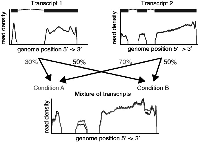
On the top, two transcripts are shown together with the read density one would observe if they were present isolated from each other. On the bottom, the read densities for two mixtures of the transcripts are shown. The mixture for the conditions A (light gray) and B (dark gray) is different, which is reflected by the difference of the read densities.

Recently, several algorithms for inferring the abundance of a given set of isoforms based on the observed read coverages have been proposed (9–13). These approaches solve the problem of deconvolving the observed read coverage and implicitly or explicitly assigning reads to individual isoforms. The difficulty of assigning reads to isoforms comes from the fact that these are often near-identical and a read from an overlapping region cannot be assigned to a specific isoform without additional information. Perhaps the most advanced approaches are those carrying out full Bayesian inference, such as MISO (13) or BitSeq (14), propagating and accounting for uncertainty and covariation of expression estimates from multiple overlapping isoforms. In general, for all of these methods, the estimated abundances typically correlate well but far from perfectly with other experimental data, such as qPCR and NanoString measurements of RNA isoform abundances, in particular when many isoforms are present (A. Mortazavi, personal communication).

A natural and appealing strategy is to combine methods to estimate isoform abundance for different RNA-Seq experiments with a statistical test for differential expression of isoforms. However, the solution to the quantification problem may not be unique [see, for instance, discussions in Lacroix et al. and Hiller et al. (15,16)]. This problem can be partially alleviated by estimating confidence intervals for the abundance estimates, either by evaluating the Fisher information matrix (9) or by conducting full Bayesian inference (13,14), but the estimation of this correlation structure is technically challenging and depends on a number of assumptions that may not always be satisfied in practical settings. Most sophisticated approaches, such as characterizing the non-unique solutions using Markov Chain Monte Carlo methods (13,14), circumvent some of these weaknesses, at the price of considerable computational cost. Further, if one is only interested in which genes or isoforms are differentially expressed, first quantifying and then testing for differential expression might be an unnecessary detour, solving a harder task than actually required.

In this work, we seek alternative strategies for detecting differential abundances of RNA isoforms in pairs of biological samples. We focus on the case where the sum of the abundances of all isoforms either remains constant or as such is irrelevant, and the abundances of the isoforms between two conditions vary (Figure 1). This setting is particularly interesting for analyzing RNA-Seq experiments with the aim to gain a deeper understanding of RNA modifying processes (such as alternative splicing or polyadenylation).

The devised approaches are simple and implemented as a single step, avoiding the need to quantify isoform abundances first. Importantly, they operate on the level of isoforms and are not restricted to differences on the level of the overall expression of a given gene. First, we propose a test called rDiff.parametric, extending established Poisson and NB-based tests for detecting differential expression of genes to testing for differential isoform abundance. The idea is to identify genomic regions based on the given isoform annotation that are not shared among all isoforms and detect differences in the read coverage in these informative regions (compare regions marked in light green in Figure 2a). We show how this principle can be used to build efficient statistical tests to identify regions with alternative isoform expression. Second, we propose rDiff.nonparametric, an approach that can detect differential isoform abundance without depending on any knowledge of the underlying isoform structure. To avoid the need to quantify within known regions, the approach directly assesses differences of the read mapping distribution at a predefined genomic locus. This test is especially useful for the large number of newly sequenced genomes where the gene structure is often only determined by homology to already annotated species. The parametric variant, rDiff.parametric, shares many ideas and concepts with recent work, such as DEXSeq (17). However, DEXSeq is aimed at modeling the exon-specific abundance rather than transcripts and does not extend to settings without transcript annotation. Conceptually, the non-parametric testing approach has previously been described in Stegle et al. (18), and related ideas have later been proposed in (19). There the authors followed a similar idea but concentrated on counts on splice junctions in a constructed splicing graph. Importantly, their approach does not consider a variance model as used in rDiff and DEXSeq (17) [as well as in DESeq (7) and edgeR (20)].

Figure 2.

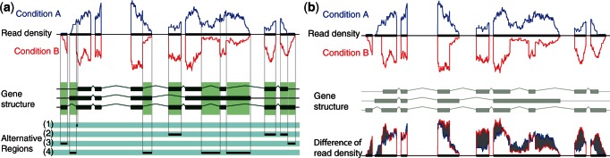
(a) The alternative regions used by rDiff.parametric. Alternative regions are defined as regions in the genome that are not contained in all transcripts of a gene but at least one, according to the gene structure. In a second step, all regions are merged, which are in the same subgroups of transcripts, to obtain the so-called alternative regions. (b) Test statistic used by rDiff.nonparametric. Shown are the two read densities in the two conditions A and B and their difference in gray and the underlying gene structure in light green.

We perform a detailed simulation study to comprehensively compare rDiff.nonparametric and rDiff.parametric with existing methodology and to elucidate the strengths and limitations of the algorithms. Moreover, we illustrate the algorithms’ practical use in a realistic setting of three RNA-Seq libraries from Arabidopsis thaliana and four libraries from Drosophila melanogaster. We find that the detection of alternative events is reliable and in concordance with results from RT–qPCR (reverse transcription–quantitative polymerase chain reaction), even when the gene structure is not used.

MATERIALS AND METHODS

We start by introducing the statistical read model and present a practical scheme to estimate biological variability on splicing data. Building on this description, we introduce a first statistical test that exploits complete information on the gene annotation. Finally, we provide a non-parametric variant that can be used when the isoform annotation is incomplete or missing.

Read statistics

When doing inference from read counts it is important to account for the fact that reads are generated by a random sequencing procedure. Thus, read counts should not be treated as fixed values but instead as draws from a suitable distribution to capture random fluctuation.

Previous work on differential testing of whole-gene expression established the duality of types of noise variation that are dominant in specific regimes (6–8,20). First, read data are subject to shot noise because of the nature of sequencing data from random sampling. This noise is dominant for low read counts. Second, overdispersion because of biological variation increases the expected noise level as empirically observed between biological replicates. The first type of variance is well described by a linear relationship between mean and variances, whereas the second type is characterized by a quadratic component. Contrary to the shot noise, the effect of overdispersion is strongest for high counts. The variance caused by different barcodes or the use of different mappers for the samples also has a quadratic component and can for simplicity be considered as part of the biological variance. Here, we follow largely the approaches proposed previously (7,20) and build on NB distributions to model the read counts. A major difference to these approaches is that we do not model the counts for gene expression but for smaller regions that are indicative of a change in relative isoform abundance. Throughout, we assume that the variance of the distribution for a given read count is a function of the expression abundance. This empirical variance function estimates the variance to be expected for different expression levels. For a detailed discussion of our statistical model we refer to Supplemental Section S1.

Variance estimation

The estimation of biological variance is an integral building block to differentiate true differences from fluctuations caused by biological or technical variation. Let in the following G be the set of genes and R be a biological sample that consists of a set of replicates . For all genes and replicates , we assume to have an estimate of the gene expression and read counts for each region , where J_g is the set of regions in gene g. We estimated the biological variance by using replicate data, to get the means and variances of tuples of normalized read counts in the replicates. To detect changes in the relative transcript abundances and not changes in absolute abundance, we computed a normalizing constant

The normalization makes counts comparable across the replicates when having variability in gene expression (which may have different total numbers of reads).

We then computed normalized counts . For each region in gene g, we then estimated the mean of the normalized counts

as well as their empirical variance:

Finally, we performed a local regression on the set of points [similar to the procedure proposed previously (7)] to obtain a functional mapping f_R between the empirical mean to the expected variance. This was done using the Locfit (21) package.

Working without replicates.

If replicate data are not available, conservative estimates of the variance function can be obtained from between-sample fits. Following (7), one can consider the two samples A and B as replicates to fit the variance function. If there are no differential sites, this approximation is fully legitimate, whereas in the presence of true differences, one can expect an overestimation of the variance fits, leading to a conservative approximation. Alternatively, one can use an estimated variance function from a similar sample as the ones under investigation.

Statistical testing with known gene structure

Defining alternative regions

Given a known and complete gene annotation, differential isoform abundance can be detected by differential comparison of a set of restricted exonic regions, denoted alternative regions in the following (Figure 2a). These regions are defined as isoform-specific loci, i.e. those positions where reads map that can only stem from a non-empty strict subset of all isoforms. Relative changes of the abundance between isoforms can in principle be only observed at those positions; hence, the remainder of exonic loci can be left aside.

To avoid explicitly solving the deconvolution problem of multiple overlapping isoforms, we grouped the alternative regions into areas that are absent or present in the same isoforms. The resulting grouped regions are the regions on which we tested for differences in relative abundance between isoform with respect to the total gene expression.

Testing for changes

Statistical testing is carried out in each alternative region of a gene g. As the testing is performed for one gene at a time, we omit the index g for simplicity of notation. Our null hypothesis H₀ is that there is no differential expression in a particular region. Formally, this corresponds to the read in intensity relative to the gene expression being the same in a region j for samples and , where u is the number of replicates in sample A and v the number of replicates in sample B. Under this hypothesis, the number of counts we expect to observe in sample A in region j can be calculated by the normalized mean expression q_j for both samples, i.e. by averaging the normalized reads in all samples:

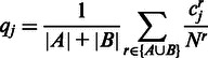(1)

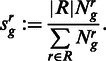
where r runs over the replicates from either sample A and B, N^r is the gene expression in replicate r and is the number of reads mapping to region j in replicate r. Using the normalized expression, we then calculated the average number of counts we expect to see under the null hypothesis as 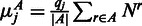. The calculations for were analogous. The distribution under the null hypothesis was computed as follows. Let 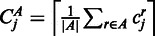and be the rounded up average number of observed reads in a region j. We assumed that the observed counts are drawn from an NB distribution 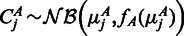and 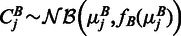, where f_A is the variance function estimated for sample A and analogous for f_B. 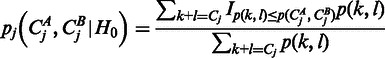For brevity denote by , the joint probability of observing k reads in sample A and l reads in sample B. Denote furthermore the total read counts in region j as . Then the P-value p_j of the observed counts and under the null hypothesis H₀ is given by:

(2)

where I_T is an indicator function that is 1 if T is true and 0 otherwise. Finally, we combined the P-values across regions into a genewise P-value of relative transcript abundance variability using a conservative Bonferroni correction (22):

(3)

We refer to this method as rDiff.parametric. Alternatively, the information as to which specific testing region is differentially expressed can be used directly, which is similar as the approach taken previously (17).

Testing with unknown gene structure

In many cases, the gene annotation is not available; hence, alternative regions cannot be defined a priori. We propose an alternative strategy to test changes in the read density at the whole-genomic locus. Our approach builds on the non-parametric Maximum Mean Discrepancy (MMD) test (23,24).

This flexible two-sample test for high-dimensional vectors is well suited for our setting, as it poses few assumptions on the distribution of the reads. The basic idea of this test applied to our setting is to represent the reads A_g and B_g that map to gene g in samples A and B in the space , where l_g is the length of g. This is done by representing each read i in sample r as a vector of length l_g. The entry of at the jth dimension is 1 if the read covers the jth position of the gene and 0 otherwise. In this space, the mean for the sample r is given by:

where K^r is the number of reads in the sample r. The difference 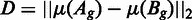between the two read densities A_g and B_g is then computed and used as the test statistic (see Figure 3 for an illustration). To determine the significance of the distance D, this value is compared with an empirical null distribution, estimated from T differences between two random samples from the joint read distribution .

Figure 3.

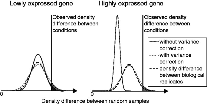
Illustration of variance of the read density difference (see gray area in Figure 2b) between random samples from the null distribution. The distribution difference between two biological samples is shown as a dashed black curve, the one between two random samples when not correcting for biological variance in dark gray dashed and when correcting for biological variance in light gray dashed. The resulting P-value for rDiff.nonparametric corresponds to the gray area of surface, which is the fraction of random samples that have a bigger difference than the difference observed between the two conditions. For highly expressed genes, when not correcting for biological variance, the density difference between random samples converges to zero, thus leading to an unrealistically small P-value.

The basic MMD strategy described earlier in the text was extended in two different ways: (i) we accounted for biological variance by sampling such that the variance of the random samples was in concordance with the empirically fitted biological variance model.

This extension of the original bootstrapping procedure leads to an appropriate variance of the null distribution as illustrated in Figure 3, thereby avoiding an oversensitivity on highly expressed genes. The P-value was estimated by the number of times the observed difference D is larger than D_t: . For a detailed description, see Supplementary Section S2.1. (ii) We increased the power by preferentially focusing on regions in the gene that could potentially reflect a differentially processing. We observed empirically that one can increase the power of the MMD test, when only considering genomic positions that have a lower than maximal read coverage in one of the samples. This observation can be explained by the fact that the regions with large relative coverage are unlikely to be differentially covered between samples (as this would require them to be not fully covered in at least one sample and thus cannot have a maximal coverage). Exploiting this characteristic, we perform several tests on the subsets of the positions where the coverage is below different thresholds. More specifically, we applied the MMD test on the 10% of the positions that have the lowest positive coverage to obtain a P-value p₁₀. Subsequently, we repeated the procedure for 20% and so forth until we had 10 P-values . These P-values were combined, Bonferroni corrected and reported as the result of rDiff.nonparametric.

Data sets used for evaluation

We considered a data set from A. thaliana to apply and compare the proposed methods.

For this study, A. thaliana Wt seedlings were grown in darkness and exposed to light for 0, 1 or 6 h. Furthermore, we used cry1cry2 seedlings (25,26) grown under the same conditions as the 0 h Wt seedlings.

The mRNA libraries were prepared using the Illumina mRNA-Seq 8-sample Prep kit. We sequenced 80 bp reads on the Illumina GAIIx platform using a single-end flow cell, resulting in ∼3.9 × 10⁷ reads per lane on average. In each library, a variable fraction between 86.3 and 87.4% of reads could be uniquely aligned to the genome using Palmapper (27), resulting in an average coverage of the transcriptome of ∼51-fold per lane. For ∼24% of the reads, the best alignment obtained was a spliced alignment, i.e. it spanned an exon–exon border. Full details on the experimental design and implementation can be found in Supplementary Section S5.

Simulation approach

In addition to empirical data, we also created two artificial data sets to have data sets with exact ground truth expression levels. We focused on the 5875 mRNA coding genes in the A. thaliana TAIR10 reference annotation that have at least two splice variants. Both artificial data sets consisted of samples for two different conditions with two simulated biological replicates each. To simulate a realistic extent of biological variance, we estimated the gene expression variance on experimental data described before. In a first simulated setting, we used the two samples grown with 0 h light exposition to estimate the biological variance and an additional sample from the seedlings 1 h to get realistic gene expressions for the simulated conditions. The true simulated isoform abundances were drawn from a uniform distribution, and the absolute gene expression abundance was drawn from the expressions measurements. For half of the genes, we simulated a differential relative isoform expression. Furthermore, we simulated a biological variance in both samples by drawing isoform abundances such that the resulting variance of the reads matched the estimated biological variance.

To assess the effect and relevance of biological variance, we repeated the same simulation procedure with increased biological variability. In this second simulated data set, we considered the variation between the samples at 0 h and 1 h to simulate the biological variance. Full details of the read simulation can be found in Supplementary Section S3.

False discovery rate estimation

As a measure of the genome wide significance of the findings, we used the false discovery rate (FDR). The FDR was calculated as described previously (28).

RESULTS

Evaluation on synthetic data

Benchmark data and alternative methods

For objective comparison of alternative methods, we considered two realistic simulated data sets (see ‘Materials and Methods’). We used the proposed models either explicitly using the gene annotation (rDiff.parametric) or not using the annotation (rDiff.nonparametric). For comparative purposes, we also considered two state-of-the-art methods that explicitly quantify transcript isoforms to test for differences, MISO (13) and cuffDiff (29). To assess the impact of modeling biological variance, we also applied the simplified variant of the parametric test, called rDiff. poisson, which is based on the Poisson distribution instead of the NB distribution. A detailed description of how the competing methods were applied is found in Supplementary Section S4.

Ranking of differentially expressed genes

First, we evaluated the ranking of differentially expressed genes produced by alternative methods. To quantify their respective performances, we used the receiver operating characteristics (ROC), depicting the true-positive rate (TPR) of predictions for different false-positive rates (FPR). For biological applications, the most confident predictions with a moderate FPR are most relevant; thus, we restrict the interval of considered FPR to at most 0.2. The ROC curves for each method evaluated on the synthetic data set are shown in Figure 4, and a tabular summary of the area under the ROC curve is given in Table 1. rDiff.parametric consistently outperformed cuffDiff and MISO with the differences being most striking for most confident calls, where rDiff.parametric achieved a substantially higher TPR. The Poisson-based parametric model (rDiff.poisson) was slightly, but consistently, outperformed by its NB counterpart. rDiff.nonparametric performed as well as MISO and cuffDiff, which is surprising, given the fact that our approach does not use the gene annotation and is conceptually much simpler. This finding highlights the applicability and practical use of the simple one-step methods, both in settings where the genome annotation is available but also if it is incomplete or missing.

Figure 4.

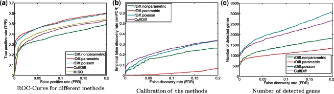
Comparison of rDiff with MISO and CuffDiff. (a) ROC curve for rDiff, MISO and CuffDiff. (b) Comparison of the empirical false discovery rate (empFDR) and the FDR based on P-values provided by the methods, for rDiff and CuffDiff. This was not possible for MISO, as it did not provide P-values. (c) Number of detected genes as a function of the FDR cut-off.

Table 1.

Area under the ROC curve in the interval (0, 0.2) (auROC20) for rDiff, cuffDiff and MISO

Method	auROC20 for small biol. variance	auROC20 for large biol. variance
rDiff.nonparametric	0.077	0.073
rDiff.parametric	0.101	0.093
rDiff.poisson	0.099	0.082
cuffDiff	0.085	0.055
MISO	0.089	0.061

The comparison is shown on the two artificial data sets with a small and large biological variance (see ‘Materials and Methods’ section).

To investigate the robustness of the different methods with respect to biological variability, we considered a second synthetic data set with larger biological variation (Supplementary Figure S2a). Although the previously observed trends still hold, the differences between the respective methods were more pronounced. The performance of MISO, rDiff.poisson (which does not model biological variance) and cuffDiff decreased dramatically, in particular for low FPR. rDiff.parametric and rDiff.nonparametric both consider biological variability for computing significance levels and perform best, in particular for the most confident cases. This emphasizes the relevance of modeling biological variability.

Calibration of test statistics

It is important that the tests deliver meaningful significance levels and false discovery estimates. Therefore, we tested the statistical calibration of the calling confidences provided by the different methods by comparing the estimated FDRs with the empirical FDRs (empFDR). The latter is known because we simulated the data. The empirical FDR was calculated as the fraction of false positives in the number of genes having P-values below a certain threshold. Figure 4b shows the calibration curves for all methods on the first synthetic data set. rDiff.parametric was the most conservative approach, and the empirical FDR was about three times smaller than the estimated FDR (at 0.2). rDiff.nonparametric was less conservative (empirical FDR ∼1.3 times smaller than estimated FDR) and overall achieved an acceptable level of calibration. cuffDiff and rDiff.Poisson, however, seemed to be overoptimistic by calling a large number of false positives for small FDRs: the most confident predictions were false. This behavior is likely caused by the lack of control for biological variance. MISO could not be considered in this evaluation, as the method does not yield P-values. Another interesting observation is that the number of genes that are reported is different as shown in Figure 4c. One can see that for a small FDR cut-off, cuffDiff and rDiff.poisson report many more genes than rDiff.nonparametric and rDiff.parametric.

Differential RNA processing in A. thaliana

Data and set-up

To illustrate how rDiff can be applied in a typical experimental setting, we investigated a data set from A. thaliana. We obtained RNA-Seq data from seedlings, grown in darkness before light exposure (0 h; two samples, Wt and cry1cry2), as well as 1 and 6 h after light exposure. We estimated the variance function between two 0 h samples and used the same parameters for the methods as before.

Detected events

Both methods, rDiff.parametric and rDiff.nonparametric, identified the largest number of differential genes when comparing the sample 0 h with the sample 6 h (Table 2). The non-parametric model found a substantially larger number of events, retrieving between 2.7 and 5.4 times as many significant events (at FDR 0.1). The overlaps between the findings retrieved were surprisingly low. This suggests that the non-parametric model provides an orthogonal view of events that cannot be explained when restricting to the annotation. Visual inspection suggested that the great majority of the exclusive hits retrieved by rDiff.nonparametric were plausible (see Figure 6 for representative examples).

Table 2.

Overlap between methods for 1 h versus 1 h/ 0 h versus 6 h/ 1 h versus 6 h for genes with an FDR

Method	rDiff.parametric	rDiff.nonparametric
rDiff.parametric	39/80/54
Diff.nonparametric	18/29/16	213/219/138

The events written in bold are the number of events predicted by the corresponding method.

Figure 6.

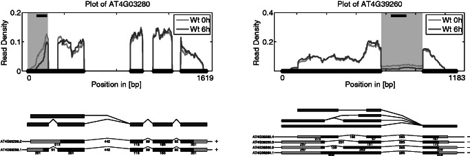
Examples of two genes detected by rDiff.nonparametric with a minimal P-value of 0.01. Shown is the read density on top. The gray area indicates the region in which the change was detected, and the black bar in the upper part of the plot shows the 100-bp region which showed the biggest difference. Below the read densities is the splice graph in dark gray and the transcripts in black. The light gray indicates the UTRs.

These results suggest that the predictions by rDiff.nonparametric can indeed be used to obtain an unbiased view with respect to alternative splicing, without annotation bias. Overall, we found that ∼60% of the detected genes had only one transcript annotated. Furthermore, we performed a classification of the events found by rDiff.nonparametric by the type of region where the biggest change was observed. The exact technical details of this annotation step are described in Supplementary Section S5.6. The result of the classification of the changes between 0 h and 1 h can be found in Figure 7 and Supplementary Table S1. In particular, changes in the 3′-UTR, 5′-UTR and introns were overrepresented (see Figure 6 for examples). As the libraries were prepared in parallel using the same reagents, we are confident that the observed coverage differences reflect the changes of the transcripts structure.

Figure 7.

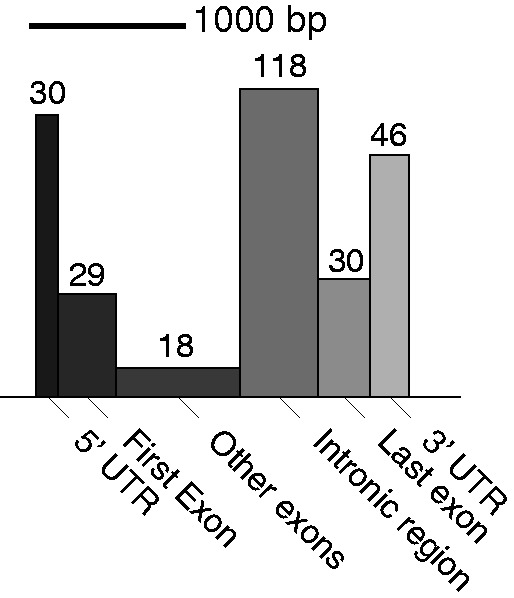
Categorization of the most differential 100 bp between the time points 0 h and 1 h according to the gene structure, in genes detected by rDiff.nonparametric with an FDR smaller than 10%. The width of the boxes is the average length of those regions, and the area equals the total number of detected differential cases.

RT–qPCR validation

To have an objective comparison on real data, we measured relative isoform levels using RT–qPCR for five genes in the three samples. This validation allowed us to verify whether the isoforms predicted to be differentially expressed have indeed a varying abundance. The protocol is described in Supplementary Section S5.4.

As a measure of correspondence between the P-value and the fold-change we used Spearman’s correlation between the negative log-P-value and the log-fold-change. We chose this correlation measure, as it is invariant under monotone transformation. We removed one outlier that led to an overly optimistic correlation for all methods. We have found a good correlation of 0.84 for rDiff.parametric, 0.68 for cuffDiff and 0.66 for rDiff.nonparametric (Figure 5). These correlations are well in line with the results on the artificial data set and support that the proposed methods retrieve accurate results.

Figure 5.

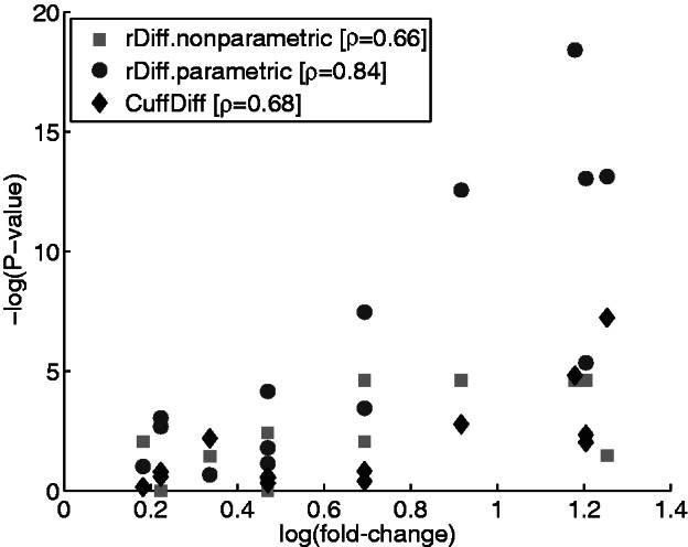
Plot of the −log(P-value) against the log(fold-change) measured by RT-qPCR. The P-values for rDiff.nonparametric are shown in light gray, for rDiff.parametric in dark gray and for CuffDiff in black. Spearman’s correlation coefficient ρ for the two methods is given in the legend.

Differential RNA processing in D. melanogaster

We also analyzed a D. melanogaster data set presented and thoroughly analyzed previously (30). It consists of two samples, one from wild-type and the other from Pasilla knockdown mutant flies, each containing two paired-end libraries and one single-end library. The authors derived multiple read counts for different types of alternative splicing events (exon skipping, intron retention and so forth) and used Fisher’s exact test (corrected P ≤ 0.05) to find significant differences in the contingency tables for the two libraries [methodology conceptually similar to a previous study (31)]. Differential splicing in 323 genes was found to be significantly different, of which 16 were experimentally validated.

We applied rDiff.parametric and rDiff.nonparametric (FDR 0.1) after aligning the reads from the paired-end libraries using TopHat (32) (more details in Supplementary Section S6). To have a small variance in the samples, we chose to exclude the single-end libraries from our analysis. Overall, rDiff.parametric and rDiff.nonparametric found 71 and 278 genes with differential relative isoform expression, respectively. Although it is reassuring that the numbers are somewhat similar, the degree calibration of the methods, including the one from Brooks et al. (30), will significantly influence the number of detected events. We, therefore, concentrated on the top 323 genes [the number of significant events found in Brooks et al. (30)]. We find that of the 16 cases that were experimentally validated previously (30), rDiff.parametric found 12 and rDiff.nonparametric found 11 genes. For three of the remaining genes, the read coverage was too low to detect significant changes for both of our methods because of the strict alignment settings used and using only the paired-end libraries. Nonetheless, the fact that rDiff.nonparametric found a large fraction of the cases is noteworthy, as it does not make use of the gene annotation.

DISCUSSION AND CONCLUSIONS

Our results on the artificial data and the study on A. thaliana and on D. melanogaster show that the proposed one-step methods outperform alternative approaches and are generally applicable. We believe that one reason that the methods perform better in practice is due to fewer assumptions made compared with other methods. In particular, quantification of alternative isoforms is a challenging task, and the predictions are often unstable and suffer from multiple possible solutions. As a consequence, the achieved FDRs are typically higher, in particular for highly confident cases. On the contrary, the proposed methods are simple, robust and can operate in complex settings while yielding statistically better calibrated estimates than other methods.

Notably, this high level of accuracy extends to the cases where genome annotations are missing. In these settings, existing quantification-based methods cannot be applied at all; hence, for the first time, we provide a workable and sufficiently accurate approach to deal with these instances. In particular, the non-parametric version of rDiff will facilitate early quantitative characterizations of transcriptomes of newly sequenced species. This finding also highlights the value of non-parametric methods that extend beyond classical uni-variate tests, such as Kolmogorov–Smirnov or the Mann–Whitney U test. rDiff.nonparametric is implemented in a flexible manner and can be used to incorporate additional features to assess the differential behavior, such as splice site or paired-end information.

We would like to note that the proposed rDiff.nonparametric method was designed to test for differential relative isoform expression. However, the method solves a more general problem ubiquitous in deep sequencing data analysis. It detects differential read coverages or other read-dependent properties that are the result of biological circumstances that one has set out to understand. For instance, the method may also be applicable for analysis of data from RNA structure probing (33,34), ChIP-seq for differential chromatin binding in different samples (G. Schweikert, personal communication) and whole-genome sequencing for testing of highly polymorphic regions (D. Weigel, personal communication). However, accounting for confounding factors in those analyses is topic of ongoing research.

In summary, we have proposed two complementary statistical tests to detect differential isoform abundances from RNA-Seq. We have shown that the methods perform better than other quantification-based methods and yield reliable predictions of differential relative isoform expression. These tools can be used in a wide range of settings, using existing gene model annotations or solely the observed read data. The NB-based rDiff.parametric test performs considerably better than the rDiff.Poisson test, as it takes the biological variance into account. The rDiff.nonparametric test is based on permutations, and taking biological variance into account is technically less straightforward. We developed the method of limited re-sampling to match the sampling variance to the biological variance. The resulting algorithm rDiff.nonparametric is significantly more robust against biological variability. Our experiments underline that biological replicates are an essential prerequisite to accurately estimate significance levels. Therefore, we advocate measurement of at least two biological replicates to estimate the variance function. Additionally, we recommend using the same sequencing method, as well as the same mapping method, to reduce systematic biases, which could lead to many false positives.

SUPPLEMENTARY DATA

Supplementary Data are available at NAR Online: Supplementary Table 1, Supplementary Figure 1 and Supplementary Methods.

FUNDING

Volkswagen foundation and Marie Curie FP7 fellowship (OS); German Research Foundation [WA2167/4-1 to A.W. and L.H.; RA1894/1-1 and RA1894/2-1 to G.R. and P.D.]; Emmy Noether fellowship [WA2167/2-1 to A.W.]. MSKCC Center for Translational Cancer Genomic Analysis [U24 CA143840 to P.D. and A.K.]; Sloan-Kettering Institute core funding (to G.R., P.D., A.K.). Funding for open access charge: German Research Foundation [RA1894/2-1].

Conflict of interest statement. None declared.

REFERENCES

- 1.Wang Z, Gerstein M, Snyder M. RNA-Seq: a revolutionary tool for transcriptomics. Nat. Rev. Genet. 2009;10:57–63. doi: 10.1038/nrg2484. [DOI] [PMC free article] [PubMed] [Google Scholar]
- 2.Mortazavi A, Williams BA, McCue K, Schaeffer L, Wold B. Mapping and quantifying mammalian transcriptomes by RNA-Seq. Nat. Methods. 2008;5:621–628. doi: 10.1038/nmeth.1226. [DOI] [PubMed] [Google Scholar]
- 3.Marioni J, Mason C, Mane S, Stephens M, Gilad Y. RNA-seq: an assessment of technical reproducibility and comparison with gene expression arrays. Genome Res. 2008;18:1509–1517. doi: 10.1101/gr.079558.108. [DOI] [PMC free article] [PubMed] [Google Scholar]
- 4.Wang L, Feng Z, Wang X, Wang X, Zhang X. DEGseq: an R package for identifying differentially expressed genes from RNA-seq data. Bioinformatics. 2010;26:136–138. doi: 10.1093/bioinformatics/btp612. [DOI] [PubMed] [Google Scholar]
- 5.Robinson MD, Smyth GK. Moderated statistical tests for assessing differences in tag abundance. Bioinformatics. 2007;23:2881–2887. doi: 10.1093/bioinformatics/btm453. [DOI] [PubMed] [Google Scholar]
- 6.Robinson M, Oshlack A. A scaling normalization method for differential expression analysis of RNA-seq data. Genome Biol. 2010;11:R25. doi: 10.1186/gb-2010-11-3-r25. [DOI] [PMC free article] [PubMed] [Google Scholar]
- 7.Anders S, Huber W. Differential expression analysis for sequence count data. Genome Biol. 2010;11:R106. doi: 10.1186/gb-2010-11-10-r106. [DOI] [PMC free article] [PubMed] [Google Scholar]
- 8.Hardcastle T, Kelly K. baySeq: empirical Bayesian methods for identifying differential expression in sequence count data. BMC Bioinformatics. 2010;11:422. doi: 10.1186/1471-2105-11-422. [DOI] [PMC free article] [PubMed] [Google Scholar]
- 9.Jiang H, Wong W. Statistical inferences for isoform expression in RNA-Seq. Bioinformatics. 2009;25:1026–1032. doi: 10.1093/bioinformatics/btp113. [DOI] [PMC free article] [PubMed] [Google Scholar]
- 10.Bohnert R, Rätsch G. rQuant.web: a tool for RNA-Seq-based transcript quantitation. Nucleic Acids Research. 2010;38:W348–W351. doi: 10.1093/nar/gkq448. [DOI] [PMC free article] [PubMed] [Google Scholar]
- 11.Griebel T, Zacher B, Ribeca P, Raineri E, Lacroix V, Guig R, Sammeth M. Modelling and simulating generic RNA-Seq experiments with the flux simulator. Nucleic Acids Res. 2012;40:10073–10083. doi: 10.1093/nar/gks666. [DOI] [PMC free article] [PubMed] [Google Scholar]
- 12.Richard H, Schulz MH, Sultan M, Nurnberger A, Schrinner S, Balzereit D, Dagand E, Rasche A, Lehrach H, Vingron M, et al. Prediction of alternative isoforms from exon expression levels in RNA-Seq experiments. Nucleic Acids Res. 2010;38:e112. doi: 10.1093/nar/gkq041. [DOI] [PMC free article] [PubMed] [Google Scholar]
- 13.Katz Y, Wang E, Airoldi E, Burge C. Analysis and design of RNA sequencing experiments for identifying isoform regulation. Nat. Methods. 2010;7:1009–1015. doi: 10.1038/nmeth.1528. [DOI] [PMC free article] [PubMed] [Google Scholar]
- 14.Glaus P, Honkela A, Rattray M. Identifying differentially expressed transcripts from RNA-seq data with biological variation. Bioinformatics. 2012;28:1721–1728. doi: 10.1093/bioinformatics/bts260. [DOI] [PMC free article] [PubMed] [Google Scholar]
- 15.Lacroix V, Sammeth M, Guigo R, Bergeron A. Exact transcriptome reconstruction from short sequence reads. In: Crandall KA, Lagergren J, editors. Algorithms in Bioinformatics. Vol. 5251 of Lecture Notes in Computer Science. Berlin Heidelberg: Springer; 2008. [Google Scholar]
- 16.Hiller D, Jiang H, Xu W, Wong W. Identifiability of isoform deconvolution from junction arrays and RNA-Seq. Bioinformatics. 2009;25:3056–3059. doi: 10.1093/bioinformatics/btp544. [DOI] [PMC free article] [PubMed] [Google Scholar]
- 17.Anders S, Reyes A, Huber W. Detecting differential usage of exons from RNA-seq data. Genome Res. 2012;22:2008–2017. doi: 10.1101/gr.133744.111. [DOI] [PMC free article] [PubMed] [Google Scholar]
- 18.Stegle O, Drewe P, Bohnert R, Borgwardt K, Rätsch G. Statistical tests for detecting differential RNA-transcript expression from read counts. Nat. Prec. 2010 doi:10.1038/npre.2010.4437.1. [Google Scholar]
- 19.Singh D, Orellana CF, Hu Y, Jones CD, Liu Y, Chiang DY, Liu J, Prins JF. FDM: a graph-based statistical method to detect differential transcription using RNA-seq data. Bioinformatics. 2011;27:2633–2640. doi: 10.1093/bioinformatics/btr458. [DOI] [PMC free article] [PubMed] [Google Scholar]
- 20.Robinson M, McCarthy D, Smyth G. edgeR: a Bioconductor package for differential expression analysis of digital gene expression data. Bioinformatics. 2010;26:139–140. doi: 10.1093/bioinformatics/btp616. [DOI] [PMC free article] [PubMed] [Google Scholar]
- 21.Loader C. locfit: local regression, likelihood and density estimation. 2007 R package. [Google Scholar]
- 22.Bonferroni C. Teoria statistica delle classi e calcolo delle probabilit. Pubblicazioni del R Istituto Superiore di Scienze Economiche e Commerciali di Firenze. 1936;8:3–62. [Google Scholar]
- 23.Gretton A, Borgwardt K, Rasch M, Schölkopf B, Smola A. A kernel method for the two-sample-problem. In: Schölkopf B, Platt J, Hofmann T, editors. Advances in Neural Information Processing Systems 19: Proceedings of the 2006 Conference. Cambridge: MIT Press; 2007. pp. 513–520. [Google Scholar]
- 24.Borgwardt K, Gretton A, Rasch M, Kriegel H, Schölkopf B, Smola A. Integrating structured biological data by kernel maximum mean discrepancy. Bioinformatics. 2006;22:e49–e57. doi: 10.1093/bioinformatics/btl242. [DOI] [PubMed] [Google Scholar]
- 25.Guo H, Yang H, Mockler TC, Lin C. Regulation of flowering time by Arabidopsis photoreceptors. Science. 1998;279:1360–1363. doi: 10.1126/science.279.5355.1360. [DOI] [PubMed] [Google Scholar]
- 26.Mockler TC, Guo H, Yang H, Duong H, Lin C. Antagonistic actions of Arabidopsis cryptochromes and phytochrome B in the regulation of floral induction. Development. 1999;126:2073–2082. doi: 10.1242/dev.126.10.2073. [DOI] [PubMed] [Google Scholar]
- 27.Jean G, Kahles A, Sreedharan V, De Bona F, Rätsch G. RNA-Seq read alignments with PALMapper. Curr. Protoc. Bioinform. 2010 doi: 10.1002/0471250953.bi1106s32. Chapter 11(December), Unit 11.6. [DOI] [PubMed] [Google Scholar]
- 28.Storey JD, Tibshirani R. Statistical significance for genome-wide experiments. Proc. Natl Acad. Sci. USA. 2003;100:9440–9445. doi: 10.1073/pnas.1530509100. [DOI] [PMC free article] [PubMed] [Google Scholar]
- 29.Trapnell C, Williams BA, Pertea G, Mortazavi A, Kwan G, van Baren MJ, Salzberg SL, Wold BJ, Pachter L. Transcript assembly and quantification by RNA-Seq reveals unannotated transcripts and isoform switching during cell differentiation. Nat. Biotechnol. 2010;28:511–515. doi: 10.1038/nbt.1621. [DOI] [PMC free article] [PubMed] [Google Scholar]
- 30.Brooks AN, Yang L, Duff MO, Hansen KD, Park JW, Dudoit S, Brenner SE, Graveley BR. Conservation of an RNA regulatory map between Drosophila and mammals. Genome Res. 2011;21:193–202. doi: 10.1101/gr.108662.110. [DOI] [PMC free article] [PubMed] [Google Scholar]
- 31.Wang E, Sandberg R, Luo S, Khrebtukova I, Zhang L, Mayr C, Kingsmore S, Schroth G, Burge C. Alternative isoform regulation in human tissue transcriptomes. Nature. 2008;456:470–476. doi: 10.1038/nature07509. [DOI] [PMC free article] [PubMed] [Google Scholar]
- 32.Trapnell C, Pachter L, Salzberg SL. TopHat: discovering splice junctions with RNA-Seq. Bioinformatics. 2009;25:1105–1111. doi: 10.1093/bioinformatics/btp120. [DOI] [PMC free article] [PubMed] [Google Scholar]
- 33.Kertesz M, Wan Y, Mazor E, Rinn JL, Nutter RC, Chang HY, Segal E. Genome-wide measurement of RNA secondary structure in yeast. Nature. 2010;467:103–107. doi: 10.1038/nature09322. [DOI] [PMC free article] [PubMed] [Google Scholar]
- 34.Underwood JG, Uzilov AV, Katzman S, Onodera CS, Mainzer JE, Mathews DH, Lowe TM, Salama SR, Haussler D. FragSeq: transcriptome-wide RNA structure probing using high-throughput sequencing. Nat. Methods. 2010;7:995–1001. doi: 10.1038/nmeth.1529. [DOI] [PMC free article] [PubMed] [Google Scholar]
Associated Data
This section collects any data citations, data availability statements, or supplementary materials included in this article.