A Fast Estimate for the Population Recombination Rate Based on Regression

Abstract

Recombination is a fundamental evolutionary force. Therefore the population recombination rate ρ plays an important role in the analysis of population genetic data; however, it is notoriously difficult to estimate. This difficulty applies both to the accuracy of commonly used estimates and to the computational efforts required to obtain them. Some particularly popular methods are based on approximations to the likelihood. They require considerably less computational efforts than the full-likelihood method with not much less accuracy. Nevertheless, the computation of these approximate estimates can still be very time consuming, in particular when the sample size is large. Although auxiliary quantities for composite likelihood estimates can be computed in advance and stored in tables, these tables need to be recomputed if either the sample size or the mutation rate θ changes. Here we introduce a new method based on regression combined with boosting as a model selection technique. For large samples, it requires much less computational effort than other approximate methods, while providing similar levels of accuracy. Notably, for a sample of hundreds or thousands of individuals, the estimate of ρ using regression can be obtained on a single personal computer within a couple of minutes while other methods may need a couple of days or months (or even years). When the sample size is smaller (n ≤ 50), our new method remains computational efficient but produces biased estimates. We expect the new estimates to be helpful when analyzing large samples and/or many loci with possibly different mutation rates.

IN diploid organisms, recombination mixes the maternal and paternal genetic material during meiosis, leading to differently composed gametes. From a population genetic point of view, recombination is an essential evolutionary force. It produces new haplotypes and increases the genetic variation in a population, by breaking up the linkage between genes.

At the population level, recombination occurs at a certain frequency, the population recombination rate (usually denoted by ρ = 4Nr, where N is the effective population size, and r the recombination rate per locus). The population recombination rate affects the extent of linkage disequilibrium (LD) (Hill 1968), and estimates of ρ are important in the study of the evolutionary history of a population. Since positive selection also affects the LD, estimates of ρ are helpful when looking for traces of positive selection (Sabeti et al. 2002, 2006). They also play an important role in genome-wide association studies (Pritchard and Przeworski 2001).

Classic methods of estimating ρ include the computation of a lower bound on the number of recombination events (Hudson and Kaplan 1985; Wiuf 2002; Myers and Griffiths 2003), moment estimation (Hudson 1987; Wakeley 1997; Batorsky et al. 2011), composite likelihood estimation (Hey 1997; Hudson 2001; McVean et al. 2002; Wall 2004; Chan et al. 2012), likelihood methods based on summary statistics (Wall 2000; Li and Stephens 2003), and full-likelihood estimation (Kuhner et al. 2000; Fearnhead and Donnelly 2001). Since likelihood methods use all available information, their accuracy is usually higher than that of the other methods that are based on less information. On the other hand, they require considerably higher computational efforts. Indeed, full-likelihood estimation usually requires the use of strategies such as Markov chain Monte Carlo (Kuhner et al. 2000) or importance sampling (Fearnhead and Donnelly 2001), to be computationally feasible. These computational techniques lead again to approximations to the actual maximum-likelihood estimates. Although considerable efforts have been put into composite likelihood methods (Fearnhead and Donnelly 2002; Wall 2004), they are still highly computationally demanding. Therefore, lookup tables are often used to avoid the need for repeating time-consuming likelihood computations, when recombination needs to be estimated for several positions at which both sample size and the scaled mutation parameter θ are equal. Especially for larger sample sizes, the generation of lookup tables may well take several months (see Table 4). Another method that uses summary statistics for estimating ρ has been proposed by Wall (2000). There ρ is estimated by approximating the likelihood of suitably chosen summary statistics via simulations. A further competitive approach has been proposed in Li and Stephens (2003). It is based on splitting the likelihood into approximate conditional distributions. These methods perform not much worse than likelihood methods using the full information but at a lower computational effort.

Table 4. A time study for different methods.

Method	n = 50	n = 100	n = 200
gam	<5 min	<5 min	<5 min
SSL	4 days	6 days	7 days
LDhat	1 day	20 days	499 days
PAC	3 hr	11 hr	35 hr

The table shows the computing time for the four methods to analyze 100 SNP data sets. For boosting, this was the time needed for simulation, the summary statistics computation, training, and estimating. For SSL, this involved the time for simulation, summary statistics computation, the likelihood computation, and estimating. For LDhat and PAC, it was the time required for simulation, the likelihood computation, and estimating. For boosting, LDhat, and SSL, the steps before estimating were run once and the results were used to estimate ρ for 100 test data sets. For PAC, each testing sample was handled separately by HOTSPOTTER. All these programs/scripts were run on a Linux cluster. For SSL and LDhat, each job was divided into hundreds of parallel running parts and the time in this table was the total time summed over all parts. Because of varying workloads of the cluster, the table provides only an approximate computation time that might be slightly different for a different run.

In this study, we propose a new regression-based estimate of ρ that is very fast to compute. As explanatory variables, we use summary statistics, and ρ is our dependent variable. Depending on which and how many summary statistics are used, several regression models are possible. Ideally, the regression model that optimizes the predictive accuracy should be chosen. A promising method for estimating the best possible model is boosting (Bühlmann and Hothorn 2007), a machine learning method, which can be used both for classification and regression. In another population genetic setup, Lin et al. (2011) implemented boosting successfully to distinguish positive selection and neutral evolution, by solving a binary classification problem.

When the sample size is not small (n ≥ 100), our simulation results show that our method leads to a level of accuracy similar to that achievable with composite likelihood and summary statistic-based likelihood. The amount of computational effort, however, is much smaller with our proposed method. When the sample size is smaller (n ≤ 50), our new method remains computational efficient but produces biased estimates. This makes our proposed regression approach particularly useful for large samples.

Methods

Regression and boosting

A common statistical goal is to predict a response Y (one dimension) such as the recombination rate from a k-dimensional vector of predictors X.

In machine learning, a set of training samples with known values for X and Y can be used to study the relationship between X and Y. This is called the training process. Training leads to a model Y = f(X) + ε, which can be used to predict Y from X in new samples. If Y is a binary variable, taking only the values 0 and 1, this is called classification. If Y is a continuous variable, this is a regression problem.

Here we applied boosting, a machine learning method (Bühlmann and Hothorn 2007) that tries to find out iteratively the model Y = f(X), which fits the training data best. Our focus is on L₂ boosting (Bühlmann and Hothorn 2007) with the goal to estimate

$$f^{*}(\cdot )={\text{argmin}}_{f\in ℱ}E{\left(Y-f\left(X\right)\right)}^2,$$

i.e., the best approximating function within the class ℱ of functions. As function classes ℱ, we considered both the class of linear functions $f_{\beta }\left(x_1,\dots ,x_k\right)={\beta }_0+{\displaystyle {\sum }_{i=1}^k{\beta }_i{x}_i}$ and the class of additive models based on smoothing splines $f_h\left(x_1,\dots ,x_k\right)={\beta }_0+{\displaystyle {\sum }_{i=1}^k{h}_i\left(x_i\right)}$. Here h = (h₁,…,h_k) are cubic spline functions that adapt well to any kind of nonlinear relationship.

The boosting algorithm adjusts the model gradually to fit the training data better. The number of adjustment steps is the main tuning parameter. The more steps are taken, the better the model fits the training data. Too many steps, on the other hand, can lead to overfitting.

As described in Bühlmann and Hothorn (2007), this is achieved by starting with the best possible constant fit $f^{\left[0\right]}\left(x_1,\dots ,x_k\right)=\left(1/l\right){\displaystyle {\sum }_{i=1}^l{Y}_i}$ to the simulated training data consisting of l cases. Then at step m + 1 a simple base procedure is fitted to the residuals $U^{\left[m\right]}=\left(u_1^{\left[m\right]},\dots ,u_n^{\left[m\right]}\right)$ from step m, with $u_j^{\left[m\right]}=Y_j-f^{\left[m\right]}\left(x_{1j},\dots ,x_{kj}\right)$. In the case of a linear function class (glmboost), the base procedure computes a linear fit to the residuals using the best fitting explanatory variable. In more detail, let X_i = (x_i1, …, x_il) denote the data on explanatory variable i (1 ≤ i ≤ k). We add X₀ ≡ 1 represents the constant term. Then

$${\widehat{\beta }}_i=\frac{X_i^t\cdot U^{\left[m\right]}}{{\Vert X_i\Vert }^2}$$

gives the regression coefficient for X_i. We now look for the best-fitting predictor

$$b:={\text{argmin}}_{0\le i\le k}{\displaystyle \sum _{j=1}^l{\left(u_j^{\left[m\right]}-{\widehat{\beta }}_i{x}_{ij}\right)}^2}$$

and update the regression function

$${\widehat{f}}^{\left[m+1\right]}\left(x_1,\dots ,x_k\right)={\widehat{f}}^{\left[m\right]}\left(x_1,\dots ,x_k\right)+\nu {\widehat{\beta }}_b{x}_b.$$

Here, ν ≤ 1 is a step-length parameter. We also update the corresponding coefficient ${\widehat{\beta }}_b^{\left[m+1\right]}={\widehat{\beta }}_b^{\left[m\right]}+\nu {\widehat{\beta }}_b$ and leave all other regression coefficients unchanged. (Since it is usually advisable to choose ν < 1, and since the explanatory variables will usually not be independent, the same coefficient will in general be updated several times during the iteration process.) Boosting with additive models works analogously, but more flexible spline functions are taken to fit the residuals.

We used the boosting algorithm implemented in the R package mboost (Hothorn and Bühlmann 2002). L₂-boosting is available there both for generalized linear model regression (glm-boosting or short glm) and for generalized additive models based on splines (gam-boosting or short gam) We used both methods with the default parameters. Note that glm is also capable of estimating generalized linear models (for instance, for binomial responses), but we chose the default Gaussian family with identity link, which leads to a base procedure that applies ordinary linear models.

Although it is known that boosting is fairly resistant against overfitting (Bühlmann and Hothorn 2007), a proper stopping rule is helpful for choosing an appropriate model. The package mboost provides both AIC and cross-validation-based methods for this purpose. Here, we used a modified version of Akaike’s information criterion (AIC) (Akaike 1974; Bühlmann 2006) since it is faster than cross-validation and led to similar levels of accuracy in our situation. The criterion is available as part of the mboost package (function AIC with the option ”corrected”). Note, however, that AIC tends to select slightly larger models than those obtained by cross-validation, and boosting can be expected to perform even slightly better with cross-validation. By computing a model selection criterion in each iteration of the algorithm, complexity changes can be monitored. Stopping the boosting iterations when AIC or the cross-validation error is smallest is a successful strategy to prevent overfitting.

In population genetics, the objects we study are DNA samples. One sample usually contains several DNA sequences of the same (homologous) region from different individuals taken from the population of interest. To define a regression model, the predictors X can be chosen to be summary statistics computed from the DNA data. Popular summary statistics are based on the number of segregating sites, the site frequency spectrum, the LD, or the number of different haplotypes (Tajima 1989; Fay and Wu 2000; Wall 2000; Sabeti et al. 2002). In principle, the response variable Y can be any quantity that describes a certain evolutionary force. Thus, the inference of an evolutionary force can be viewed in terms of finding the best model Y = f(X) + ε. In this study, we consider the response Y to be the population recombination rate, which is a continuous variable. This explains why we use boosting in connection with regression here. In Lin et al. (2011) on the other hand, Y has been taken as a binary variable with 0 indicating neutral evolution and 1 positive selection. This led to a problem of classification.

Estimating ρ using likelihood methods

Wall (2000) took the number of different haplotypes H as a summary statistic. Given H, the likelihoods for a series of values for ρ were calculated using simulations. The value of ρ leading to the maximum simulated likelihood has been taken as the estimate. Since it is also based on summary statistics, Wall’s method is related to our approach. We therefore applied Wall’s method (summary statistic likelihood, denoted by SSL) and compared it to our method. For a given n and S and for each ρ ∈ {1, 2, 3,…,200}, we simulated 100,000 samples, where S is the number of segregating sites. Then we computed the proportion $\widehat{\text{Pr}}\left(H|\rho \right)$ of the samples with a certain number H of different haplotypes. When given a new sample with S segregating sites, we computed H* = H(S) for this sample and took the ρ with the maximum-likelihood $\widehat{\text{Pr}}\left(H^{*}|\rho \right)$ as our estimate.

Another popular approach for estimating ρ we consider here is the composite likelihood method proposed by Hudson (2001). It requires the probabilities of all two-locus sampling configurations and has been implemented in the popular software package LDhat (v. 2.1) (McVean et al. 2002). Using the complete program of LDhat, we computed the two-locus sampling configuration lookup tables for n = 50, 100, and 200 respectively. When computing the lookup tables, θ was set to 0.001 and the maximum ρ for the likelihood was set to be 200. The pairwise program was then used to estimate the population recombination rate for the region analyzed assuming a constant recombination rate over the region.

Recently, Li and Stephens (2003) introduced a product of approximate conditionals (PAC) model and provided a maximum PAC likelihood estimate for ρ. The method has also been used to identify recombination hotspots from population SNP data. We downloaded the source code of their software, HOTSPOTTER (v. 1.2.1) http://stephenslab.uchicago.edu/ compiled it for our computer cluster.

Simulation

All estimation methods we consider require at least some simulations. With boosting, we need training samples to estimate the regression relationship. When applying SSL, we also need to simulate samples to compute the likelihood. For computing composite likelihoods, importance sampling to obtain the two locus sample configurations needs to be carried out within the LDhat package. The PAC method implemented in the HOTSPOTTER softwarevrelies on numerical optimization of a simplified likelihood. The estimates produced tend to be biased, and a bias correction has been proposed that relies on simulations. Also, as the PAC likelihood depends on the ordering of the haplotypes, the software averages the estimates obtained from several random orderings, To analyze the performance of the considered methods, we independently generated testing samples and analyzed them with each method. To simulate neutral and bottleneck DNA samples, we used the program ms of Hudson (2002). To simulate selection samples, we used the program msms(Ewing and Hermisson 2010). The parameter definitions can be found in Table 1.

Table 1. Simulation parameters.

Parameter	Description
N	Number of sampled chromosomes
S	Number of segregating sites
θ	Population mutation rate for the investigated region(4Neμ)
ρ	Population recombination rate for the investigated region(4Ner)
α	(For selection samples) = 4Nes, where s is the selective coefficient
τ	(For selection samples) time when the beneficial mutation get fixed
t0	(For bottleneck samples) time when the bottleneck ended
t1	(For bottleneck samples) duration of bottleneck

N_e, the effective population size; μ, mutation rate per generation per individual within the investigated region; r, recombination rate per generation per individual within the investigated region. The time parameters (τ, t₀, t₁) are in the unit of 4N_e generations, backward in time. For the selection samples, a beneficial mutation has been simulated to occur at the center of the region. The beneficial allele frequency increases subsequently and fixation was assumed to occur at time τ. The whole region thus experienced a full, hard selective sweep. With boosting, for each value in a set of parameters, 100 replications were simulated as candidates for training, and 100 independent replications were simulated for testing (some testing samples were also used with LDhat, SSL, and PAC). One example scenario involved n = 200 with S = 59 segregating sites. Under this scenario, we simulated samples for different values of ρ. With boosting, we trained for instance under the values ρ = 20, 60, 100, 140, and 180 and estimated ρ under testing samples with values of ρ in {10, 20,…,150}. This leads to 5 × 100 = 500 training samples and 15 × 100 = 1500 testing samples (generated independently from the training samples). We used either θ or S to set the level of polymorphism, and mostly we used fixed S in our simulations.

Results

Relative importance of summary statistics and two regression models

We first consider a single locus on n chromosomes (n = 200) with a fixed S = 59. We summarize the data using 10 different summary statistics capturing effects of recombination (see Table 2 for details).

Table 2. Different statistics and their standardized coefficients estimated via a linear model selected by boosting.

Statistics	Meaning	coef
H	Number of different haplotypes	0.00
$R_{h^{*}}$	H − S (Myers and Griffiths 2003)	50.18
Rm	Minimum number of recombination events inferred from TGT (Hudson and Kaplan 1985; Gusfield 1991)	0.72
$S_k^2$	Variance of average pairwise differences for the whole region (Sved 1968; Hudson 1987)	1.78
Hetero	Haplotype heterozygosity (the probability that two segments are different in haplotype)	−0.58
pR	Proportion of SNP pairs that TGT indicates a recombination event	0.55
Mean $S_k^2$	For each SNP pair, $S_k^2$ was computed, and then the mean was computed over all SNP pairs	−3.19
Mean r2	Similar to mean $S_k^2$, but r2 was computed instead of $S_k^2$(Hudson 1985)	−3.03
Mean LD1	Similar to mean $S_k^2$, but LD1 was computed instead of $S_k^2$. LD1 is a measure of LD proposed by Batorsky et al. (2011), defined as the normalized frequency of LRH (least-represented haplotype) for a pair of SNPs.	−2.01
LD2	LD2 is a measure of LD proposed by Batorsky et al. (2011), defined as the proportion of the SNP pairs for which the frequency of LRH is below 0.04.	−0.26

TGT, three-gamete test (Gusfield 1991). We chose 10 summary statistics that are directly or indirectly related to ρ. Sample parameters: n = 200, S = 59. In the original article of Myers and Griffiths (2003), R_h is the maximum of H − S over some subsets of segregating sites. Here we computed H − S only once for the whole region, so we denoted this value as $R_{h^{*}}$ rather than R_h. coef shows the standardized linear coefficient for each statistic obtained via a linear model (glm) where we fitted all 10 statistics to predict ρ. Training was done with 5 ρ’s (20, 60, 100, 140, and 180). A large absolute value of a standardized coefficient indicates a large influence of the corresponding statistic. When fixing S, $R_{h^{*}}$ contains the same information as H. Thus boosting only selects one of them and discards the other (by assigning coefficients equal to 0).

When estimating ρ, the relative importance of the considered summary statistics is of general interest. Using boosting, the coefficients obtained from fitting a generalized linear model (glm) provide insight concerning the relative importance of the corresponding summary statistics (Table 2). When conditioning on the number of segregating sites, both H and $R_{h^{*}}$ contain exactly the same information, and boosting selected only one of them (Table 2). Furthermore, according to the estimated coefficients, either H or $R_{h^{*}}$ turn out to be much more important in estimating ρ, than all other statistics (Table 2).

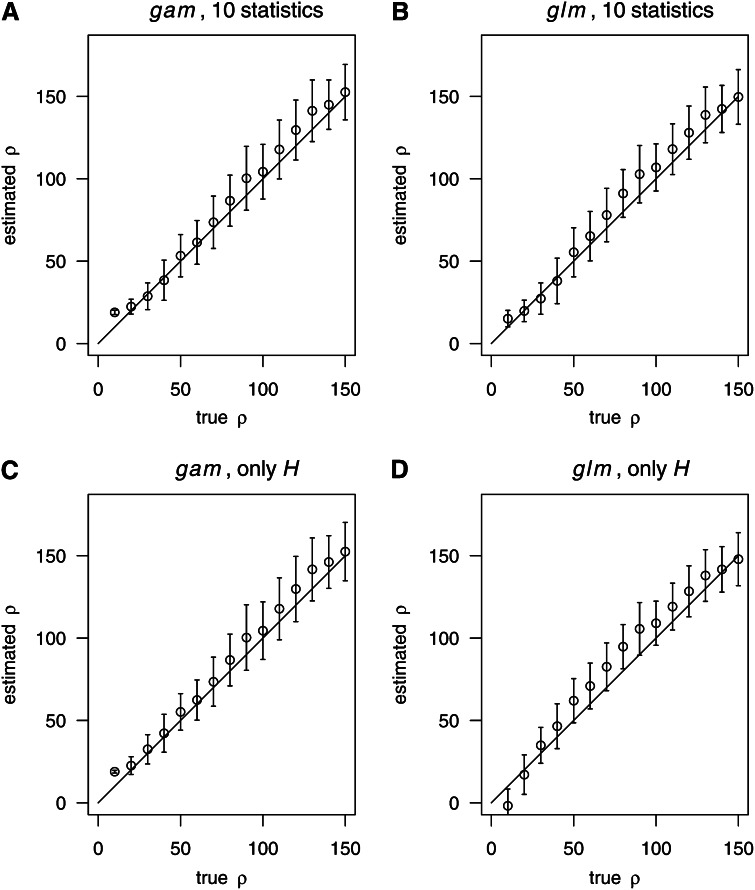
As an alternative, we used the number of haplotype (H) as the only predictor variable X. The quality of fit, both for the linear and the nonparametric model (glm and gam), is presented (Figure 1). Generally, the quality of the nonparametric estimates (gam, Figure 1, A and C) has been better than that of the linear regression (glm, Figure 1, B and D). In particular, the glm estimates had a higher bias compared to the gam estimates. This suggests a nonlinear relationship between the recombination rate and the considered summary statistics.

Figure 1.

Estimating ρ based on two different strategies for boosting. In each part (A–D), we provide averages and standard deviation bars to illustrate both bias and random errors of the estimates of ρ. A grid of true values of ρ is displayed on the x-axis. The solid line showed where estimated ρ equals real ρ. We considered the following two strategies for boosting: “10 statistics,” 10 summary statistics (Table 2) were used to represent the data. “Only H”: only the number of different haplotypes was used to represent the data. Simulation parameters: n = 200, S = 59. For training, we used ρ = 20, 60, 100, 140, and 180. For each true value of ρ, 100 samples (independent from the training samples) were used for testing.

Moreover, Figure 1 also suggests that the estimates of ρ have almost the same accuracy when using only H (Figure 1, C and D) compared to the use of all 10 statistics (Figure 1, A and B). This also agrees with the results shown in Table 2, suggesting that the number of haplotypes provides essential information for estimating ρ. Therefore we always used the nonparametric model based on H to estimate ρ by boosting in the subsequent analysis, unless mentioned.

Accuracy of boosting, LDhat, SSL, and PAC

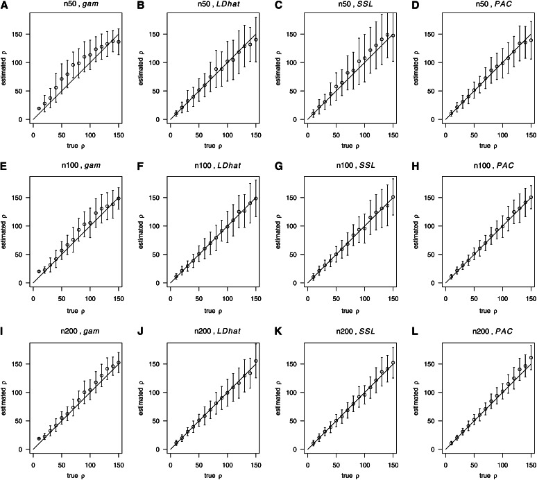
We measured the accuracy of the four considered methods using the bias and the variance (Figure 2). When the number of sampled chromosomes was small (n = 50, Figure 2, A–D), boosting produced estimates with a fairly small variance but somewhat overestimates ρ on average when ρ was intermediate. Notably, the boosting estimates are almost unbiased while having a fairly small variance when n ≥ 100 (Figure 2, E and I). A more detailed comparison of the root mean square errors of the four methods can be found in Table 3. Overall, these results suggest a comparable performance of the methods, with boosting tending to perform best for large values of ρ (Table 3).

Figure 2.

Comparison of boosting with LDhat, SSL, and PAC. We compared gam-boosting (A, E, I) with LDhat (B, F, J), SSL (C, G, K), and PAC (D, H, L), for the sample sizes n = 50 (A-D), 100 (E-H), and 200 (I-L), respectively. Further simulation parameters: S = 45 (when n = 50), 52 (when n = 100), and 59 (when n = 200). With boosting, we used r = 20, 60, 100, 140, and 180 for training.

Table 3. Root mean squared errors for different methods.

	n = 50				n = 100				n = 200
True ρ	gam	LDhat	SSL	PAC	gam	LDhat	SSL	PAC	gam	LDhat	SSL	PAC
10	9.6	4.7	6.6	4.9	10.4	5.0	5.7	4.1	8.9	4.7	4.9	3.4
20	16.5	9.5	12.7	8.3	6.1	7.8	8.1	6.4	6.0	5.7	6.8	4.5
30	18.6	18.4	13.2	11.4	12.4	9.0	9.1	7.5	9.2	7.2	7.3	6.0
40	30.1	16.8	20.1	12.9	15.2	11.9	10.7	9.0	11.7	10.1	9.7	8.5
50	33.9	19.8	25.3	14.4	17.2	14.0	13.8	10.5	12.3	10.7	10.7	9.3
60	31.0	20.4	23.2	14.5	18.3	17.6	15.7	13.6	12.4	15.9	12.0	10.8
70	34.3	26.2	32.3	18.6	22.7	19.8	19.8	13.4	15.3	15.4	13.8	10.6
80	31.7	33.9	32.9	23.6	24.1	22.4	18.8	15.0	17.1	19.0	13.8	13.5
90	33.3	30.2	42.4	23.3	25.7	18.5	22.8	16.1	22.4	20.2	18.2	14.8
100	29.2	34.9	42.4	26.0	26.6	27.5	25.8	19.0	18.1	23.6	16.8	13.7
110	25.7	35.0	41.9	27.0	28.2	27.5	30.3	21.7	20.4	24.4	18.9	17.1
120	23.6	37.6	42.4	26.7	27.0	29.0	31.4	21.5	22.1	26.8	22.2	19.6
130	22.1	36.7	45.4	31.0	24.2	29.1	33.4	25.1	22.4	28.5	25.7	22.1
140	18.9	31.1	41.5	28.3	24.4	34.7	36.2	24.9	17.2	27.1	23.5	20.6
150	26.4	40.1	45.3	34.9	18.8	32.2	31.8	20.2	17.9	30.4	27.0	23.9

The table contains the root mean squared errors of four different estimators (gam-boosting, LDhat, SSL, and PAC) of ρ under the setup of Figure 2.

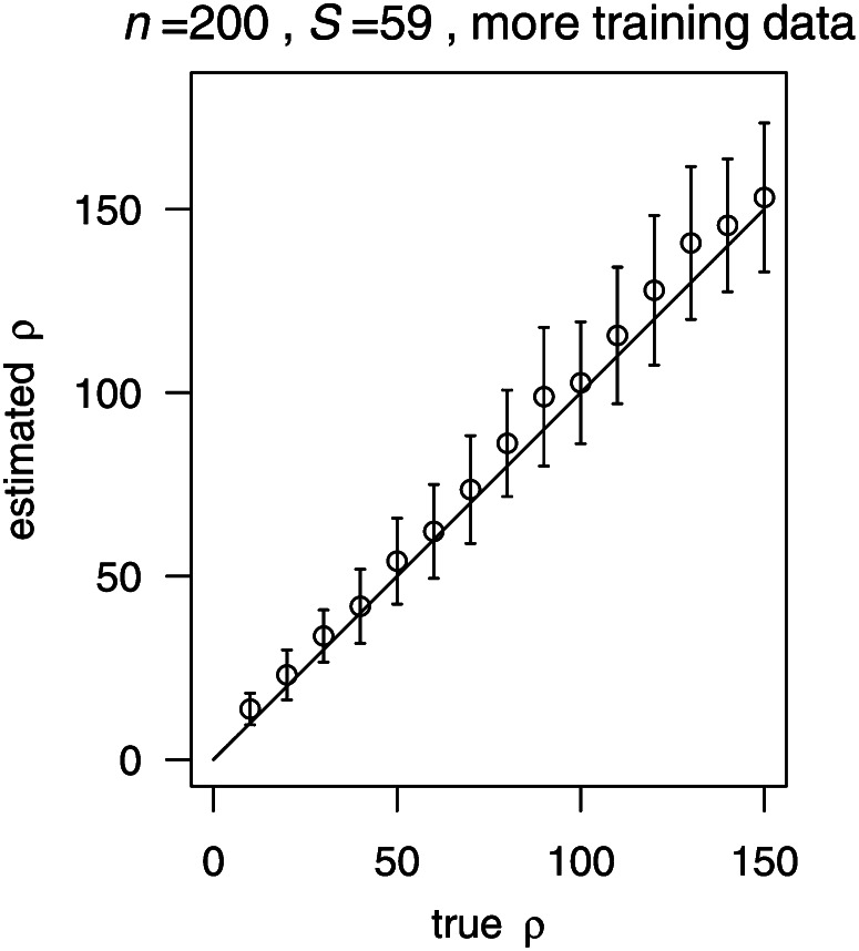
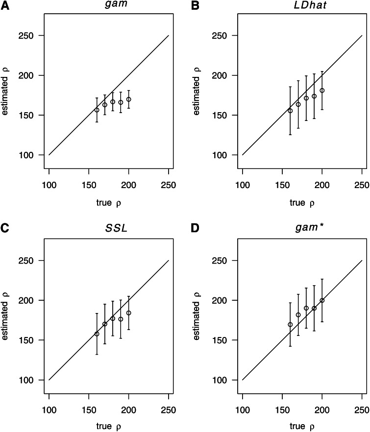
Importantly, boosting can lead to biased estimates if the true value of ρ does not fall into the range of the training parameters (here: [20, 180]). For example, when the true value of ρ is 10, boosting slightly overestimates ρ (Figure 2, E and I). However, if the range of the training parameters does cover the value 10, the estimate becomes unbiased (Figure 3). Similarly, if the true ρ exceeds the maximum value of the training parameters, boosting tends to underestimate ρ (Figure 4A). This can again be mostly avoided by enlarging the range of training values (Figure 4D). Note, however, that the estimation problem is more difficult when ρ is large. Indeed, also the likelihood methods (LDhat and SSL) showed some bias in this case (Figure 4, B and C).

Figure 3.

Influence of the number of different training scenarios on the accuracy of the estimates of ρ obtained from gam-boosting. The parameters in this figure were the same as that in Figure 1C. Instead of training with 5 ρ’s (20, 60, 100, 140, and 180), the training was done with 20 ρ’s (10, 20, …, 200).

Figure 4.

Estimation when ρ is large. Estimation of ρ for true values in the range [160, 200]. n = 200, S = 59. (A) gam-boosting, with training under ρ = (20, 60, 100, 140, 180); (B) LDhat; (C) SSL; (D) gam-boosting, with training under ρ = (20, 60, 100, 140, 180, 220, 260).

We also examined whether more training data help to improve the quality of estimation. The boosting estimates presented above were obtained by training under only 5 values of ρ (20, 60, 100, 140, 180) and testing with 15 ρ’s (10, 20, …, 150). To investigate this further, we used a larger training sample that involves 20 values of ρ. However, the variance of the estimates remained similar (Figure 3) compared with the results from training only under 5 values for ρ (Figure 1C). Therefore, a fairly sparse training data set seems to be sufficient with boosting.

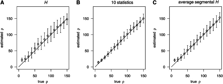
We examined further cases with a very high level of polymorphism (S > n). We found that the variance of the boosting estimate slightly increased (Figure 5A) when only the summary statistic H was used. An explanation is that when S is large, H is more likely to hit its bound n, thus leading to a loss of information carried by the statistic. This observation fits also to the observation of a reduced importance of H relative to other summary statistics when the polymorphism level was very high (Supporting Information, Table S1).

Figure 5.

Boosting algorithm when polymorphism level is high. For all the samples in this figure, n = 200 and S = 294. (A) Using only H as explanatory variable. (B) Using all 10 summary statistics (Table 2) as explanatory variables. (C) The whole section was cut up into five segments of equal length and the number of different haploptype was computed in each segment. Then the average segmental H was used.

We see two strategies for handling cases with a high level of polymorphism. One is to use further summary statistics besides H (Figure 5B) as they are more informative when polymorphism is high (Table S1). However, the use of more statistics requires additional computations for each simulated training data set. Another remedy is to cut up the whole region under investigation into several smaller DNA segments. The number of haplotypes H can then be computed separately for each segment. The average over the segmental values of H may then be used as a single summary statistic for a sample (Figure 5C). When choosing the segments such that the number of segregating sites within each segment is not too large, this strategy worked very well both with respect to computation time and accuracy.

Not surprisingly, a larger sample size (n = 1000, S = 75, Figure S1A) helps to reduce the variance of all estimates of ρ. The situation where both the sample size and the level of polymorphism were large (n = 1000, S = 374, Figure S1B) led to the best estimates, although the gain achieved under a larger value of S was not huge.

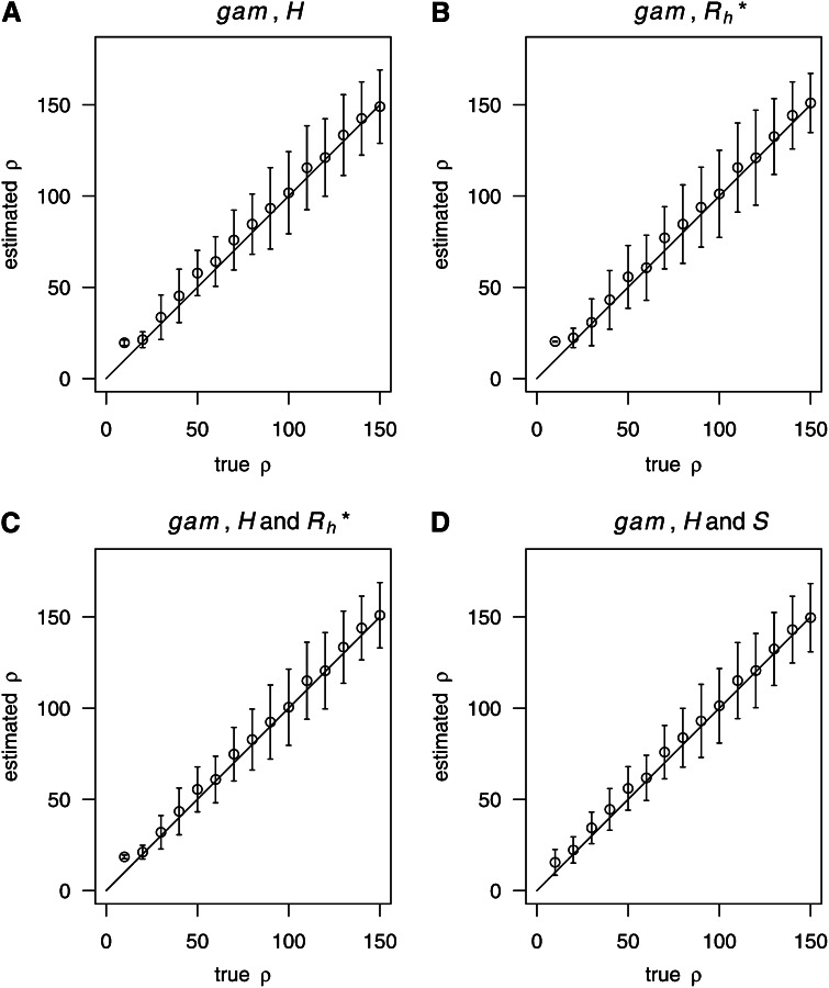
Generally speaking, it is natural to train boosting conditional on the number of segregating sites S . However, in population genetics, it is common practice to simulate data given θ. Therefore, we also investigated the effect on the estimation quality when fixing θ in both training and testing samples. We tried using only H (Figure 6A), only $R_{h^{*}}$ (Figure 6B), H and $R_{h^{*}}$ (Figure 6C), and H and S (Figure 6D), respectively, to represent the samples. The results remained good (Figure 6). In principle, $R_{h^{*}}$ should be more suitable than H in such circumstances, since H will be directly affected by the random number of segregating sites S. However, in our examined cases H still worked as well as $R_{h^{*}}$ (Figure 6).

Figure 6.

Estimating ρ with training under a fixed value of θ. Estimation of ρ when fixing θ instead of S for training and testing. n = 200, θ = 10. (A) Using only H. (B) Using only $R_{h^{*}}$. (C) Using H and $R_{h^{*}}$. (D) Using H and S.

Computational cost of boosting, LDhat, SSL, and PAC

We now turn to a comparison of the computational efforts required with our considered methods (Table 4). We focus on the scenarios underlying the results in Figure 2. It turns out that the computations involved with boosting require much less time than for the other three methods. This is particularly important with large samples, where other methods become highly computationally demanding. Indeed, when the number of sampled chromosomes has been large (n ≥ 200), the computation time required by LDhat has been much longer than with boosting (several months vs. several minutes). Notably, even when n = 1000, boosting needs only ∼4 min (<5 min, result not shown in Table 4) to analyze 100 data sets. Moreover, the largest part of the time required for boosting turned out to be for the model selection during the training process. Without the model selection step involving AIC, the computation time for simulation, computing summary statistics, and gam training was <1 min for the cases in Table 4. Since boosting is fairly resistant to overfitting, it would actually be sufficient to compute the AIC on a rather sparse grid, and computation times between the stated values of 1 and 5 min seem realistic.

A look at the other methods revealed that SSL needed a lot of time for the simulations (Table 4). For each ρ ∈ {1, 2, …, 200}, we simulated 100,000 replications as recommended by Wall (2000). Boosting, in comparison, required only 5 ρ’s and 100 replications for each ρ for the training process, to lead to good performance. This explains the much higher speed of boosting.

It should be noted that the time required by LDhat increases dramatically with the sample size. Indeed, the computation of the look-up table for LDhat (to compute composite likelihood) took almost 500 days for a sample of size 200 without parallel computing. The computation time needed with the PAC approach was considerably below that for LDhat and SSL, but still considerably above that with boosting. It increased approximately quadratically with the sample size, so boosting seems attractive, especially with large samples.

Indeed, boosting can easily and promptly handle cases with a very large sample size (n = 1000, Figure S1) within several minutes using a single PC: such sample sizes exceed the handling ability of LDhat, even with the support of a modern computer cluster (∼800 CPUs).

Robustness against selection and demography

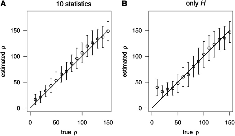
Recently, Reed and Tishkoff (2006) found that positive selection can create false hotspots of recombination, if ρ is estimated based on the pattern of linkage disequilibrium (Li and Stephens 2003). Unlike the LD-based method, our method is generally robust to the effect of positive selection. When all 10 summary statistics (Table 2) were used, positive selection did not affect the quality of estimating ρ (Figure 7A). When the data were summarized by the number of haplotypes only, positive selection somewhat affects our estimates of recombination (Figure 7B). However, this effect can be seen only on a narrow surrounding region of the beneficial allele (i.e., where ρ ≤ 30, representing ∼10 kb since ρ [per kilobase] is 3 here). The effect can be understood as follows: we simulated the hitchhiking data given the number of segregating sites, and selection may result in an excess of haplotypes relative to what is expected from the number of segregating sites, as indicated by negative F’s (Fu 1997).

Figure 7.

Estimating ρ in selection samples. Estimation of ρ in selection samples. n = 200, S = 59. Selection parameters: α = 500, τ = 0.001. (A) Using 10 statistics (Table 2). (B) Using only H. The samples used for training (i.e., regression) and testing were both selection samples with the same parameters.

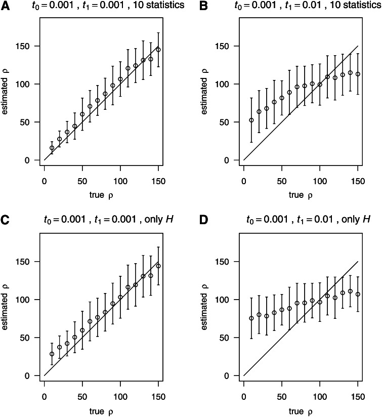
We also examined the robustness of estimates of ρ under various bottleneck scenarios (Figure 8). Please refer to Table 1 for the parameters of the simulated bottleneck samples. It should be noted that the average $\widehat{\rho }$ may not be equal to ρ_true in a varying size population since $\widehat{\rho }\approx 4\overline{N}r$, where $\overline{N}$ represents a long term effective population size, and ρ_true = 4N₀r, where N₀ is the current effective population size. Generally, $\overline{N}\ne N_0$, so $\widehat{\rho }\ne {\rho }_{\text{true}}$. When the 10 summary statistics were used, the examined bottleneck scenarios (including weak and strong bottlenecks) had less effect than when only the number of haplotypes was considered. In the latter case with a severe bottleneck (Figure 8D), overestimation occurred in regions with low recombination. The overestimation is due to an increase in the number of haplotypes (given the fixed number of segregating sites in simulations), because of an excess of rare mutations (results not shown) caused by the severe bottleneck. In regions with high recombination rate, the recombination rate might be underestimated because rare mutations contain less information about recombination events. However, the observed pattern under bottleneck scenarios does not cause false positives when inferring recombination hotspot.

Figure 8.

Estimating ρ in bottleneck samples. Estimation of ρ in bottleneck samples. n = 200, S = 59. the population size during bottleneck is 0.01N₀, where N₀ is the population size before and after bottleneck. (A) Using 10 statistics (Table 2), t₀ = 0.001, t₁ = 0.001. (B) Using 10 statistics, t₀ = 0.001, t₁ = 0.01. (C) Using only H, t₀ = 0.001, t₁ = 0.001. (D) Using only H, t₀ = 0.001, t₁ = 0.01. The samples used for training (i.e., regression) and testing were both bottleneck samples with the same parameters.

We note that boosting is simulation based, and simulations generally have been performed with a fixed number of segregating sites (S). To improve the precision of the estimate of ρ under a varying size population, the simulations could also be performed conditional on the observed mutation frequency spectrum. By conditioning on the observed mutation frequency spectrum, one may be able to solve the difficulties caused by the excess/deficiency of haplotypes in a varying size population. This feature will be investigated further and included with the release of the software to our approach.

Discussion

In the genomic era, our ability of data generation may soon surpass that of data analysis. It can be expected that we will soon be able to sequence thousands of individuals of an investigated species at low cost and within a short period of time. For humans this has already started to become reality (http://www.1000genomes.org) (1000 Genomes Project Consortium 2010). Thus it will be important to also analyze a large amount of data promptly and precisely.

In this study, we propose boosting as an approach to selecting an appropriate regression model for estimating the population recombination rate ρ, an important quantity in population genetics. Especially for large samples, our proposed method achieves a similar level of accuracy as competing methods (Wall 2000; McVean et al. 2002; Li and Stephens 2003), but at much lower computational effort. Thus boosting provides an attractive approach to obtain estimates of the population recombination rate ρ with large samples.

Boosting is a machine learning method for which an appropriate range of training values for ρ needs to be chosen. Here, care should be taken to ensure that the true ρ falls within the range of training values. Otherwise biased estimates may result. We therefore strongly recommend enlarging the interval of training values, if estimates are close to the interval boundaries. We plan to provide an auto-adjustment in the coming software package.

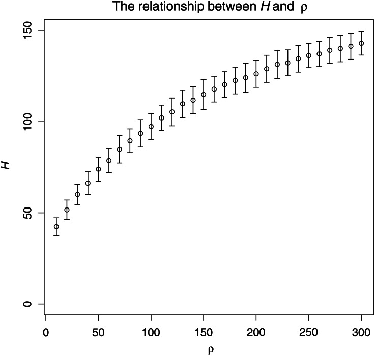
Using boosting, we also found that the number of haplotypes contains the most crucial information on recombination, which agrees with the previous studies (Wall 2000). There is a nonlinear relationship between the number of haplotypes and ρ (Figure 9). However, relatively little information on ρ is contained in H in situations leading to values of H that are very high or very low (i.e., close to its bounds n or 0). According to our experience, the performance of boosting is best, in situations where H tends to be between n/5 and 2n/3. Therefore, when a sliding window analysis is performed, the window size should be adjusted accordingly.

Figure 9.

The relationship between H and ρ. For each ρ (10, 20, …, 300), 200 neutral samples were simulated (n = 200, S = 59). This figure shows the mean and standardized deviation of H computed from the 200 samples of each ρ.

McVean et al. (2002) argue that the rate of recurrent mutation should also be considered when estimating the population recombination rate. In situations where this matters, it would be easy to include recurrent mutations within the boosting framework by using suitable coalescent-based training data. Moreover, the usage of the infinite site model here makes the comparison between boosting and LDhat (slightly) unfair since LDhat permits to model also scenarios more complex than the infinite site model. Note, however, that we do not expect the simulation times for the training scenarios needed with boosting to change much when recurrent mutations are used instead of the infinite-sites model. Thus, this infinite/finite-site issue should not significantly change our conclusions here.

Boosting could be further speeded up in the context of a genome-wide analysis, although it may already be fast enough. Indeed, our analysis suggests that boosting is not very sensitive with respect to the value of S (Figure 6). When conducting a genome-wide scan (using sliding windows), a fixed average value for θ could therefore be used in the training process. This avoids the need for separate training within each window. Alternatively boosting could be pretrained on a grid of values of segregating sites. Such strategies would make the estimation of the recombination rate possible on a normal personal computer, even for whole genomes and large samples.

In the near future, we will provide a free software package on our website (http://www.picb.ac.cn/evolgen/) that implements our approach.

Literature Cited

- Akaike H., 1974. A new look at the statistical model identification. IEEE Trans. Automat. Contr. 19(6): 716–723. [Google Scholar]
- Batorsky R., Kearney M. F., Palmer S. E., Maldarelli F., Rouzine I. M., et al. , 2011. Estimate of effective recombination rate and average selection coefficient for HIV in chronic infection. Proc. Natl. Acad. Sci. USA 108(14): 5661–5666. [DOI] [PMC free article] [PubMed] [Google Scholar]
- Bühlmann P., 2006. Boosting for high-dimensional linear models. Ann. Stat. 34: 559–583. [Google Scholar]
- Bühlmann P., Hothorn T., 2007. Boosting algorithms: regularization, prediction and model fitting. Stat. Sci. 22(4): 477–505. [Google Scholar]
- Chan A. H., Jenkins P. A., Song Y. S., 2012. Genome-wide fine-scale recombination rate variation in Drosophila melanogaster. PLoS Genet. 8(12): e1003090. [DOI] [PMC free article] [PubMed] [Google Scholar]
- Ewing G., Hermisson J., 2010. Msms: a coalescent simulation program including recombination, demographic structure and selection at a single locus. Bioinformatics 26(16): 2064–2065. [DOI] [PMC free article] [PubMed] [Google Scholar]
- Fay J. C., Wu C.-I., 2000. Hitchhiking under positie darwinian selection. Genetics 155: 1405–1413. [DOI] [PMC free article] [PubMed] [Google Scholar]
- Fearnhead P., Donnelly P., 2001. Estimating recombination rates from population genetic data. Genetics 159: 1299–1318. [DOI] [PMC free article] [PubMed] [Google Scholar]
- Fearnhead P., Donnelly P., 2002. Approximate likelihood methods for estimating local recombination rates. J. R. Stat. Soc. Series B Stat. Methodol. 64(4): 657–680. [Google Scholar]
- Fu Y. X., 1997. Statistical tests of neutrality of mutations against population growth, hitchhiking and background selection. Genetics 147: 915–925. [DOI] [PMC free article] [PubMed] [Google Scholar]
- Gusfield D., 1991. Efficient algorithms for inferring evolutionary trees. Networks 21(1): 19–28. [Google Scholar]
- Hey J., 1997. A coalescent estimator of the population recombination rate. Genetics 145: 833–846. [DOI] [PMC free article] [PubMed] [Google Scholar]
- Hill W. G., 1968. Linkage disequilibrium in finite populations. Theor. Appl. Genet. 38: 226–231. [DOI] [PubMed] [Google Scholar]
- Hothorn, T., and P. Bühlmann, 2002 Mboost: model-based boosting, r package version version 0.5–8. Available at: http://cran.r-project.org.
- Hudson R. R., 1985. The sampling distribution of linkage disequilibrium under an infinite allele model without selection. Genetics 109: 611–631. [DOI] [PMC free article] [PubMed] [Google Scholar]
- Hudson R. R., 1987. Estimating the recombination parameter of a finite population model without selection. Genet. Res. 50(3): 245–250. [DOI] [PubMed] [Google Scholar]
- Hudson R. R., 2001. Two-locus sampling distributions and their application. Genetics 159: 1805–1817. [DOI] [PMC free article] [PubMed] [Google Scholar]
- Hudson R. R., 2002. Generating samples under a Wright–Fisher neutral model of genetic variation. Bioinformatics 18(2): 337–338. [DOI] [PubMed] [Google Scholar]
- Hudson R. R., Kaplan N. L., 1985. Statistical properties of the number of recombination events in the history of a sample of DNA sequences. Genetics 111: 147–164. [DOI] [PMC free article] [PubMed] [Google Scholar]
- Kuhner M. K., Yamato J., Felsenstein J., 2000. Maximum likelihood estimation of recombination rates from population data. Genetics 156: 1393–1401. [DOI] [PMC free article] [PubMed] [Google Scholar]
- Li N., Stephens M., 2003. Modeling linkage disequilibrium and identifying recombination hotspots using single-nucleotide polymorphism data. Genetics 165: 2213–2233. [DOI] [PMC free article] [PubMed] [Google Scholar]
- Lin K., Li H., Schlöttterer C., Futschik A., 2011. Distinguishing positive selection from neutral evolution: boosting the performance of summary statistics. Genetics 187: 229–244. [DOI] [PMC free article] [PubMed] [Google Scholar]
- McVean G., Awadalla P., Fearnhead P., 2002. A coalescent-based method for detecting and estimating recombination from gene sequences. Genetics 160: 1231–1241. [DOI] [PMC free article] [PubMed] [Google Scholar]
- Myers S. R., Griffiths R. C., 2003. Bounds on the minimum number of recombination events in a sample history. Genetics 163: 375–394. [DOI] [PMC free article] [PubMed] [Google Scholar]
- Pritchard J. K., Przeworski M., 2001. Linkage disequilibrium in humans: models and data. Am. J. Hum. Genet. 69(1): 1–14. [DOI] [PMC free article] [PubMed] [Google Scholar]
- Reed F. A., Tishkoff S. A., 2006. Positive selection can create false hotspots of recombination. Genetics 172: 2011–2014. [DOI] [PMC free article] [PubMed] [Google Scholar]
- Sabeti P. C., Reich D. E., Higgins J. M., Levine H. Z., Richter D. J., et al. , 2002. Detecting recent positive selection in the human genome from haplotype structure. Nature 419(6909): 832–837. [DOI] [PubMed] [Google Scholar]
- Sabeti P. C., Schaffner S. F., Fry B., Lohmueller J., Varilly P., et al. , 2006. Positive natural selection in the human lineage. Science 312(5780): 1614–1620. [DOI] [PubMed] [Google Scholar]
- Sved J. A., 1968. The stability of linked systems of loci with a small population size. Genetics 59: 543–563. [DOI] [PMC free article] [PubMed] [Google Scholar]
- Tajima F., 1989. Statistical method for testing the neutral mutation hypothesis by DNA polymorphism. Genetics 123: 589–595. [DOI] [PMC free article] [PubMed] [Google Scholar]
- Wakeley J., 1997. Using the variance of pairwise differences to estimate the recombination rate. Genet. Res. 69(1): 45–48. [DOI] [PubMed] [Google Scholar]
- Wall J. D., 2000. A comparison of estimators of the population recombination rate. Mol. Biol. Evol. 17(1): 156–163. [DOI] [PubMed] [Google Scholar]
- Wall J. D., 2004. Estimating recombination rates using three-site likelihoods. Genetics 167: 1461–1473. [DOI] [PMC free article] [PubMed] [Google Scholar]
- Wiuf C., 2002. On the minimum number of topologies explaining a sample of DNA sequences. Theor. Popul. Biol. 62(4): 357–363. [DOI] [PubMed] [Google Scholar]
Associated Data
This section collects any data citations, data availability statements, or supplementary materials included in this article.