Continuum-kinetic-microscopic model of lung clearance due to core-annular fluid entrainment

Abstract

The human lung is protected against aspirated infectious and toxic agents by a thin liquid layer lining the interior of the airways. This airway surface liquid is a bilayer composed of a viscoelastic mucus layer supported by a fluid film known as the periciliary liquid. The viscoelastic behavior of the mucus layer is principally due to long-chain polymers known as mucins. The airway surface liquid is cleared from the lung by ciliary transport, surface tension gradients, and airflow shear forces. This work presents a multiscale model of the effect of airflow shear forces, as exerted by tidal breathing and cough, upon clearance. The composition of the mucus layer is complex and variable in time. To avoid the restrictions imposed by adopting a viscoelastic flow model of limited validity, a multiscale computational model is introduced in which the continuum-level properties of the airway surface liquid are determined by microscopic simulation of long-chain polymers. A bridge between microscopic and continuum levels is constructed through a kinetic-level probability density function describing polymer chain configurations. The overall multiscale framework is especially suited to biological problems due to the flexibility afforded in specifying microscopic constituents, and examining the effects of various constituents upon overall mucus transport at the continuum scale.

1 Introduction

Millions of bacteria spores, toxic and inert particles, and pollen seeds are aspirated into the human lung in the course of a day. Remarkably, the lung airways are sterile in healthy individuals [30] with most of the inhaled pathogens cleared from the lung by a mechanical process in which mucus entraps aspirated particles and is then itself evacuated from the lung by the action of numerous cilia lining the lung bronchi [21], in conjunction perhaps with clearance induced by gradients in the surface tension of the airway liquid [14]. Upon breakdown of this healthy-state mucociliary transport mechanism, cough can clear mucus from the lung due to the action of shear and pressure forces upon the airway surface liquid. One model of this process is to consider a core-annular flow in an airway with the rapidly accelerating air core setting the surrounding airway surface liquid in motion. Even this simplified model, which neglects formation of airway-blocking plugs of fluid, exhibits significant complexity associated with flow-instability dynamics and the viscoelastic nature of the airway surface liquid.

Work by Clarke et al. [13] showed that the dynamics of wave formation on the annular liquid layer by the core air flow are important and lead to flow resistance much larger than would be expected from viscosity in a perfectly cylindrical flow (Fig 1). King et al. [29] investigated differences between laminar and turbulent flow as well as the effects of oscillatory flow as would be encountered in the lung during breathing. Markedly different responses of the flow, as measured by overall flow resistance, were observed for different viscoelastic bulk moduli of the annular fluid. Experimental studies of air propeling a surrounding Newtonian or viscoelastic fluid vertically against gravity have also been carried out by Kim [28], [27], showing that upward transport can occur once the annular fluid reaches a critical thickness. Scherer and Burtz [44] showed that the waves induced in a Newtonian annular fluid layer grow and eventually break up into droplets that are entrained by the airflow and expelled. The wide variety of interactions between the core flow and surrounding annular liquid is documented in the review by Joseph [23].

Fig. 1.

Waves induced in an annular liquid layer by core air flow at low, 30 l/m (top) and high, 60 l/m (bottom) volume flow rates in a vertical tube of 1 cm diameter. At the low flow rate ripples form on the surface accumulating into an advancing front that transports mass. At the high flow rate irregular waves are observed. (Photographs courtesy of Jeffrey Oleander, Roberto Camassa, UNC Joint Applied Mathematics & Marine Science Fluids Lab)

Theoretical work on the core-annular transport mechanism includes the study by Blake [5] in which qualitative flow behavior was discussed using a Poiseuille flow approximation. A series of linear flow stability studies were carried out by Bai, Chen and Joseph [2], [11], followed by later numerical studies of nonlinear behavior [1]. An overview of various approaches has been compiled by Grotberg [17]. More recent work includes direct numerical simulation of the biphasic flow using Lagrangian tracking of the interface by Li & Renardy [34], the level-set approach of Kang et al [25], and volume-of-fluid methods [45]. Most of the published studies assume Newtonian fluid behavior or adopt some known viscoelastic model hypothesized to accurately capture non-Newtonian effects.

Computational modeling of core-annular flows in lung bronchi is challenging due to the complex viscoelastic behavior of mucus. By weight fractions, mucus in healthy individuals contains approximately 95% water, 1% salts, 1% free proteins, and 1% glycoproteins known as “mucins” [21]. Lipids and deoxyribonucleic acid (DNA) may also be present. Mucus behaves like a viscoelastic gel, principally due to the cross-linked mucin glycoproteins. In pathological states the concentration of mucins can increase to as much as 8%, completely stopping normal mucociliary clearance and also rendering clearance by cough difficult. One of the prime objectives in computational modeling of lung clearance is to be able to link chemical composition of mucus to overall mechanical behavior with the goal of identifying drugs whose effect would aid in efficient evacuation of mucus from bronchi. Mucus exhibits complex rheological behavior both in bulk and at the microscale [32], and relatively small concentrations of non-mucin components can significantly affect the viscoelastic response [39].

There is no known, universally-valid, constitutive law that captures mucus mechanical behavior over all flow regimes encountered in the lung. Essentially, this is due to the significant microscopic changes in configuration that occur in response to changes in macroscopic flow conditions. Common continuum-level viscoelastic models can capture only some limited aspect of the microscopic configurational changes. For example, the widely used FENE-P model [43] can model stretching of well-separated polymer chains in response to background shear flow, but cannot account for cross-links between chains. An alternative to the extremely difficult task of establishing a constitutive law for mucus is to devise a multiscale computational procedure that directly links microsopic and macroscopic behavior. In particular, it is of considerable interest to construct an algorithm that can capture complicated microscopic behavior, not only the dynamics of mucus at high mucin concentration, but also changes induced by pharmaceuticals.

This paper introduces a multiscale model of how central air flow induces peripheral mucus transport in a tube-like geometry. Three different levels of description of the process are used:

1. A microscopic level defined here as the stochastic process of mucin conformational changes in response to mean flow conditions, and modeled by stochastic differential equations (7);

2. A kinetic level which tracks the time evolution of probability density functions that capture some aspect of the flow. Newtonian behavior of the core air flow and the solvent component of the mucus is modeled by Boltzmann equations (10–11). Polymer cross-link and conformational changes are modeled by Fokker-Planck equations (12–13), and passive transport is described by an advection (14) equation;

3. A continuum level which follows overall mass and momentum transport in the coannular flow as described by bulk, cross-section averaged equations in airway segments (58–60) and at airway junctions (64–66).

The microscopic and kinetic levels compute the local, instantaneous behavior of mucus components in the background flow provided by the continuum level. The continuum level furnishes a computationally tractable model to advance the overall system in time in response to far-field boundary conditions (e.g. the respiratory cycle). Two-way coupling exists between each level as detailed in Sect. 5. In brief, the microscopic chemical composition and polymer chain configuration data are advected by the continuum flow. A new microscopic configuration is obtained as the system relaxes locally in response to changes induced by the flow. The new microscopic configuration is used to reconstruct interfaces and determine mechanical stress transfer to the macroscale continuum medium, information needed to subsequently advance the flow by a time step.

2 Microscopic model

Core-annular flow in an airway involves a complex mixture of air, mucus, aspirated particles and droplets. The purpose of this paper is to introduce a methodology of linking microscopic properties to overall continuum transport, and microscopic modeling will focus on mucus, the most complex constituent. After a review of mucus properties, a simplified model is adopted in which the mucus gel-formation process is captured through transition rates for cross-links formed by mucins.

2.1 Mucus properties

Mucus is a dilute aqueous solution of various proteins, salts and mucins. Mucins are polymeric compounds with a high molecular mass, on the order of 10⁶ atomic mass units. The typical structure of a mucin (Fig. 2) consists of a long polypeptide central chain from which numerous polysccharide side chains extend imparting an overall brush geometry. Hydrophobic patches are found at intervals along the central chain. A key physiological property of mucins is their propensity to form gels [3]. The detailed mechanism by which gel formation occurs is unknown and is a formidable problem in molecular biophysics given that mucins are the largest glycoprotein macromolecules in the body [26]. Plausible mechanisms include:

Fig. 2.

Schematic of complex, polymeric structure of a typical mucin

1. polymer entanglement [10];

2. cross-linkage between chains by non-covalent bonds [3];

3. hydrophobic interactions between chains [8];

4. carbohydrate-carbohydrate interactions between mucins [37].

Given the variety of plausible microscopic interaction mechanisms it is not surprising that the rheology of mucus is complex, highly dependent on constituent concentrations and applied forces (Fig. 4 from [32] shows variation in viscosity over four orders of magnitude from 10⁻² to 10² Pa).

Fig. 4.

Lattice sites, continuum control volumes and directions D of D2Q9 lattice Boltzmann model.

2.2 Mucin transient network model

In order to make any progress in the understanding of overall mucus rheological properties simplified models that capture relevant microscopic degrees of freedom, while neglecting the vast majority of the details of the molecular interactions, are needed. The focus in this paper will be on capturing cross-link formation. Polymers that tend to form cross-links between chains are said to be associative [49], [15], [16] and a large body of transient network theory [47] has been developed that describes to various levels of detail the dynamic process of cross-linkage formation. From this large body of literature on transient networks, a simple Brownian dynamics model [48], [12] is adopted here to exemplify how a multiscale computational procedure can link macroscale transport to microscale network properties.

Mucins are considered to form cross-linkages only at their end-segments (telechelic chains). This corresponds to polymers of structure A-B-A with B a long water-soluble polymer and A a short hydrophobic segment. Such structures are known to form closed-loop micelles and at high concentrations linkages can form between adjacent micelles. Vaccaro and Marrucci [48] introduced a simple model in which the network in built from only two types of elements: (1) active chains between network nodes, and (2) pendent or dangling chains detached from the network at one end (Fig. 3).

Fig. 3.

Schematic of overall mucus-air model. Cross-linkages are formed between micelles arising from mucins modeled as telechelic chains. Hydrophobic ends denoted by red disks, water-soluble middle segment denoted by a line. Force in the network is preponderently carried by the cross-links (thick, green lines). Some of the chains form closed loops onto the same network node and do not carry any appreciable network load. Other chains have a dangling free end that potentially can form additional cross linkages. The friction coefficient of the solvent with free nodes at the end of a dangling chain is ζ_free, that with the larger micelle nodes is ζ_node, ζ_node > ζ_free. The mucins are surrounded by water solvent molecules (blue disks). The mucus layer forms an interface with an adjacent air region (black circles).

The major simplification of this model is that the precise network topology is not considered. Rather, the dynamics are reduced to tracking n_a, the number of active segments forming a cross-link, and n_d, the number of dangling segments which potentially could form a cross-link. The influence of loops is not included in the model. The configuration of polymer i is reduced to the single end-to-end or dumbbell vector r_i which has length r_i ≡ ||r_i||. The polymer configuration changes in response to:

1. overall mean flow conditions specified by a local value κ of the velocity gradient tensor

   $$\mathit{\kappa }=\nabla \mathit{u},{\kappa }_{i,j}=\frac{\partial u_i}{\partial x_j},$$ (1)

   with u the continuum-level fluid velocity;

2. entropic spring forces in the dumbbell as given by the FENE-P law

   $$\mathit{F}(\mathit{r})=\frac{H\mathit{r}}{1-{\mathit{r}}^2/r_{max}^2},$$ (2)

   with r_max the maximum allowed elongation of a dumbbell;

3. Brownian forcing due to the solvent.

Let τ denote the lifetime of a node in the network and α the association rate of dangling segments. Both of these quantities depend on the length of an end-to-end vector. More highly stretched links have shorter lifetimes τ. Highly stretched dangling chains have large α values since they explore larger regions of space in which to form a new active link. The length-dependence of the node lifetime and association rate shall be assumed isotropic, τ (r), α (r), with τ′(r) < 0, α′ (r) > 0. The probability that an active segment becomes a dangling one in time interval δt due to dissociation of either of its ends is

$$P_{\text{dissoc}}=1-exp\left[-\frac{2\delta t}{\tau (r)}\right].$$ (3)

The node lifetime is determined by the details of the chemical bond of a dangling end to become part of a micelle. For a simple parabolic energy model of the link characterized by a width of the bond energy barrier d, and depth U₀, the node lifetime dependence on the length of an active segment r_a can be given as [12]

$$\tau (r)={\tau }_{0}exp\left[-\frac{H^2{d}^2{r}^2}{4U_0{k}_{B}T{(1-r^2/r_{max}^2)}^2}\right].$$ (4)

The linear association probability model of [12] is

$$P_{\text{assoc}}=1-exp[-\alpha (r)\delta t],$$ (5)

$$\alpha (r)={\alpha }_0+\frac{{\alpha }_{1}r}{1-r^2/r_{max}^2}.$$ (6)

The time evolution of an end-to-end vector is given by a stochastic differential equation given here as the discretization resulting from a first-order explicit scheme

$$\mathit{r}(t+\delta t)=\mathit{r}(t)+\mathit{\kappa }·\mathit{r}\delta t-(H/\zeta )\mathit{F}(\mathit{r})\delta t+\sqrt{2k_{B}T/\zeta }\delta \mathit{w}(t),$$ (7)

in a control volume small enough such that variations of r with respect to x, and associated macroscale advection effects are negligible, U (t, x) · ∇_xr (x) ≅ = 0. The ends of the dumbbell specified by r interact with the surrounding fluid either as free nodes with friction coefficient ζ_free or as part of a micelle with friction coefficient ζ_node. The average friction coefficient coefficient felt by a dumbbell is given by the harmonic average ζ = ζ₁ζ₂/(ζ₁ + ζ₂), with

$${\zeta }_a=\frac{{\zeta }_{\text{node}}}{2},{\zeta }_d=\frac{{\zeta }_{\text{free}}{\zeta }_{\text{node}}}{{\zeta }_{\text{free}}+{\zeta }_{\text{node}}},$$ (8)

for active and dangling segments, respectively. The stochastic term δw (t) in (7) is the discretization of a Wiener process with zero mean and variance δt.

2.3 Microscopic expression of continuum stress

The conformation and linkages within the chains lead to an overall macroscopic stress T which is computed using Kramers-Kirkwood expression [4]. For the reversible network model from 2.2 the stress is obtained as an average over the dangling and active dumbbells in some control volume

$$\mathit{T}={\langle {\mathit{r}}_a\mathit{F}({\mathit{r}}_a)\rangle }_a+{\langle {\mathit{r}}_d\mathit{F}({\mathit{r}}_d)\rangle }_d.$$ (9)

3 Kinetic models

In principle, direct numerical simulation of the stochastic differential equations (7) and averaging over configurations (9) could furnish the additional viscoelastic stress that expresses momentum transfer between a continuum macroscale and the microscopic transient network. However, the computational effort needed to reduce the sampling noise is prohibitive [42], even after application of variance reduction ideas [6], [31], [24]. This paper uses an intermediate kinetic level of description as a bridge between the microscopic model of Section 2 and a bulk transport model to be presented in Section 4. The kinetic level consists of evolution equations for probability density functions (PDFs) for various components of the airway surface liquid. Lattice based techniques are introduced for efficient computational simulation.

3.1 Fluid Boltzmann equations

Kinetic models are introduced for the core airflow and Newtonian solvent within mucus. Let f_g (t, x, v) be the PDF of finding a gas particle with mass m_g with velocity v at position x and time t. The time evolution is given by the Boltzmann equation

$$\frac{\partial f_g}{\partial t}+\mathit{v}·\frac{\partial f_g}{\partial \mathit{x}}=I_c(f_g),$$ (10)

with I_c (f_g) the Boltzmann collision integral [46]. A similar equation governs the time evolution of the mucus solvent PDF f_s (t, x, v)

$$\frac{\partial f_s}{\partial t}+\mathit{v}·\frac{\partial f_s}{\partial \mathit{x}}+\frac{\mathit{P}}{m_s}·\frac{\partial f_s}{\partial \mathit{v}}=I_c(f_s),$$ (11)

with P the force exerted on the solvent by mucin polymers within the transient network.

3.2 Transient network Fokker-Planck equations

Let f_a (t, x, r), f_d (t, x, r) denote the PDFs for active, dangling links to have end-to-end vector r at position x and time t. The time evolution of these PDFs is given by the Fokker-Planck equations

$$\frac{\partial f_a}{\partial t}+\mathit{u}·\frac{\partial f_a}{\partial \mathit{x}}+\frac{\partial }{\partial \mathit{r}}·\left[\left(\mathit{\kappa }·\mathit{r}-\frac{1}{{\zeta }_a}\mathit{F}(\mathit{r})-D_a\frac{\partial }{\partial \mathit{r}}\right)f_a\right]=S(f_a,f_d),$$ (12)

$$\frac{\partial f_d}{\partial t}+\mathit{u}·\frac{\partial f_d}{\partial \mathit{x}}+\frac{\partial }{\partial \mathit{r}}·\left[\left(\mathit{\kappa }·\mathit{r}-\frac{1}{{\zeta }_d}\mathit{F}(\mathit{r})-D_d\frac{\partial }{\partial \mathit{r}}\right)f_d\right]=-S(f_a,f_d),$$ (13)

with diffusion coefficients D_a = k_BT/ζ_a, D_d = k_BT/ζ_d, and source term

$$S(f_a,f_d)=\alpha (r)f_d-\frac{2f_a}{\tau (r)},$$ (14)

capturing transitions between active and dangling link states. The mucins within closed loops or freely floating in the solvent have a passive role: the contribute to inertia, but exchange negligible momentum with the overall flow. Let f_p (t, x) denote the PDF of the closed loop and free mucins with evolution equation

$$\frac{\partial f_p}{\partial t}+\mathit{u}·\frac{\partial f_p}{\partial \mathit{x}}=0.$$ (15)

All mucins (active, dangling, loops, free chains) are assumed to be advected by a flowfield u defined on a control volume around each point x. Note that the hypothesis of constant number of active and dangling mucins, n_a + n_d = constant, can readily be extended to include transitions to loop and free states by including appropriate source terms in (12–15).

3.3 Lattice discretization

Solving the Boltzmann equations (10–11) and Fokker-Planck system (12–14) is a difficult computational problem due to the dependence of the PDFs on seven independent variables: (t, x, r) for f_a, f_d, and (t, x, v) for f_g, f_s. A computationally tractable method is the lattice Boltzmann approach [46], [40] in which the functional dependence of the PDFs f_g, f_s, on the continuum of possible velocities vectors v, f_g (t, x, v), f_s (t, x, v), is reduced to a discrete set f_g,l (t, x) = f_g (t, x, e_l), f_s,l (t, x) = f_s (t, x, e_l), for some choice of a set of directions D = {e₀, e₁, …, e_n}. Typically, the directions e_l, l =0, …, n are chosen as translation vectors between nodes x_I on a regular lattice L = {x_I, I = 0, 1, …, N } with some desired symmetry properties. A widely used set of directions is the so-called D2Q9 model in two dimensions L = {(0, 0), (±1, 0), (0, ±1), (±1, ±1)} (Fig. 4). An analagous set of directions for three dimensions is the D3Q19 lattice [46]. Likewise, the dependence of f_a, f_d on the continuum of possible dumbbell vectors r can be reduced to a discrete set f_a,l (t, x) = f_a (t, x, e_l), f_d,l (t, x) = f_d (t, x, e_l), l = 0, …, n. The specifics of a lattice approach depend on the kinetic equation, and are considered separately for the Boltzmann and Fokker-Planck equations. The two-dimensional case is presented – extensions to three dimensions are straightforward.

3.3.1 Fluid lattice Boltzmann model

Consider a two-dimensional domain with lattice sites x_I = ie_x + je_y, I ≡ i + n_yj), 0 ≤ i ≤ n_x, 0 ≤ j ≤ n_y (Fig. 4). Let γ denote an element in the set of species Γ = {p, a, d, s, g} (passive mucins, active links, dangling segments, solvent, gas), and let Γ′= {s, g} denote the species for which we define velocity PDFs. A standard immiscible, two-color lattice Boltzmann model [19], [18] is used for solvent and air. The force imbalance between solvent and air particles at the mucus-air interface is the surface tension.

In the lattice Boltzmann method the time evolution of the distribution functions f_γ,l is determined by two operations:

1. A streaming step

   $${\overline{f}}_{\gamma ,l}(t+\mathrm{\Delta }t,\mathit{x})=f_{\gamma ,l}(t,\mathit{x}-{\mathit{e}}_l\mathrm{\Delta }t),$$ (16)

   in which the PDF for each lattice direction is advected;

2. A relaxation step that models particle collisions. The complicated Boltzmann collision integral is replaced by a single time scale relaxation

   $$f_{\gamma ,l}(t+\mathrm{\Delta }t,\mathit{x})=F_{\gamma ,l}-\frac{1}{{\tau }_{\gamma }}\left[{\overline{f}}_{\gamma ,l}(t+\mathrm{\Delta }t,\mathit{x})-f_{\gamma ,l}^{\text{eq}}(t+\mathrm{\Delta }t,\mathit{x})\right],$$ (17)
   towards the Maxwell-Boltzmann equilibrium distributions

   $$f_{\gamma .l}^{\text{eq}}(t+\mathrm{\Delta }t,\mathit{x})={\rho }_{\gamma }{w}_l\left[1+\frac{{\mathit{e}}_l·\mathit{u}}{c_s^2}+\frac{{({\mathit{e}}_l·\mathit{u})}^2}{2c_s^2}-\frac{{\mathit{u}}^2}{2c_s^2}\right],$$ (18)
   for each species γ ∈ {g, s} with characteristic relaxation time τ_γ, density of species with molecular mass m_γ

   $${\rho }_{\gamma }=m_{\gamma }\sum _{l=0}^n{f}_{\gamma ,l},$$ (19)

   sound speed c_s, and weights w_l (see, e.g., [46]). This is known as the Bhatnagar-Gross-Krook (BGK) approximation. The F_γ,l term captures effects of external forces, and is used here to include surface tension effects at phase interfaces.

The {p, a, d} species are assumed to be passively transported and simply add to the overall inertia. At each lattice site I, a mass and momentum density are defined by

$${\mathit{q}}_I={\left(\rho \rho \mathit{u}\right)}_I,$$ (20)

and a bulk density ρ, and bulk velocity u is defined by

$$\rho =\sum _{\gamma \in \mathrm{\Gamma }}{m}_{\gamma }\sum _{l=0}^n{f}_{\gamma ,l},{\rho }^{\prime }=\sum _{\gamma \in {\mathrm{\Gamma }}^{\prime }}{m}_{\gamma }\sum _{l=0}^n{f}_{\gamma ,l},$$ (21)

$$\rho \mathit{u}=\frac{\rho }{{\rho }^{\prime }}\sum _{\gamma \in {\mathrm{\Gamma }}^{\prime }}{m}_{\gamma }\sum _{l=0}^n{f}_{\gamma ,l}{\mathit{e}}_l,$$ (22)

with m_γ the molecular mass of species γ.

Relations (21–22) define the advection velocity in (12–13). Note that the advection velocity is of the form

$$\mathit{u}=\sum _{l=1}^n{c}_l{\mathit{e}}_l,$$ (23)

with

$$c_l=\frac{{\sum }_{\gamma \in {\mathrm{\Gamma }}^{\prime }}{m}_{\gamma }{f}_{\gamma ,l}}{{\sum }_{l=0}^n{\sum }_{\gamma \in {\mathrm{\Gamma }}^{\prime }}{m}_{\gamma }{f}_{\gamma ,l}},\sum _{l=0}^n{c}_l=1,c_l\ge 0,$$ (24)

and $\left|\right|{\mathit{e}}_i\left|\right|\le \sqrt{N_d}$, with N_d the number of space dimensions, hence $\left|\right|\mathit{u}\left|\right|\le \sqrt{N_d}$.

The continuum surface force approach [7] is used to capture surface tension effects at sites that contain the gas-solvent interface as outlined by Lishchuk, Care & Halliday [35]. At lattice sites containing both gas and solvent (air and water), a density difference is defined as ρ_g−s(t, x) = ρ_g(t, x) − ρ_s(t, x), with ρ_g, ρ_s defined by (19), as well as a joint density ρ_g+s(t, x) = ρ_g(t, x) + ρ_s(t, x). Surface tension effects are included through the term

$$F_l=\frac{\sigma }{2c_s^{2}R}{\mathit{e}}_l·\nabla \left(\frac{{\rho }_{g-s}(t,\mathit{x})}{{\rho }_{g+s}(t,\mathit{x})}\right),$$ (25)

included in the relaxation step (17) through F_g,l = F_l, F_s,l = − F_l. In (25), σ is the surface tension coefficient and R is the local radius of curvature determined by

$$R^{-1}=[(\mathit{nn}-\mathit{I})·\nabla ]·\mathit{n},$$ (26)

with the surface normal determined as n = ∇ρ_g−s/||∇ρ_g−s||, evaluated by second-order centered finite differencing.

3.3.2 Polymer lattice Fokker-Planck model

The Fokker-Planck equations for the transient mucin network (12–15) describe advection by the velocity field u, straining of the network by the velocity gradient κ, relaxation by mucin forces F (r) and thermal motions D_γ∂f_γ/∂r, and source terms S (f_a, f_d). An operator splitting approach is adopted in which in a first stage the advection and source terms are considered

$$\frac{\partial f_a}{\partial t}+\mathit{u}·\frac{\partial f_a}{\partial \mathit{x}}=S(f_a,f_d),$$ (27)

$$\frac{\partial f_d}{\partial t}+\mathit{u}·\frac{\partial f_d}{\partial \mathit{x}}=-S(f_a,f_d),$$ (28)

$$\frac{\partial f_p}{\partial t}+\mathit{u}·\frac{\partial f_p}{\partial \mathit{x}}=0.$$ (29)

The effects in the first stage of the splitting are captured by the streaming step

$${\overline{f}}_{\gamma ,l}(t+\mathrm{\Delta }t,\mathit{x})=\sum _{l=0}^n{c}_l[f_{\gamma ,l}(t,\mathit{x}-{\mathit{e}}_l\mathrm{\Delta }t)+S_{\gamma }\mathrm{\Delta }t],$$ (30)

for γ ∈ {a, d, p}, and with coefficients c_l from (24), and S_γ equal to (S, − S, 0) for γ = a, d, p respectively. This is simply the update given by marching along the characteristics of the advection operator ∂/∂t + u · ∂/∂x, taking into account source terms.

The more difficult aspect in the lattice modeling of the Fokker-Planck equation is the second stage of the splitting

$$\frac{\partial f_a}{\partial t}+\frac{\partial }{\partial \mathit{r}}·\left[\left(\mathit{\kappa }·\mathit{r}-\frac{1}{{\zeta }_a}\mathit{F}(\mathit{r})-D_a\frac{\partial }{\partial \mathit{r}}\right)f_a\right]=0,$$ (31)

$$\frac{\partial f_d}{\partial t}+\frac{\partial }{\partial \mathit{r}}·\left[\left(\mathit{\kappa }·\mathit{r}-\frac{1}{{\zeta }_d}\mathit{F}(\mathit{r})-D_d\frac{\partial }{\partial \mathit{r}}\right)f_d\right]=0,$$ (32)

intended to capture the effect of the relaxation terms that lead to viscoelastic behavior. Various approaches have been proposed to model viscoelastic effects in a lattice Boltzmann method. Onishi, Chen & Ohashi [41] maintain the idea of a BGK relaxation with a single characteristic relaxation time, but use a modified equilibrium distribution to mimic viscoelastic effects. Malaspinas, Fietier & Deville [36] have recently proposed a lattice method for both the momentum transport equation as well as the transport equation for the configuration tensor in an Oldroyd-B or FENE-P model. While these approaches do exhibit viscoelastic effects, they in effect impose a continuum-level constitutive law, which is known not to be fully accurate, upon the kinetic formulation. A more appealing alternative is not to seek to mimic some a priori specified continuum constitutive model (e.g. Oldroyd-B or FENE-P), but rather to introduce a correct description of kinetic-level relaxation effects which lead to viscoelasticity.

Here, a novel lattice relaxation operator is introduced that in contrast to the BGK procedure (17) or single relaxation FENE-type models is capable of capturing all time scales of the polymer gel. In brief, this reformulation is based upon a variational description of solutions to Fokker-Planck equations [22] of the form

$$\frac{\partial f}{\partial t}=\frac{\partial }{\partial \mathit{r}}·\left[\frac{\partial \mathrm{\Phi }}{\partial \mathit{r}}f\right]+\frac{1}{\beta }\frac{\partial }{\partial \mathit{r}}·\frac{\partial f}{\partial \mathit{r}},$$ (33)

in which Φ is a potential function, in this case

$$\mathrm{\Phi }(\mathit{r})=-\frac{1}{2}{\mathit{r}}^T\mathit{\kappa }\mathit{r}+\frac{H}{2\zeta }log\left(1-\frac{{\mathit{r}}^2}{r_{max}^2}\right),$$ (34)

with 1/β = D. If f^(k−1) is the solution of (33) at time t^(k−1), the solution at the next time step f^(k) can be obtained from minimizing the functional

$$\mathcal{L}(g)=\frac{1}{2}d{\left(f^{(k-1)},g\right)}^2+\mathrm{\Delta }t\mathcal{G}(g),$$ (35)

stated as f^(k) = argmin_g (g), with (g) the free energy functional

$$\mathcal{G}(g)=\mathcal{E}(g)+{\beta }^{-1}\mathcal{S}(g),$$ (36)

$$\mathcal{E}(g)={\int }_{{\mathbb{R}}^{N_d}}\mathrm{\Phi }(\mathit{r})g(\mathit{r})\text{d}\mathit{r},\mathcal{S}(g)={\int }_{{\mathbb{R}}^{N}d}g(\mathit{r})logg(\mathit{r})\text{d}\mathit{r},$$ (37)

and d (f, g) the Wasserstein distance of order two between probability densities f, g

$$d{(f,g)}^2=\underset{p\in \mathrm{\Gamma }(f,g)}{inf}{\int }_{{\mathbb{R}}^{N_d}\times {\mathbb{R}}^{N_d}}{\left|\right|x-y\left|\right|}_2^2\text{d}p(x,y),$$ (38)

with Γ the set of all joint measures with marginals f, g. The Wasserstein distance can also be expressed as

$$d{(f,g)}^2=inf\left(\mathbb{E}\left[{\left|\right|X-Y\left|\right|}_2^2\right]\right),$$ (39)

with the infinum taken over all random variables X, Y with laws f, g respectively, providing an interpretation of the Wasserstein distance between PDFs as the minimum second moment difference expectation. This result by Jordan, Kinderlehrer & Otto [22] states that the solution to the Fokker-Planck equation follows the steepest descent direction of the (f) functional with respect to the Wasserstein metric.

In the context of lattice methods, this variational characterization allows definition of a simplified relaxation operator, much as the Bhatnagar-Gross-Krook operator (17) is a simplification of the collision integral in the Boltzmann equation. At the end of the streaming stage (30), the set of PDFs f̄_l (t + Δt, x) = f̄(t + Δt, x, e_l) is defined at each lattice site x for active and dangling mucin links (the a, d mucin indices are temporarily suppressed for clarity). From the f̄_l PDFs along each direction e_l of the lattice, a reconstruction h of the overall PDF can be obtained

$$h(t+\mathrm{\Delta }t,\mathit{x},\mathit{r})=\mathcal{R}\left(\left\{{\overline{f}}_l(t+\mathrm{\Delta }t,\mathit{x}),l=0,\dots ,n\right\}\right).$$

We take the PDF obtained by reconstruction of the directional PDFs from the streaming stage as an initial condition for the second stage of the operator splitting procedure. The JKO result states that at each lattice site x, f (t + δt, x, r) the solution for (33) is

$$f(t+\mathrm{\Delta }t,\mathit{x},\mathit{r})=arg\underset{g(\mathit{r})}{min}\left[\frac{1}{2}d(h(t+\mathrm{\Delta }t,\mathit{x},\mathit{r}),g)+\mathrm{\Delta }t\mathcal{G}(g)\right],$$ (40)

an operation formally denoted as

$$f(t+\mathrm{\Delta }t,\mathit{x},\mathit{r})=\mathcal{F}(h(t+\mathrm{\Delta }t,\mathit{x},\mathit{r})).$$ (41)

The solution from solving the variational problem (40) is used to define new directional PDFs by an averaging operation

$$f_l(t+\mathrm{\Delta }t,\mathit{x})=\mathcal{A}(f(t+\mathrm{\Delta }t,\mathit{x},\mathit{r})).$$ (42)

The overall procedure is a reconstruct, flow in gradient direction, average algorithm reminiscent of reconstruct-evolve-average, Riemann-based methods for hyperbolic conservation laws [33]. Various , , operators may be used. Here, a simple collocation approach is adopted with identity reconstruction and averaging operators, maintaining the discrete direction approach of a lattice method, in which the approximation

$$f(t,\mathit{x},\mathit{r})=\sum _{l=0}^n{f}_l(t,\mathit{x})\delta (\mathit{r}-{\mathit{e}}_l),$$ (43)

is used for a PDF. In (43), δ (r − e_l) is the Dirac-delta distribution associated with end-to-end vectors in the direction e_l.

A discretely-supported representation of the PDFs allows considerable simplification in the computation of the Wasserstein distance detween PDFs g, h (38). The marginality conditions on the the measure p in (38) are

$${\int }_{A\times {\mathbb{R}}^{N_d}}\text{d}p(x,y)={\int }_{A}g(x)\text{d}x,{\int }_{{\mathbb{R}}^{N_d}\times B}\text{d}p(x,y)={\int }_{B}h(y)\text{d}y,$$ (44)

for any subsets A, B ⊂ ℝ^N_d. The discretely supported PDF representations are

$$g(t,\mathit{x},\mathit{r})=\sum _{l=0}^n{g}_l(t,\mathit{x})\delta (\mathit{r}-{\mathit{e}}_l),h(t,\mathit{x},\mathit{r})=\sum _{l=0}^n{h}_l(t,\mathit{x})\delta (\mathit{r}-{\mathit{e}}_l),$$ (45)

with normalization conditions

$$\sum _{l=0}^n{g}_l(t,\mathit{x})=\sum _{l=0}^n{h}_l(t,\mathit{x})={\rho }_M(t,\mathit{x}).$$ (46)

The overall density of mucin links at a lattice site, ρ_M (t, x), is assumed not to change during the relaxation stage. For discretely supported PDFs g, h, the joint PDF can be represented by a (n + 1) × (n + 1) matrix A = [A_ij] that satisfies the marginality conditions

$$\sum _{j=0}^n{A}_{ij}=g_i,i=0,1,\dots ,n,\sum _{i=0}^n{A}_{ij}=h_j,j=0,1,\dots ,n.$$ (47)

The Wasserstein distance is now expressed as discrete, linear optimization problem

$$d_{\mathit{A}}{(g,h)}^2=\underset{\mathit{A}}{min}\sum _{i,j=0}^n{A}_{ij}{c}_{ij}^2,$$ (48)

with constraints (44) and costs

$$c_{ij}^2={\left|\right|{\mathit{e}}_i-{\mathit{e}}_j\left|\right|}_2^2.$$ (49)

For a discretely supported PDF g, the free energy functional (g) becomes

$${\mathcal{G}}_{\mathit{A}}(g)=\sum _{l=0}^n\left(\mathrm{\Phi }({\mathit{e}}_l)+{\beta }^{-1}log{g}_l\right)g_l,$$ (50)

leading to an expression for the overall functional (35)

$${\mathcal{L}}_{\mathit{A}}(g;h)-\frac{1}{2}{d}_{\mathit{A}}{(g,h)}^2+\mathrm{\Delta }t\sum _{l=0}^n\left(\mathrm{\Phi }({\mathit{e}}_l)+{\beta }^{-1}log{g}_l\right)g_l.$$ (51)

The solution to the second, relaxation stage of the overall splitting is

$$f^{(k)}={\text{argmin}}_g{\mathcal{L}}_{\mathit{A}}\left(g;\overline{f}\right),$$ (52)

with f̄ the PDF obtained from the first, streaming stage.

Comparing lattice approaches to the Boltzmann and Fokker-Planck equations, the streaming operations are very similar, and the optimization operator (52) replaces the simple BGK relaxation (17). Solving the optimization problem (52) is of course much more costly than the simple, single relaxation-time BGK update. Much as the BGK update is a (radical) simplification of the Boltzmann collision integral, the optimization problem (52) itself can be replaced by simpler approximations of the kinetic level behavior. An alternative strategy is pursued in this work in which the correspondence between the Fokker-Planck equations (31–32) and the microscopic evolution equations (7) is exploited to build a multiscale interaction procedure, as shown below in Sect. 5.

4 Continuum model

4.1 Airway geometry

Tracking overall clearance through the multiple branchings of an airway is a daunting task, and the computational cost associated with a lattice discretization fine enough to track the detailed process of mucus entrainment by core air flow is prohibitive. Furthermore, the details of the process are mostly irrelevant; what is actually useful is the mass flow through various parts of the airway, and how changes in microscopic properties affecting the mucin transient network influence overall mass flow rates. Consider an airway , defined by branches B_a, a = 0, 1, …, N_B and junctions J_c, c = 1, …, N_J. A branch B_a is subdivided into N_a segments S_a,b, $B_a={\cup }_{b=1}^{N_a}{S}_{a,b}$ (Fig. 5).

Fig. 5.

Branch and junction segments along an airway.

4.2 Airway segments

Each airway segment is characterized by a certain number of flow parameters. The choice of parameters is dictated by the level of detail sought about the overall flow. Here, the simple choice

$$S_{a,b}=\left(\begin{array}{ccc}{F}_{a,b-1}& F_{a,b}& C_a\end{array}\right),$$ (53)

is adopted, with F_a,b denoting the face-centered vector

$$F_{a,b}={\left(\begin{array}{ccccccc}{\mathit{X}}^F& {\stackrel{.}{V}}_m& {\stackrel{.}{V}}_g& A_m& A_g& P& \mathrm{\Gamma }\end{array}\right)}_{a,b},$$ (54)

and C_a the volume-centered vector

$$C_a={\left(\begin{array}{ccccccc}{\mathit{X}}^C& M_m& M_g& U_m& U_g& {\mathrm{\Omega }}_m& {\mathrm{\Omega }}_g\end{array}\right)}_a.$$ (55)

The face, volume centers are at position vectors X^F, X^C. At segment faces we define the volume flow rates V̇_m, V̇_g, the occupied cross-sectional areas of mucus and gas A_m, A_g, and the pressure P. The inward-pointing normal convention which is standard in fluid mechanics is adopted with V̇ > 0 denoting inflow, and V̇ < 0 denoting outflow. At centers we define the mass of mucus and air M_m, M_g within the segment, volumes Ω_m, Ω_g occupied by each phase, and phase-volume averaged velocities U_m, U_g. The overall mass and momentum in a segment is the sum of contributions from mucus and air

$$M=M_m+M_g,$$ (56)

$$MU=M_m{U}_m+M_g{U}_g.$$ (57)

All of the quantities in S_a,b are assumed to be time-dependent. Note that the volume flow rates V̇_m, V̇_g are defined at cell faces and, in the notation adopted here, U_m, U_g are volume-averaged velocities hence V̇_m ≠ U_mA_m, V̇_g ≠ U_gA_g, in general. The Γ parameter is a set of point vortices in the cross-sectional area meant to preserve information about secondary flows.

Let [f]_a = fa,b − fa,b₋₁ denote the jump in quantity f at between the exit and entry of segment S_a. Assuming that mucus and air densities ρ_m, ρ_g are constant, conservation of mass and momentum along a segment states

$$\frac{{\text{d}M}_m}{\text{d}t}=\left[{\rho }_m{\stackrel{.}{V}}_m\right],\frac{{\text{d}M}_g}{\text{d}t}=\left[{\rho }_g{\stackrel{.}{V}}_g\right],$$ (58)

$$\frac{\text{d}(M_m{U}_m)}{\text{d}t}=\left[\frac{{\rho }_m{\stackrel{.}{V}}_m^2}{A_m}+{PA}_m\right]+W-F_f,$$ (59)

$$\frac{\text{d}(M_g{U}_g)}{\text{d}t}=\left[\frac{{\rho }_g{\stackrel{.}{V}}_g^2}{A_g}+{PA}_g\right]-W$$ (60)

with W denoting the amount of momentum transfered per unit time from the core airflow to the annular mucus flow (segment indices are suppressed for clarity), and F_f the mucus-airway wall friction force. The motion is assumed isothermal, and energy conservation can be stated as a pressure loss along the segment with bulk friction coefficient η

$$\frac{\text{d}P}{\text{d}t}=\eta U^2.$$ (61)

Momentum transfer between phases and to the wall (friction) require computation of W, F_f, η from the kinetic level (lattice Boltzmann and lattice Fokker-Planck) that resolves these flow effects. Details are presented in Section 5.

4.3 Airway junctions

A junction J_c with geometry G_c is represented by three face and one center parameter sets

$$J_c=\left(\begin{array}{ccccc}{G}_c& F_{c,0}& F_{c,1}& F_{c,2}& C_c\end{array}\right)$$ (62)

with the indexing convention that F_c,0 corresponds to the trunk of the junction and F_c,1, F_c,2 to the limbs. The volume-centered parameter set now contains vector-valued bulk phase velocities

$$C_a={\left(\begin{array}{cccccc}{M}_m& M_g& {\mathit{U}}_m& {\mathit{U}}_g& {\mathrm{\Omega }}_m& {\mathrm{\Omega }}_g\end{array}\right)}_a.$$ (63)

The geometric parameters in G_c reflect the level of detail in available information describing a branching of the airway. At a minimum G_c would contain the unit-length inward pointing normals n_c,i, i = 0, 1, 2 at the faces.

Let {f}_c = f_c,0 − f_c,1 − f_c,2 denote the jump in quantity f between the trunk and limb sections of a junction. A set of conservation statements similar to (58–61) can be formulated for junction segments.

$$\frac{{\text{d}M}_m}{\text{d}t}=\left\{{\rho }_m{\stackrel{.}{V}}_m\right\},\frac{{\text{d}M}_g}{\text{d}t}=\left\{{\rho }_g{\stackrel{.}{V}}_g\right\},$$ (64)

$$\frac{\text{d}(M_m{\mathit{U}}_m)}{\text{d}t}=\left\{\left(\frac{{\rho }_m{\stackrel{.}{V}}_m^2}{A_m}+{PA}_m\right)\mathit{n}\right\}+\mathit{W}-{\mathit{F}}_f+\mathit{N},$$ (65)

$$\frac{\text{d}(M_g{\mathit{U}}_g)}{\text{d}t}=\left\{\left(\frac{{\rho }_g{\stackrel{.}{V}}_g^2}{A_g}+{PA}_g\right)\mathit{n}\right\}-\mathit{W},$$ (66)

with N the resultant of the normal forces exerted by the airway wall on the mucus layer. Pressure losses are given again by (61) with U the norm of the bulk velocity defined by

$$M\mathit{U}=M_m{\mathit{U}}_m+M_g{\mathit{U}}_g.$$ (67)

As in the airway segment case, the above ODEs require closure information W, F_f, N, η that is computed from the kinetic level, through lattice simulations on rectangular domains enclosing a segement or junction (Fig. 6).

Fig. 6.

Face (F) and volume centered (C) quantities in an airway segment S_a,b along branch B_a, and a junction J_c. Rectangles show extent of lattice used in kinetic-level simulations.

5 Multiscale computation procedure

Additional information from the microscopic and kinetic scales is needed to solve the continuum system of conservation laws (58–61) for segments and (64–66) for junctions. Let Q (t) denote the set of all face and junction parameters F_a,b, C_c at time t, whose evolution is given as a system of ordinary differential equations

$$\frac{\text{d}\mathit{Q}}{\text{d}t}=\mathit{F}(\mathit{Q}).$$ (68)

The distribution of mass between the phases, the interphase momentum transfer, the transfer of momentum between the fluids and the wall, and the pressure loss are to be determined by solving kinetic-level representations of the flow processes denoted as q (t).

The lattice Boltzmann method adopted here for the kinetic-level description of the solvent and gas is closed by the adoption of the BGK single-relaxation time approximation (17). The lattice Fokker-Planck description for the mucin network (12–15) requires solution of the variational problem (52) at each lattice point. The computational expense of solving the kinetic-level variational problem (52) is circumvented by a microscopic-level simulation of (7). An analogy for the lattice Boltzmann approach would be to approximate the effect of the collision integral term, not by the BGK approach, but by a microscopic molecular dynamics simulation. Ensembles of instances of the stochastic differential equations (7) can be efficiently simulated using concurrent computation on massively parallel graphics processing units.

The overall algorithm is a multiscale interaction procedure in which each level of description is used to efficiently describe a certain effect in the overall problem:

1. The continuum level captures overall mass, momentum and energy conservation, and efficiently transmits pressure conditions throughout the airway;

2. The kinetic level captures local momentum transfer between the phases, wall stresses (normal and tangential), and viscoelastic stress effects;

3. The microscopic level describes the relaxation processes in the gel resulting in response to advection by the flow and local flow shear rates.

Note that effects efficiently captured by one level of description would be very difficult to model on other levels. For example, evaluation of local average pressure values could be carried out by kinetic-level simulation using the lattice Boltzmann and lattice Fokker-Planck methods, but would require advancing the simulation at the lattice time step. In the multiscale approach introduced here, kinetic simulations are carried out until a sufficiently accurate estimate of viscoelastic stress and wall effects (e.g. friction) is obtained. These are then used to advance the overall continuum-level system with a much larger time step than that of the kinetic-level lattice simulations.

The information flow within the multiscale procedure is presented schematically in Fig. 7 and described below.

Fig. 7.

Succession of steps in multiscale computation of airway core-annular flow to advance continuum-level parameters Q from time tⁿ to tⁿ⁺¹.

1. Based on the current continuum-level parameters Q (tⁿ) a kinetic-level representation q (tⁿ) is obtained by:

   1. reconstruction of the air-mucus (core-annular) interface;

   2. instantiation of the solvent and gas PDFs assuming local equilibrium and averages computed from the continuum values Q (tⁿ);

   3. instantiation of the mucus link PDFs based upon advection of the distributions from the previous continuum time step, thus preserving memory of the mucin network state.

      The overall kinetic-level instantiation procedure based upon continuum-level values is denoted as .

2. To evaluate the Fokker-Planck relaxation operator (52), microscopic ensembles of mucin-link dumbbells are instantiated at each lattice site based upon the PDFs obtained after the streaming stage. This second instantiation procedure is denoted as .

3. The microscopic simulation is advanced forward in time until the Fokker-Planck discrete relaxation functional (51) reaches a steady value.

4. The microscopic distribution of mucin-link dumbbells is represented as a histogram and taken as the solution to the relaxation problem (52) giving the mucin link lattice PDFs. This is a homogenization operation denoted as .

5. The kinetic level is advanced forward by time step δt using the lattice Boltzmann and lattice Fokker-Planck procedures presented in Section 3.

6. Steps 2–5 are repeated until a steady state is reached for the viscoelastic stress (9), the viscous dissipation encoded in the pressure head loss coefficient η from (61), the wall interaction terms F_f, N, and the interphase momentum transfer terms, i.e. W from (59), and W from (66). The closure terms thus obtained can be considered as a homogenization procedure denoted as .

7. The continuum-level is advanced in time, done here through a simple forward Euler scheme Qⁿ⁺¹ = Qⁿ + ΔT F (Qⁿ) with continuum step size ΔT.

The above procedure is a general statement of a multilevel computational algorithm, which must be made precise by definition of the scale communication procedures , , , . Each procedure is now described in turn.

5.1 Continuum to kinetic instantiation

5.1.1 Interface reconstruction

A cubic spline interpolation X_a (s) is constructed through the centers of each segment face, and segment center

$${\mathit{X}}_a(s_j)={\mathit{X}}_{a,j}^F,j=0,2,\dots ,2n_a,{\mathit{X}}_a(s_j)={\mathit{X}}_{a,j}^C,j=1,3,\dots ,2n_a-1$$ (69)

Airway segment cross-sectional areas are assumed to be circular, and perpendicular to the local spline interpolation of face centers. Let R (s) denote the airway radius and r (s) the radius of the core flow, such that the mucus thickness is a (s) = R (s) − r (s), constant along the circumference. Each airway segment is defined by three radii R_j−1, R_j, R_j+1 (entry face, center, exit face), and the overall mass of mucus and air in such a segment must satisfy the condition

$$M_m=\pi {\rho }_m{\int }_{s_{j-1}}^{s_{j+1}}\left[R^2(s)-r^2(s)\right]\text{d}s,$$ (70)

$$M_g=\pi {\rho }_g{\int }_{s_{j-1}}^{s_{j+1}}{r}^2(s)\text{d}s,j=1,3,\dots ,2n_a-1.$$ (71)

Condition (71) and continuity of r (s) across airway segments is used to construct a piecewise parabolic approximation of r (s). A similar procedure is then applied to construct piecewise parabolic approximation of R (s). Junctions are treated as the union of two circular arc segments using constructive geometry operations.

5.1.2 Lattice Boltzmann probability density instantiation

A two-phase Poiseuille initial velocity profile is assumed in each airway segment. In a junction, the average velocity from superposition of two circular arcs segments is used. The axial velocity in the core air flow is

$$u_g(y)=U_g\left(\frac{1}{4{\mu }_g}\frac{\mathrm{\Delta }P}{\mathrm{\Delta }x}{y}^2+C\right),$$ (72)

and that in the mucus layer is assumed to be

$$u_m(y)=U_m\left(\frac{1}{4{\mu }_m}\frac{\mathrm{\Delta }P}{\mathrm{\Delta }x}{y}^2+\mathit{A}logy+B\right).$$ (73)

The constants A, B, C, U_g, U_m are determined by imposing no slip at the y = R, mucus-airway wall boundary, continuity of velocity and tangential stress at the y = r, mucus-air boundary, and prescribed volumetric flow rates

$$u_m(R)=0,u_m(r)=u_g(r),{\mu }_m{u}_m^{\prime }(r)={\mu }_g{u}_g^{\prime }(r).$$ (74)

$$2\pi {\int }_0^r{u}_g(y)y\text{d}y={\stackrel{.}{V}}_g,2\pi {\int }_r^R{u}_m(y)y\text{d}y={\stackrel{.}{V}}_m.$$ (75)

The Maxwell-Boltzmann distribution (18) is then applied to initialize the solvent and gas PDFs along the discrete lattice directions f_s,l, f_g,l for a D3Q19 model.

5.1.3 Lattice Fokker-Planck probability density instantiation

Polymeric gels exhibit memory effects, captured here by advection of the previous lattice state {f_a,l, f_d,l, f_p,l} by the bulk, continuum level velocity, e.g.

$$f_{\gamma ,l}(t,\mathit{x})=f_{\gamma ,l}(t-\mathrm{\Delta }t,\mathit{x}-\mathrm{\Delta }\mathit{x}),$$ (76)

with Δx the distance along the s-direction traversed by the mucus with local velocity u_m (y) tangent to a streamline.

5.2 Kinetic to microscopic instantiation

Recall that time advancement of the lattice Fokker-Planck solution is carried out in two stages. The first streaming stage is readily accomplished strictly at the kinetic level leading to the intermediate PDFs f̄_a,l, f̄_d,l. On machines equipped with both central processing units (CPUs) and graphics processing units (GPUs) it is efficient to avoid the expense of solving the minimization problem (52) on the CPU by creating an ensemble of N dumbbells distributed as N_l = Nf_l/ρ_m among the n + 1 lattice directions e_l. The total number of dumbbells per site determines the amount of statistical noise in the evaluation of the solution to the minimization problem (52). Efficiency considerations related to GPU programming also come into play, and the ensemble size is increased in increments of N = 448 dumbbells per lattice site and species in the computations presented here. This corresponds to the number of active stream processors in a Nvidia Tesla C2070 card.

5.3 Microscopic time evolution and homogenization

The discrete stochastic evolution equation (7) is repeatedly applied for increasing ensemble sizes with the microscopic time step size δt equal to the kinetic time step size Δt in order to solve the minimization problem (52). Let g⁽ⁱ⁾ (t + δt, r) denote the microscopic PDF obtained with an ensemble size N⁽ⁱ⁾ =iN_d. The g⁽ⁱ⁾ (t + δt, r) PDF is not explicitly known. Rather the data {r_m (t + δt), m = 1, …, N^(k)} is known from applying (7). From this data a histogram is constructed along the e_l, l = 0, …, n directions leading to an approximation $g_l^{(i)}(t+\delta t)$ of the solution to the minimization problem (52). The ensemble size is successively increased until the relative error between successive functionals

$${\epsilon }_{{\mathcal{L}}_{\mathit{A}}}=\left|\frac{{\mathcal{L}}_{\mathit{A}}\left(g^{(i+1)};\overline{f}\right)-{\mathcal{L}}_{\mathit{A}}\left(g^{(i)};\overline{f}\right)}{{\mathcal{L}}_A\left(g^{(i+1)};\overline{f}\right)}\right|,$$ (77)

is reduced beneath some threshold (10⁻³ in the computations presented here). Thus the variational formulation of the Fokker-Planck equation solution allows monitoring of the amount of microscopic computation (ensemble size) needed to obtain the mucin PDFs at the next time step f^(k) = argmin_g (g; f̄).

5.4 Kinetic time evolution and homogenization

The kinetic-level PDFs are succesively advanced forward with time step δt until steady states are reached for the quantities needed to close the continuum-level equations. For example, the additional stress due to the transient network is evaluated using the Kramers relation (9) at successive time steps t^k and a relative error is evaluated

$${\epsilon }_{\mathit{T}}=\frac{\Vert {\mathit{T}}^k-{\mathit{T}}^{k-1}\Vert }{\Vert {\mathit{T}}^k\Vert }.$$ (78)

The kinetic equations are advanced until ε_T decreases beneath some threshold (10⁻² in computations presented below). The standard incompressible Navier-Stokes dissipation function is used in the gas and solvent phase to evaluate viscous losses and the η coefficient in (61), and the interphase momentum transfer terms W are computed by summation along the interface.

The momentum flux (stress) tensor π^γ for the lattice Boltzmann fluid species γ has components

$${\pi }_{a,b}^{\gamma }=\sum _{l=0}^n{({\mathit{e}}_l)}_a{({\mathit{e}}_l)}_b{f}_{\gamma ,l},$$ (79)

with the a, b indices going over the space directions. The overall momentum flux can be decomposed into a convective part ρ_γv_av_b, and diffusive part τ^γ, by π^γ= ρ_γvv + τ^γ. The various forces needed for the continuum-level computation can be determined by appropriate integration of τ^γ and the additional viscoelastic stress T. The normal force at a wall with normal n is

$$\mathit{N}={\int }_{\text{wall}}({\mathit{\pi }}^s+\mathit{T})·\mathit{n}\text{d}S.$$ (80)

The friction force components are computed by similar integrations over the projection of the stress tensors over directions in the tangent plane to the wall. Interphase momentum transfers are computed using the surface tension formulation (25) and the bead Stokes force friction model (8).

6 Results

A test of the multiscale computational algorithm is presented for a four-generation airway formed from segments with straight center-lines and junctions with circular arc centerlines. Full validation of the procedure is the object of a separate combined theoretical-experimental study. The focus here is on highlighting that changes in microscopic parameters are reflected in the continuum core-annular behavior, lending support to the utility of the multiscale approach advocated here to problems such as drug design in which pharmaceutical action at the microscale of mucin links is sought to achieve some overall clearance objective. Admitedly, in the absence of full experimental verfication, the predictions contained in this section can only be taken to be representative of qualitative behavior of core-annular flow. All computations have been carried out with a 3.2 GHz Xeon CPU and Tesla C2070 card, with runtimes of 3–4 hours.

6.1 Airway geometry and boundary conditions

The geometry is that defined by Hofmann & Koblinger [20], depicted in Fig. 8, with data in Table 1, and the following definitions for geometric parameters:

Fig. 8.

Four-generation Hofman-Koblinger airway [20].

Table 1.

Hofmann & Koblinger geometric parameters [20]. Linear dimensions in centimeters, angles in degrees.

Gen.	Lp	rp	r1,a	r1,b	Φa	Φb	Aa	Ab	La	Lb
1	9.68	1.01	0.85	0.69	35	50	44.27	44.27	-	2.69
2	1.22	0.85	0.72	0.59	5	85	30.00	1.50	1.56	-
3	0.52	0.59	0.52	0.43	45	50	2.00	2.00	-	-
4a	0.70	0.52	0.43	0.39	45	45	2.00	2.00	0.77	0.74
4b	0.72	0.43	0.40	0.32	5	45	20.00	2.50	0.74	0.71

• L_p - parent tube length, r_p - parent tube radius

• r_1,a,b - end radius of child bifurcation segments a, b

• Φ_a,b - angular extent of child bifurcation segments a, b

• A_a,b - centerline curvature radius of child bifurcation segments a, b

• L_a,b - length of child bifurcation end segments for nodes not continued by a further bifurcation

A lattice spacing of δx = 10⁻³ cm was used in the computations presented here. The branches are divided into segments of thickness Δs = 10⁻² cm.

Flow in the airway occurs because of pressure differentials produced by the pumping action of the chest cavity. The airflow rate depends both on ambient atmospheric conditions, and intenstiy of the pumping action. The atmospheric pressure p_atm is assumed to be known. At each terminal airway the pressure time variation p_k(t) is assumed to be given, taken here to be p_k (t) = p_atm+ Δp_breath sin (2πt/T_breath) with typical values Δp_breath = 10⁻⁴ p_atm for tidal breathing and Δp_breath = 10⁻³p_atm for cough. Alternatively, the pressure differential Δp may be adjusted to obtain some desired overall air flow volumetric rate.

6.2 Results from air only flow

Results from air-only flow are useful to establish qualitative verification of the flow procedure computations and are shown in Figs. 9–10. In particular it is of interest to verify that the lattice spacing is sufficiently small to capture the strong secondary flows induced by airway bifurcations.

Fig. 9.

Air-only flow in the vicinity of the first airway junction (carina)

Fig. 10.

Air-only flow in airway generations 2–4. Strong secondary flows are induced by the junctions.

6.3 Core-annular flow results

6.3.1 Low volumetric flow rate

A core-annular test computation is carried out by uniformly coating the airways with a mucus layer of thickness h_m = 0.04 cm, and then tracking the evolution of the mucus-air interface at a constant air volumetric flow rate (V̇ = 35 liter/min). The case of viscoelastic forces dominating surface tension effects, θ= σ/H = 0.01 ≪ 1 is considered. Results for a mucin link node lifetime of τ₀ = 0.01 sec are presented in Fig. 11 at 2% mucin weight fraction, and with body-temperature water solvent parameters (surface tension, viscosity, etc.). For this particular set of parameters the mucus clearance rate at proximal trachea end is V̇_mA_m = 0.0152 ml/min, with an average mucus layer speed of U_m = 9μm/s. Of particular interest in this work is establishing the effect at the continuum level of changes in microscopic parameters. As an example Fig. 12 presents the interface under the same overall flow conditions, but with a much longer mucin link node lifetime of τ₀ = 0.5 sec. Though a wave pattern is still apparent, clearly transport is dominated by overall advection of the mucin network rather than mass transport associated with interface wave formation. The clearance rate decreases significantly to V̇_mA_m = 0.0025 ml/min, presumably due to decreased coupling of the mucus layer to the core air flow.

Fig. 11.

Sequence of interface shaped between core gas and annular mucus flows, at time interval ΔT = 0.2 sec during peak expiration, V̇ = 35 liter/min flow rate, small active mucin link lifetime.

Fig. 12.

Sequence of interface shapes as in Fig. 11, but with long active mucin link lifetime.

6.3.2. High volumetric flow rate

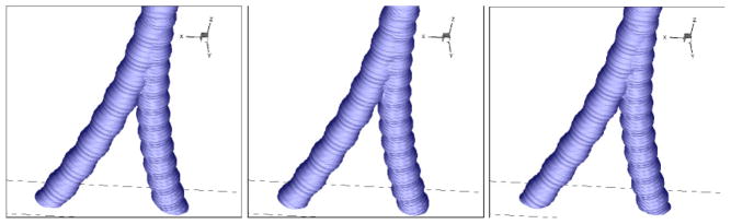
Finally, an example computation is presented in Fig. 13 at a volumetric flow rate of liter/min, as would be exerted during heavy breathing or light cough. The mucin active link lifetime is τ₀=0.5 s as in Fig. 12, hence the results are indicative of effect of high core flow speed upon clearance of mucus.

Fig. 13.

Sequence of interface shapes at high flow rates.

7 Conclusions

A multiscale computational procedure has been introduced for the problem of multiphase core-annular flow in airways, one phase exhibiting gel-like behavior, the other Newtonian fluid behavior. Overall bulk transport in the airway is captured by a one-dimensional representation through airway segments and junctions. Loss mechanisms, viscoelastic behavior, and momentum transfer between phases are computed using a kinetic representation based upon probability density functions for the state of each phase. A novel lattice Fokker-Planck methodology is introduced in which the relaxation behavior of polymers comprising the mucin network is described by minimization of a functional capturing both the deterministic effects of response to flow shear and polymer entropic forces, but also the effect of random background excitation of the mucin polymer network by thermal motions of the solvent. An efficient evaluation of the relaxation operator is achieved by concurrent simulation of stochastic differential equations using massively parallel graphics processing units.

The application of the continuum-kinetic-microscopic interaction procedure has been shown to lead to different entrainment-induced clearance behavior when microscopic parameters describing the formation and destruction of mucin cross-links are changed. The models considered in this work are simple by comparison to the true biochemistry of mucins in the airway surface liquid, but the algorithm introduced here allows linkage of widely disparate spatial scales, and is a promising tool in the classification of importance of microscopic parameters upon overall flow clearance. The main objective of this work has been to introduce the theoretical concepts and algorithmic framework to qualitatively show that microscopic effects can be linked to continuum level clearance behavior, and further work is underway to quantitatively validate the numerical predictions.

Limitations

The multiscale algorithm introduced in this paper is constrained by a number of modeling choices.

1. Kinetic mucus model. The rheology of mucus, especially at higher (e.g. 4–8%) mucin concentrations, is considerably more complex than the model used here that concentrates on simple density estimates of active and dangling links. The topology of the links becomes important when attempting to characterize polymer entagled states. Capturing this complexity would require probability distribution functions for a larger set of variables than the simple link deformation length model used here. Lattice representations would still be possible, but rapidly increase in complexity.

2. Flow reconstruction procedure. A simple, one-dimensional segment and junction model was adopted to capture overall momentum transport, and forms the basis for reconstructing a representative flow configuration for the kinetic-level lattice methods. Such an approach is incapable of representing large scale flows that deviate significantly from an axisymmetric airway surface liquid configuration. An example would be meandering rivulets of mucus that are observed experimentally, and would only partially ocupy the surface area of a segment.

References

- 1.Bai R, Kelkar K, Joseph DD. Direct simulation of interfacial waves in a high-viscosity-ratio and axisymmetric core-annular flow. Journal of Fluid Mechanics. 1996;327:1–34. [Google Scholar]
- 2.Bai RY, Chen KP, Joseph DD. Lubricated pipelining - stability of core annular-flow .5. experiments and comparison with theory. Journal of Fluid Mechanics. 1992;240:97–132. [Google Scholar]
- 3.Bansil R, Stanley E, Lamont JT. Mucin biophysics. Annual Review of Physiology. 1995;57:635–657. doi: 10.1146/annurev.ph.57.030195.003223. [DOI] [PubMed] [Google Scholar]
- 4.Bird RB, Curtiss CF. Molecular theory expressions for the stress tensor in flowing polymeric liquids. Journal of Polymer Science-Polymer Symposia. 1985;(73):187–199. [Google Scholar]
- 5.Blake J. Movement of mucus in lung. Journal of Biomechanics. 1975;8(3–4):179–190. doi: 10.1016/0021-9290(75)90023-8. [DOI] [PubMed] [Google Scholar]
- 6.Bonvin J, Picasso M. Variance reduction methods for connffessit-like simulations. Journal of Non-Newtonian Fluid Mechanics. 1999;84(2–3):191–215. [Google Scholar]
- 7.Brackbill JU, Kothe DB, Zemach C. A continuum method for modeling surface-tension. Journal of Computational Physics. 1992;100(2):335–354. [Google Scholar]
- 8.Bromberg LE, Barr DP. Self-association of mucin. Biomacromolecules. 2000;1(3):325–334. doi: 10.1021/bm005532m. [DOI] [PubMed] [Google Scholar]
- 9.Carlstedt I, Sheehan JK, Corfield AP, Gallagher JT. Mucous glycoproteins - a gel of a problem. Essays in Biochemistry. 1985;20:40–76. [PubMed] [Google Scholar]
- 10.Chen K, Joseph DD. Lubricated pipelining - stability of core annular-flow .4. ginzburg-landau equations. Journal of Fluid Mechanics. 1991;227:587–615. [Google Scholar]
- 11.Cifre JGH, Barenbrug Tmaom, Schieber JD, van den Brule Bhaa. Brownian dynamics simulation of reversible polymer networks under shear using a non-interacting dumbbell model. Journal of Non-Newtonian Fluid Mechanics. 2003;113(2–3):73–96. [Google Scholar]
- 12.Clarke SW, Jones JG, Oliver DR. Resistance to 2-phase gas-liquid flow in airways. Journal of Applied Physiology. 1970;29(4):464. doi: 10.1152/jappl.1970.29.4.464. [DOI] [PubMed] [Google Scholar]
- 13.Espinosa FF, Kamm RD. Thin layer flows due to surface tension gradients over a membrane undergoing nonuniform, periodic strain. Annals of Biomed Engg. 1997;25:913–925. [PubMed] [Google Scholar]
- 14.Groot RD, Agterof WGM. Monte-carlo study of associative polymer networks .1. equation of state. Journal of Chemical Physics. 1994;100(2):1649–1656. [Google Scholar]
- 15.Groot RD, Agterof WGM. Monte-carlo study of associative polymer networks .2. rheologic aspects. Journal of Chemical Physics. 1994;100(2):1657–1664. [Google Scholar]
- 16.Grotberg JB. Pulmonary flow and transport phenomena. Annual Review of Fluid Mechanics. 1994;26:529–571. [Google Scholar]
- 17.Grunau D, Chen SY, Eggert K. A lattice boltzmann model for multiphase fluid-flows. Physics of Fluids a-Fluid Dynamics. 1993;5(10):2557–2562. [Google Scholar]
- 18.Gunstensen AK, Rothman DH, Zaleski S, Zanetti G. Lattice boltzmann model of immiscible fluids. Physical Review A. 1991;43(8):4320–4327. doi: 10.1103/physreva.43.4320. [DOI] [PubMed] [Google Scholar]
- 19.Hofmann W, Koblinger L. Monte-carlo modeling of aerosol deposition in human lungs .2. deposition fractions and their sensitivity to parameter variations. Journal of Aerosol Science. 1990;21(5):675–688. [Google Scholar]
- 20.Houtmeyers E, Gosselink R, Gayan-Ramirez G, Decramer M. Regulation of mucociliary clearance in health and disease. European Respiratory Journal. 1999;13(5):1177–1188. doi: 10.1034/j.1399-3003.1999.13e39.x. [DOI] [PubMed] [Google Scholar]
- 21.Jordan R, Kinderlehrer D, Otto F. The variational formulation of the fokker-planck equation. Siam Journal on Mathematical Analysis. 1998;29(1):1–17. [Google Scholar]
- 22.Jordan R, Kinderlehrer D, Otto FD, Joseph D, Bai R, Chen KP, Renardy YY. Core-annular flows. Annual Review of Fluid Mechanics. 1997;29:65–90. [Google Scholar]
- 23.Jourdain B, Le Bris C, Lelievre T. On a variance reduction technique for micro-macro simulations of polymeric fluids. Journal of Non-Newtonian Fluid Mechanics. 2004;122(1–3):91–106. [Google Scholar]
- 24.Kang M, Shim H, Osher S. Level set based simulations of two-phase oil-water flows in pipes. Journal of Scientific Computing. 2007;31(1–2):153–184. [Google Scholar]
- 25.Kesimer M, Makhov AM, Griffith JD, Verdugo P, Sheehan JK. Unpacking a gel-forming mucin: a view of muc5b organization after granular release. American Journal of Physiology-Lung Cellular and Molecular Physiology. 2010;298(1):L15–L22. doi: 10.1152/ajplung.00194.2009. [DOI] [PMC free article] [PubMed] [Google Scholar]
- 26.Kim CS, Iglesias AJ, Sackner MA. Mucus clearance by 2-phase gas-liquid flow mechanism - asymmetric periodic-flow model. Journal of Applied Physiology. 1987;62(3):959–971. doi: 10.1152/jappl.1987.62.3.959. [DOI] [PubMed] [Google Scholar]
- 27.Kim CS, Rodriguez CR, Eldridge MA, Sackner MA. Criteria for mucus transport in the airways by 2-phase gas-liquid flow mechanism. Journal of Applied Physiology. 1986;60(3):901–907. doi: 10.1152/jappl.1986.60.3.901. [DOI] [PubMed] [Google Scholar]
- 28.King M, Chang HK, Weber ME. Resistance of mucus-lined tubes to steady and oscillatory air-flow. Journal of Applied Physiology. 1982;52(5):1172–1176. doi: 10.1152/jappl.1982.52.5.1172. [DOI] [PubMed] [Google Scholar]
- 29.Knowles MR, Boucher RC. Mucus clearance as a primary innate defense mechanism for mammalian airways. Journal of Clinical Investigation. 2002;109(5):571–577. doi: 10.1172/JCI15217. [DOI] [PMC free article] [PubMed] [Google Scholar]
- 30.Kupferman R, Shamai Y. Spatially correlated noise and variance minimization in stochastic simulations. Journal of Non-Newtonian Fluid Mechanics. 2009;157(1–2):92–100. [Google Scholar]
- 31.Lai SK, Wang YY, Wirtz D, Hanes J. Micro- and macrorheology of mucus. Advanced Drug Delivery Reviews. 2009;61(2):86–100. doi: 10.1016/j.addr.2008.09.012. [DOI] [PMC free article] [PubMed] [Google Scholar]
- 32.LeVeque RJ. Finite Volume Methods for Hyperbolic Problems. Cambridge University Press; 2002. [Google Scholar]
- 33.Li J, Renardy Y. Direct simulation of unsteady axisymmetric core-annular flow with high viscosity ratio. Journal of Fluid Mechanics. 1999;391:123–149. [Google Scholar]
- 34.Lishchuk SV, Care CM, Halliday I. Lattice boltzmann algorithm for surface tension with greatly reduced microcurrents. Physical Review E. 2003;67(3) doi: 10.1103/PhysRevE.67.036701. [DOI] [PubMed] [Google Scholar]
- 35.Malaspinas O, Fietier N, Deville M. Lattice boltzmann method for the simulation of viscoelastic fluid flows. Journal of Non-Newtonian Fluid Mechanics. 2010;165(23–24):1637–1653. [Google Scholar]
- 36.McCullagh CM, Jamieson AM, Blackwell J, Gupta R. Viscoelastic properties of human tracheobronchial mucin in aqueous-solution. Biopolymers. 1995;35(2):149–159. doi: 10.1002/bip.360350203. [DOI] [PubMed] [Google Scholar]
- 37.Nordgard CT, Draget KI. Oligosaccharides as modulators of rheology in complex mucous systems. Biomacromolecules. 2011;12(8):3084–3090. doi: 10.1021/bm200727c. [DOI] [PubMed] [Google Scholar]
- 38.Nourgaliev RR, Dinh TN, Theofanous TG, Joseph D. The lattice boltzmann equation method: theoretical interpretation, numerics and implications. International Journal of Multiphase Flow. 2003;29(1):117–169. [Google Scholar]
- 39.Onishi J, Chen Y, Ohashi H. Dynamic simulation of multi-component viscoelastic fluids using the lattice boltzmann method. Physica a-Statistical Mechanics and Its Applications. 2006;362(1):84–92. [Google Scholar]
- 40.Ottinger HC, vandenBrule Bhaa, Hulsen MA. Brownian configuration fields and variance reduced connffessit. Journal of Non-Newtonian Fluid Mechanics. 1997;70(3):255–261. [Google Scholar]
- 41.Owens RG, Phillips TN. Computational Rheology. Imperial College Press; 2005. [Google Scholar]
- 42.Scherer PW, Burtz L. Fluid mechanical experiments relevant to coughing. Journal of Biomechanics. 1978;11(4):183–187. doi: 10.1016/0021-9290(78)90011-8. [DOI] [PubMed] [Google Scholar]
- 43.Siamas GA, Jiang X, Wrobel LC. Dynamics of annular gas-liquid two-phase swirling jets. International Journal of Multiphase Flow. 2009;35(5):450–467. [Google Scholar]
- 44.Succi S. The Lattice Boltzmann Equation for Fluid Dynamics and Beyond. Clarendon Press; 2001. [Google Scholar]
- 45.Tanaka F, Edwards SF. Viscoelastic properties of physically cross-linked networks - transient network theory. Macromolecules. 1992;25(5):1516–1523. [Google Scholar]
- 46.Vaccaro A, Marrucci G. A model for the nonlinear rheology of associating polymers. Journal of Non-Newtonian Fluid Mechanics. 2000;92(2–3):261–273. [Google Scholar]
- 47.Winnik MA, Yekta A. Associative polymers in aqueous solution. Current Opinion in Colloid and Interface Science. 1997;2(4):424–436. [Google Scholar]