Peptide crystal simulations reveal hidden dynamics

Abstract

Molecular dynamics simulations of biomolecular crystals at atomic resolution have the potential to recover information on dynamics and heterogeneity hidden in the X-ray diffraction data. We present here 9.6 microseconds of dynamics in a small helical peptide crystal with 36 independent copies of the unit cell. The average simulation structure agrees with experiment to within 0.28 Å backbone and 0.42 Å all-atom rmsd; a model refined against the average simulation density agrees with the experimental structure to within 0.20 Å backbone and 0.33 Å all-atom rmsd. The R-factor between the experimental structure factors and those derived from this unrestrained simulation is 23% to 1.0 Å resolution. The B-factors for most heavy atoms agree well with experiment (Pearson correlation of 0.90), but B-factors obtained by refinement against the average simulation density underestimate the coordinate fluctuations in the underlying simulation where the simulation samples alternate conformations. A dynamic flow of water molecules through channels within the crystal lattice is observed, yet the average water density is in remarkable agreement with experiment. A minor population of unit cells is characterized by reduced water content, 3₁₀ helical propensity and a gauche(−) side-chain rotamer for one of the valine residues. Careful examination of the experimental data suggests that transitions of the helices are a simulation artifact, although there is indeed evidence for alternate valine conformers and variable water content. This study highlights the potential for crystal simulations to detect dynamics and heterogeneity in experimental diffraction data, as well as to validate computational chemistry methods.

1 Introduction

X-ray crystallography has played the essential role in the development of the field of structural biology. In doing so, the conventional focus of biomolecular x-ray crystallography has been on identifying a single structure to represent the molecule that best explains the collected diffraction data. Yet, it is well established that biomolecules, both in solution and in crystal, are highly dynamic objects which populate an ensemble of structurally heterogeneous states.¹ Information on this dynamicity and heterogeneity is “hidden” in the experimental data set which, by its nature, is essentially time and space averaged.² In recent years, several attempts have been made to develop methods to mine the experimental data for information on dynamics and structural heterogeneity in the protein.^3,4 Here we present a further advance in this direction by employing the power of all atom, explicit solvent, molecular dynamics (MD) simulations of crystals to gain a more exact and time-resolved picture of a the inner dynamics of a peptide crystal. Crystallographic refinements against the computed average electron density are critically compared against refinements against the experimental density.

The potential of computer simulations to extend our understanding of the motions of biomolecules beyond the experimental images offered by X-ray crystallography or NMR experiments has driven the application of computational techniques to problems in structural biology. It is now feasible to simulate protein systems containing hundreds of residues for microseconds of real time. Commensurate with improved simulation algorithms and computer hardware, the molecular models have been scrutinized for their dynamic, equilibrium thermodynamic and structural characteristics. In many respects, the models perform realistically^5,6,7,8, but by pressing the models to jump from reproducing known results to correctly predicting new data^9,10, the models also show signs of over-fitting and reduced transferability. Peptide and protein crystals offer a rich set of experimental data and the opportunity to subject molecular models to tests in which the time-averaged positions and fluctuations of atoms are known.

The applicability of simulations to the interpretation and even improvement of X-ray data sets is a goal on the horizon. More immediately, efforts have been focused on tailoring simulations to match crystallization conditions and devising appropriate analyses to directly compare molecular models with crystallized biomolecules.^11,12,13 Crystallographic data have also been used to validate computational results in many forms.¹⁴ One of the challenges of simulating crystals lies in the necessity to extrapolate the unknown crystal solvent content. It remains a high priority to select systems with as little uncertainty in the crystallization solution as possible. Our previous simulations^15,16,17 were among the longest crystal simulations performed at the time, but even with 8 to 12 independent copies of the unit cell, and hundreds of nanoseconds of simulation, some of the most interesting parameters, such as the persistence of hydrogen bonds and density of material near crystallographic water sites, were not sufficiently converged to determine whether the simulation matched the X-ray data.

In this study we present simulations of the crystallized deca-peptide hereafter referred to as “fav8”.¹⁸ The sequence of this synthetic peptide favors helix formation and aromatic intermolecular interactions. Furthermore, the crystal is exceptionally dry, with only four waters placed in the experimental electron density with only four waters placed in the original refinement and no room for disordered “bulk” solvent. As we show in the results, the unit cell volume is correctly maintained by including only the four crystal water molecules. The ability to simulate the entire fav8 deca-peptide crystal lattice with certainty about its material composition for microseconds enables us to compare the simulation and the X-ray diffraction data in unprecedented detail. We perform several simulations, the longest of which reached 2.4 microseconds, of an extended fav8 lattice comprising 36 independent unit cells—in all, roughly ten times the simulation length of our previous simulations with ten times the number of independent unit cells. The results give a much clearer picture of the time-averaged solvent density, solvent diffusion within the peptide lattice, and hydrogen bonding for maintaining peptide structure.

2 Methods

2.1 Preparation of the simulation supercell

Atomic coordinates were taken from the cif format file in the supplemental data of the publication that reported the molecule's structure.¹⁸ This is a synthetic decapeptide (sequence Boc-Aib-Ala-Phe-Aib-Phe-Ala-Val-Aib-Ome) designed to fold in a helical conformation with aromatic t-stacking interactions between phenylalanine rings of separate monomers in its crystallized form. In the decapeptide, Aib (α-aminoisobutyryl) is a non-standard amino acid (alanine modified by methylation of the Cα hydrogen) and Boc (N-tert-butoxycarbonyl) and Ome (O-methyl ester) are terminal blocking groups. The peptide formed crystals in the P1 space group, with one asymmetric unit (ASU) per triclinic unit cell of dimensions a=10.802, b=16.361, c=17.853 Å, α=116.405°, β=95.535°, and γ=93.164°. The ASU consists of two nonequivalent decapeptides, referred to as monomer A (residues A1 to A10) and monomer B (residues B1 to B10), as well as four crystallographic water oxygen positions. The diffraction experiment was carried out at a temperature of 294 K. The major structural features of the unit cell include phenylalanine side chain π and t-stacking interactions as discussed in the original publication; four crystallographic water molecules lie within hydrogen bonding distance of each other and of the N- and C-termini of adjacent decapeptides.

A “supercell” of 4 × 3 × 3 unit cells was created by using the PropPDB module of the Amber11 package¹⁹, measuring 43.208 × 49.083 × 53.559 Å and comprising 72 copies of the fav8 decapeptide. Views of the supercell along the three crystal vectors are shown in Fig. 1. Inspection of the supercell shows that crystal packing places the crystallographic waters clusters in interstices, connected to one another with little steric hindrance between adjacent unit cells forming channels along the a vector of the crystal lattice.

Figure 1.

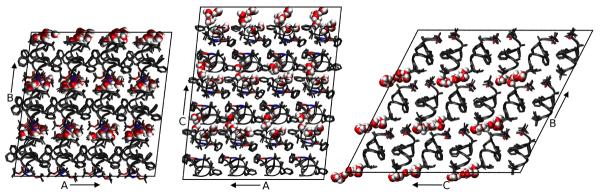
Three views of the simulated fav8 crystal lattice. 36 unit cells are stacked in a 4 × 3 × 3 arrangement in the triclinic super-system; each unit cell comprises two fav8 decapeptide helices arranged roughly parallel to one another. Each view looks down one axis of the lattice; borders of the simulated system are marked in black lines. The peptide backbone is shown in ribbons, or in licorice form in the case of Aib and terminal blocking residues. Water molecules are illustrated in space-filling form; we find that the water forms continuous channels running through the lattice along the a axis.

In previous all-atom crystal simulations^15,16,17, solvent that was unaccounted for in the X-ray data was added to the simulation supercell until the experimental volume of the crystal was accurately reproduced by molecular dynamics at the temperature and pressure of the crystal growth conditions. Furthermore, different species of solvent were added in proportions to mimic the composition of the crystal mother liquor. In the case of fav8, initial equilibration and trial molecular dynamics production runs reproduced crystal lattice parameters accurately without any additional solvent. Therefore, we performed all production runs with only the molecules found in the original cif file.

2.2 Molecular dynamics simulations

Protonation of the peptide structure and construction of molecular topology and coordinate files for the crystal supercell was done using the tleap module of Amber11 and Reduce.²⁰ The peptide in the simulation supercell was modeled using parameters of the Amber ff99SB force field²¹ and the TIP3P water model.²² The Boc, Aib, and Ome residues are not found in the standard Amber force field, but we obtained charges for these residues using RESP fitting²³ and took other parameters from similar compounds described by ff99SB; details are in the Supplementary Material.

System optimization, equilibration, and production dynamics were performed using the PMEMD module of AMBER11. When the system volume was allowed to vary, constant pressure was maintained by a Berendsen barostat²⁴ with isotropic pressure scaling (At the time this study was conducted, anisotropic scaling was not available in Amber for a triclinic box. This feature has since been added). Constant temperature was maintained during all dynamics with a Langevin thermostat²⁵ (collision frequency of 1/ps) at the experimental crystal diffraction temperature of 294 K. To avoid artifacts arising from the reuse of the same random number sequences,²⁶ a different random number generator seed was used each time a simulation was restarted. Force calculations were performed with a 9.0 Å real space cutoff in the context of periodic boundary conditions, smooth particle-mesh Ewald electrostatics,^27,28 and a homogeneity assumption for long-range van der Waals contributions. The SHAKE²⁹ and SETTLE³⁰ algorithms were used to constrain the lengths of bonds to hydrogen and the internal geometry of rigid water molecules, respectively.

System equilibration was carried out using the following scheme. First, the conformations of peptide residues, including added hydrogens, were relaxed via 100 steps of steepest descent optimization followed by 900 steps of conjugate gradient optimization with 256 kcal/(mol-Ų) position restraints applied to solvent molecules. Next, the entire system was optimized in the same manner but with no restraints. Initial restrained dynamics were performed at constant volume for 50 ps with a 1.0 fs time step and 256 kcal/(mol-Ų) restraints on all peptide heavy atoms, followed by another 225 ps of restrained dynamics at a 1.5 fs time step during which restraints were gradually reduced to 4.0 kcal/(mol-Ų). Next, restrained dynamics were performed at a pressure of 1 bar for 400 ps using a 2 fs time step as restraints on peptide heavy atoms were gradually relaxed from 4.0 to 0.0625 kcal/(mol-Ų). Unrestrained production dynamics were propagated at a 2 fs time step, matching the final phase of equilibration in which all restraints had been reduced to zero.

Production simulations were carried out on clusters of 48-core 2.2GHz Opteron CPUs provided by the Rutgers BioMaPS High-Performance Computing facility and also on a private cluster of serial GPUs. A total of 4 simulations were propagated for 1.6 to 2.4 microseconds each.

2.3 Analysis of data

Data analysis was carried out using in-house scripts and the Amber11 ptraj module for MD trajectory analysis. Two root mean square deviation (RMSD) metrics which we refer to as “ASU RMSD” and “lattice RMSD” were calculated using the Kabsch algorithm.^31,32 They are described briefly in section 3.1 and more details can be found in Ref.15. Secondary structure was determined using the DSSP³³ algorithm. Experimental electron density maps were calculated from experimental intensities kindly provided by S. Aravinda and P. Balaram, coordinates and anisotropic displacement parameters found in the Supplementary Data of Aravinda et al., 2003 by zero-cycle unrestrained maximum likelihood refinement using Refmac.³⁴ Molecular refinement was performed with Phenix.^35,36The Visual Molecular Dynamics (VMD) program³⁷ and ccp4mg³⁸ were used for visualization and image generation. Approaches to calculating B-factors are described in the Results section.

To calculate average simulation electron density and structure factors, an evenly-spaced selection of 4000 snapshots was taken from the final 2 μs of the longest of our simulation trajectories, amounting to 144,000 conformations of the ASU. Electron density maps were generated directly from each of these conformations using the CCP4 program SFALL.^39,40 For each map-generation run, all 36 unit cells for the given time point were included in the calculation using a unit cell repeat that was an integral reduction of the simulation cell. For any given time point in the simulation the B-factors of all the atoms are formally zero, but this presents certain problems in calculating electron density because the constant “c” term in the conventional Cromer-Mann reciprocal-space atomic form factor tables⁴¹ becomes a Dirac delta-function in real space. This results in a singularity when plotting the electron density onto a grid for the fast Fourier transform calculation of the structure factors.⁴⁰ To avoid this singularity a B-factor of 15 was assigned to all atoms (large enough to avoid aliasing errors) before calculating the electron density maps. Despite the slightly different cells (due to simulation in the NPT ensemble, see Results 3.1), all of these maps were calculated to have the same number of grid points: 96×108×120.

Structure factors were calculated from each of these maps, and the translation needed to optimally superimpose each time point in the simulation onto the published structure was determined by deconvolution in reciprocal space. This was necessary because the “origin” is not restrained and drifts slowly throughout the simulation, so that averaging electron density in real space (or structure factors with phases in reciprocal space) would eventually “blur” itself down to a constant (the average electron density of the crystal), driving all structure factors to zero. Specifically, the complex structure factors calculated from the published atomic coordinates were divided by the complex structure factors obtained from the electron density of the simulation time point. The map calculated from these “quotient” structure factors is the correlation function of the two parent maps, and the tallest peak in this map is located at the optimal translation to “align” them.

After determining these optimal shifts, the atoms from each simulation time point were translated appropriately, and the electron density maps re-calculated. The average of all these electron-density maps was then taken and a final Fourier transform was computed to obtain the expected structure factors of a single crystal mosaic domain comprised of all 144000 ASUs represented in the trajectory. The CCP4 program CAD was used to remove the contribution of the B-factor=15 from the structure factors. The R-factor of these simulation structure factors with the observed structure factors was calculated after applying an optimal scale and B-factor with the CCP4 program SCALEIT.39,42

3 Results and Discussion

Dynamics of the fav8 peptide crystal lattice were analyzed on the microsecond timescale in a system comprising 36 unit cells stacked 4×3×3. Simulations were run in quadruplicate (one 2.4 μs trajectory, and three additional 1.6 μs trajectories). The simulated system retained the unit cell angles and aspect ratios of the crystal due to the isotropic pressure rescaling of cell dimensions, but the corresponding atoms in each of the 36 unit cells were otherwise allowed to move independently. In addition to structural comparisons, we computed isotropic B-factors for all peptide heavy atoms and again found close agreement with the experiment. Finally, we turned our attention to dynamics of water molecules and found them to migrate between different unit cells, indicating that the electron density of water molecules in the fav8 crystal arises from many distinct molecules interchanging positions during the experiment.

3.1 Comparison to experimental structure

It is less straightforward than one might think to quantify the agreement between a crystal lattice simulation and the refined structure inferred from X-ray diffraction data. Unit cell volume, positional RMSD, average unit cell structure and thermal vibrations provide a strong set of indicators as to the simulation's accuracy. Positional RMSD was measured in two distinct ways. First, we define “ASU RMSD” as:

$$\text{ASURMSD}=\sqrt{\frac{1}{M}\sum _{i=1,M}\left[\frac{1}{N}\sum _{j=1,N}{\mid r_{i,j}-r_{i,j}\mid }^2\right]}$$

where the inner summation runs over N atoms, the outer summation runs over M ASUs, r_{i, j} is the position vector of an atom in the simulation snapshot, $r_{i,j}^y$ is the experimentally determined position vector of that atom, and the statistic is calculated after rotational and translational alignment of the backbone heavy atom coordinates in each ASU against the crystal fav8 structure using the Kabsch algorithm.³¹ This RMSD, which was computed for backbone and side-chain atoms (with provisions for the symmetry of atoms in Phe rings and the Boc terminus), accounts for all disorder arising from bending and distortion of individual fav8 monomers and disorder arising from changes in the contacts between the pair of monomers that composes each ASU. Second, we compute a “Lattice RMSD” which follows the same formula as the ASU RMSD; however in this case ASUs are not aligned in the traditional manner. Instead, ASU's are superimposed by first center of mass aligning each supercell and then reversing the translational space group operations by which the simulation supercell was constructed. The center of mass alignment is necessary due to translational drift of the origin of the supercell, since its potential energy is translationally invariant. This metric captures rigid-body librations of the peptides in the unit cell and lattice distortion between fav8 monomers in different unit cells, since atoms in different unit cells are not constrained to move in any symmetric fashion. Figure 2 plots these RMSD measurements over the course of the 2.4 μs trajectory. If one focuses on a much shorter timescale, the RMSD of both the backbone and of the side-chain atoms appears to converge to 0.5/0.7 Å after as little as 20ns of dynamics, but Figure 2 shows that these metrics rise suddenly at 400 ns to 0.6/0.75 Å, levels which are maintained for the remainder of the simulation. (Convergence of the other three trajectories is illustrated in Suppl. Data Fig. S1; backbone and side-chain RMSD in these simulations is comparable to that of the 2.4 μs trajectory.) Also after roughly 400 ns, backbone lattice RMSD converges to about 0.75 Å. RMSD adds in quadrature and therefore these results indicate that there is an approximately equal contribution to overall RMSD from intra- and inter-molecular distortions. All further analyses were performed after discarding the first 400 ns of simulation.

Figure 2.

Positional RMSDs of heavy atoms relative to the X-ray structure. Details of each metric are given in the main text; all quantities are plotted over the course of a 2.4 μs simulation, and plots for three additional 1.6 μs simulations are given in the supporting information. Purple: ASU RMSD for backbone (N,CA,C) atoms. Orange: ASU RMSD for side-chain heavy atoms. Blue: lattice RMSD for backbone atoms.

The crystallographic raw data is a diffraction pattern that is the averaged result over time and over three dimensional space of the repeating unit cell. To set our analysis in line with the experimental results, we calculated an average structure of the simulated unit cells using the same reverse symmetry operations and Phe/Boc atom equivalencies that had been used to compute lattice and ASU RMSDs. A superposition of the resulting average structure with the X-ray result is shown in Figure 3. The RMSD of backbone and side chain heavy atoms for this average structure is 0.32/0.45 Å, which is much lower than the RMSD of the individual snapshots cited above. Thus, structural deviations can occur at instantaneous snapshots of the simulation while the time-averaged structure maintains close similarity to the x-ray model, as is consistent with a dynamic interpretation of the crystal. In the average structure, monomer A agrees nearly perfectly (0.15/0.17 Å backbone/side chain RMSD) with the refined X-ray structure, and only the C-terminus of monomer B (residues B8-B10) is seen to deviate significantly (residues A1-B7 0.20/0.21 Å, residues A1-B8 0.21/0.38 Å, residues A1-B9 0.29/0.44 Å; indicating disorder in only the side chain of residue B8 and in both backbone and side chain of residues B9/B10). As shown in the Supporting Information Figure S3, the deviations in monomer B are in fact confined to a subset of 9 of the 36 unit cells. The average heavy atom RMSD of monomer B in this subset is 0.84 Å while in the remaining cells it is 0.51 Å; (for comparison, the average RMSD of monomer A in all cells is 0.23 Å). Furthermore, if the C-terminus (residues B8-B10) is removed from the calculation, the RMSD of the subset of 9 unit cells drops from 0.84 to 0.63 Å and for the remaining cells from 0.51 to 0.23 Å, identical to the average RMSD of monomer A (0.23 Å). As is evident in Fig. 3, and is discussed more fully below, the simulation reflects an ensemble of two structural populations characterized by differences at the C-terminus of monomer B.

Figure 3.

Superposition of the average simulated structure (black) against the structure refined from diffraction data (orange). The first decapeptide (monomer A) matches the X-ray data closely; monomer B deviates in the side-chain conformation of its Val residue and in the helicity of its C-terminal backbone residues 16–20.

Direct comparison of electron densities provides a more useful criterion for a structural comparison of the simulation against experiment, since it is X-ray scattering from an average density that determines the intensities of the observed diffraction peaks. For this, we calculated the electron density of 4000 evenly-spaced snapshots taken from the simulation trajectory, amounting to 144,000 conformations of the ASU. The electron densities were optimally aligned to the crystallographic origin as described in the methods section to account for the slow drift of the origin during the simulation. The average of all these electron-density maps was then taken and a final Fourier transform computed to obtain the expected structure factors of a single crystal mosaic domain comprised of 144000 ASUs. Comparison to the observed structure factors using the CCP4 program SCALEIT,39,42 resulted in best-fit scale=1.09 and B=−0.7948, indicating that the overall Wilson B factor of the real crystal was remarkably similar to that predicted by the simulation. The R factor of these calculated structure factors with the observed structure factors was 28% to 1.0 Å resolution and 21% to 2.0 Å resolution. After applying the 4-sigma intensity cutoff traditionally employed when computing R factors for small molecules, the agreement of our simulation-averaged structure factors with observed structure factors was 23% to 1.0 Å and 20% to 2.0 Å. This is remarkably good agreement considering that the observed structure factors were not used to bias the simulation run, qualifying this R factor as not just an Rfree43 but as the Rvault statistic proposed by Kleywegt.44 Given the clearly anomalous behavior of the C terminus of the B chain in the simulation some disagreement with the observed structure factors is expected, so the close agreement of the observed structure factors with those predicted by averaging over this un-biased MD simulation is remarkable.

We next refined the fav8 coordinates against the structure factors from the simulation density, which yielded an R-work/R-free of 9.6%/12.1%. This is higher than the reported experimental R-factor of 8%¹⁸ primarily because the simulated crystal has more disorder than the experimental one, as discussed below. This refinement represents an “expected refined structure given the simulation density” and is arguably the best vehicle for making structural comparisons between theory and experiment, since X-ray scattering is determined by the average electron density, and not by any average of the coordinates themselves. Table 1 presents RMSD statistics between this model and coordinates obtained by refinement against experimental density and by the more common procedure of simply averaging the coordinates over the simulation snapshots. (For consistency we use results from our re-refinement against experimental data; the RMSD of our re-refined structure vs. the one originally deposited is 0.04/0.05 Å backbone/side chain.) The RMSD of the simulation-refined model to the experiment-refined model was 0.21/0.30 Å backbone/side chain, which is lower than the values (0.28/0.44 Å) obtained by coordinate averaging. Furthermore, calculation of the mean obtained by comparing simulation snapshots against each of these three structures yield higher RMSDs showing that while instantaneous simulation coordinates can differ to a greater degree from the refined model, the overall simulation average remains close. Therefore, a simulation-refined model provides a good representation of the average simulation structure while avoiding the geometric irregularities incurred with the more commonly employed coordinate averaging.

Table 1.

Root mean square deviation (RMDS) values between various structures. The statistics in each box are the backbone RMSD (first) and the all heavy atom RMSD. Terminal capping residues were excluded from the calculation. “Experiment-refined” is the model obtained from refinement of fav8 against the experimental density in Phenix. “Simulation-refined” is the structure obtained by refinement against the simulation average density. “Simulation average” is the structure composed of the mean coordinates of each atom over the entire length of the 2.4 μs simulation. The last column presents the average backbone/side chain RMSD of all simulation snapshots against the single structure for that row.

	Exp.-refined	Sim.-refined	Sim. average	Average snapshot
Experiment-refined	0.0/0.0	0.205/0.301	0.283/0.423	0.462/1.180
Simulation-refined		0.0/0.0	0.129/0.282	0.387/1.121
Simulation-average			0.0/0.0	0.372/0.822

One global parameter which indicates how well a crystal lattice simulation is reproducing the crystal is its volume. In previous work, we have sought to reproduce this parameter arbitrarily to within 0.3% of the experimental result¹⁵ and found that the choice of simulation models has a significant impact on the outcome.¹⁷ As before, our simulations were performed in an NPT ensemble using a Berendsen barostat and Langevin thermostat. The experimental volume of 2795.8 ų was maintained at a mean of 99.89 ± 0.003% of experiment (Figure 4, Suppl. Data Fig. S2). It is noteworthy that this was achieved without the addition of extra water molecules or other solvent. The fav8 X-ray structure is of high resolution and the unit cell itself is very compact, but perhaps most importantly the unit cell is very dry for a proteinaceous crystal.

Figure 4.

Volume of the supercell over the course of a 2.4 μs simulation. Following an initial settling, the system volume reaches an equilibrium value roughly 0.2% below the volume of the unit cell observed by X-ray diffraction. Instantaneous fluctuations of the volume have amplitudes of an additional 0.2%.

Crystallographic B-factors may be loosely interpreted as indicators of the thermal motion occurring in a crystal structure, but it is more accurate to say that B-factors can arise both from movements of the individual atoms within an ASU (intra-ASU or “local” disorder) as well as from rigid body librations and lattice distortion (inter-ASU or “global” disorder). Isotropic B-factors are related to the mean squared fluctuations of atoms around their average position by the formula⁴⁵

$$B=\frac{\langle u^2\rangle \times 8{\pi }^2}{3}$$

where 〈u²〉 is the three dimensional mean square deviation and B is the thermal isotropic B-factor. In crystallographic refinement models, an atom that is posited to be responsible for the surrounding electron density must exhibit a distribution of positions; this distribution is estimated from the available electron density, and the mean squared fluctuations of the distribution then imply a B-factor. The difference between contributions to the B-factors arising from “local” and “global” disorder, which can be discriminated by molecular dynamics, is related to the difference between calculations of ASU and lattice RMSD.¹⁵ We computed B-factors for the 2.4 μs simulation using both methods as described in Ref. 26. Briefly, “RMSD B-factors” are calculated by first translationally and rotationally fitting each snapshot of each ASU during the trajectory to the crystal ASU and then calculating mean positions and positional variance. “Reverse Symmetry” B-factors are calculated by reversing the translational space group operations by which the simulation supercell was constructed to align each snapshot of each ASU but without any translational/rotational fitting to minimize structural RMSD. The former method thus calculates positional variance stemming from intra-ASU fluctuations while the latter also takes account of contributions from rigid body librations and lattice distortion (i.e departure from crystal symmetry in the relative positions of the ASUs to each other). The computed B-factors are compared to the X-ray model in the left hand side of Figure 5. If global disorder is removed from the calculation (“RMSD B-factors”), the simulation would underestimate the B-factors of most atoms. However, when disorder from rigid body libration is included in the B-factor estimates (“Reverse Symmetry B-factors”), the results for monomer A are in much better agreement with experiment (backbone B-factor RMSD 0.66 vs. 1.73 for RMSD and Reverse Symmetry B-factors respectively). Similar results are observed for monomer B except for C-terminal residues 16–20. These residues undergo changes in their helical state that are coupled to water motion in the crystal lattice (discussed in detail in the following section). The right hand side of Fig. 5 presents the B-factors obtained from refinement against the average simulation density. These are generally in close agreement with the “Reverse Symmetry” B-factors that directly reflect the mean square fluctuations of the coordinates among the simulation snapshots. The refinement-derived and coordinate fluctuation-derived B-factors agree less well in the C-terminus of monomer B, where the simulation samples two different structural conformations. Whereas the coordinate-based B-factor statistic includes the large fluctuations between the two conformations, the refinement algorithm only models one conformation, but its B-factors underestimate the actual magnitude of fluctuations in the underlying simulation. The underlying disorder that is then not reflected in the B-factors gives rise to a higher Rwork/Rfree statistic. Five cycles of occupancy refinement with an alternate conformation for residues 15–20, reflecting the minor population found in the simulation, reduced Rwork/Rfree to 7.7%/9.2% (9.6%/12.1% without the alternate conformation) and converged to a relative occupancy of 71%/29% for the major and minor population of the ensemble, in close agreement with the relative ensemble populations of 72%/28% derived directly from the simulation.

Figure 5.

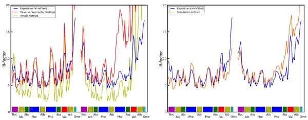
Left-hand plot: Comparison of computed atomic B-factors obtained over the course of the 2.4 μs trajectory to experimental data. “RMSD” B-factors only account for intra-ASU fluctuations and consistently underestimate experimental values. “Reverse symmetry” B-factors account for both local and global (inter-ASU) fluctuations and more closely match experiment. See text for further explanation of the two methods. Right-hand plot: Comparison of B-factors obtained from refinement against the experimental density and against the simulation average density. Backbone atoms are indicated with dots.

3.2 Crystal solvent dynamics

While the RMSD of the peptide converges very quickly in the simulation, the RMSD of the solvent does not converge even after more than two microseconds of simulation. A visualization of the crystal reveals that the packing of the crystal is such that “channels” for water molecules are formed within the crystal. These channels are colinear with lattice vector a and provide little steric hindrance for waters to move between adjacent unit cells. The waters are seen to rapidly diffuse between unit cells through the channels. A careful inspection of the trajectory reveals that the water molecules do not flow smoothly through the channels but rather make sudden hops between positions in adjacent unit cells. Trajectory frames were recorded every 10 ps and in this time water molecules are sometimes seen to move by several Ångstrom.

A diffusion constant was calculated for the water from a linear fit of the cumulative mean square displacement of the waters from their initial position using the Einstein diffusion equation for one dimension:

$$D=\frac{\sum _i{\left[r_i\right(t+\Delta t)-r_i(t\left)\right]}^2}{2\Delta t}$$

Plots of the mean square displacement in each direction of space, shown in Figure 6 and Suppl. Data Fig. S8, do indeed demonstrate that the water is dynamic along the channels while it is restrained from moving in other directions by the channel walls. The channels can be estimated to be 3–4 Å wide based on a converged mean square displacement of about 12 Ų in the directions perpendicular to the channel axis. Diffusion along the channel in the four simulations ranged from 1×10⁻⁸ to 3.4×10⁻⁸ cm²/s, with a mean diffusion rate of 2.5×10⁻⁸ cm²/s calculated after discarding the first 400ns of each trajectory for equilibration. This is roughly 2000 times slower than the reported 5.2×10⁻⁵ cm²/s diffusion constant of TIP3P water⁴⁶ and 1000 times slower than the experimental diffusion constant of liquid water at the same temperature: the waters are dynamic in the simulation, but movement through the channels is constricted. Some variability in water diffusion is evident, as a function of time, in each of the four simulations and particularly in the 2.4 μs trajectory: over the first 400–500ns, a diffusion constant of 3.6×10⁻⁸ cm²/s could be calculated, but the rate abruptly changed to 1.0×10⁻⁸ cm²/s thereafter. A possible connection between these abrupt changes and the disorder in the C-terminus of monomer B is explored later in the Results.

Figure 6.

Mean square displacements (msd) of water molecules over the course of three 1.6 μs and one 2.4 μs simulation trajectories. The slope of the linear fit used to compute the diffusion coefficient is shown in box.

Further analysis in Figure 7 shows that the water molecules occupy several distinct sites within each unit cell along a channel. Hydrogen bonding between water molecules or to peptide backbone atoms is expected to be the primary determinant of these energy minima. Although the average number of waters per unit cell is set to be four in our simulation, the water dynamics produce a heterogeneous population of individual unit cell states: at any given time unit cells may contain as few as zero and as many as eight water molecules. A histogram of the water states occurring throughout the simulation (Figure 7) shows that although 4 is the average state, 5 is in fact the most populous water state. A direct comparison of the cumulative water density from simulation (Figure 8, Panel A) to the experimental electron density (Figure 8, Panel B) reveals close correspondence between the simulation and X-ray data. In both the simulated and experimental structures, two crystallographic waters are located centrally within a compact and spherical lobe of the simulated density while the other two crystallographic waters are located on smeared, dumbbell-shaped regions of density. Correspondingly, these waters also have 3 times higher experimental B-factors. Both images also reveal a fifth area of water density. No specific water was attributed to this density in the X-ray structure, but a partial water occupancy at this position is indicated by the frequently occurring 5-water state (Figure 7) and is consistent with the experimental electron density. Furthermore, a meticulous strategy of free refinement of water occupancy identified 17 putative water peaks and converged to a total of 61 electrons or 6 water molecules altogether. The final Rwork/Rfree statistics for this model were 4.1%/5.8% compared to 6.5%/9.2% for refinement of the 4-water model. Therefore, although exchange of the water molecules between unit cells is not directly reflected in the refined fav8 structure, a model in which exchanges and migration occur continuously is fully consistent with the X-ray diffraction data and leads to improved agreement with the observed structure factors.

Figure 7.

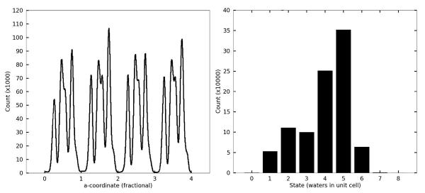
Water densities in the channels observed in simulations. The left-hand panel depicts the density of waters as a function of the a crystal vector coordinate, summed over all nine channels running across the simulation box. The abscissa is numbered according to unit cell fractional coordinates. The right-hand panel plots a histogram of times which each unit cell in the simulation was observed to be associated with a particular number of waters during the 2.4 μs trajectory.

Figure 8.

Water density observed in the 2.4 μs simulation, obtained by using crystal symmetry operations to superimpose all simulated waters onto a single unit cell. Crystallographic peptide is shown in orange/yellow and crystallographic water oxygens as red spheres. Left-hand panel shows the simulated water density (mesh encloses 90% of water density), right-hand panel shows the electron density obtained by X-ray diffraction (2mFo-DFcalc map at 0.8 sigma). Green arrows point to crystallographic waters and indicate their experimental B-factors, purple arrow shows a fifth lobe of water density (see text). Produced with VMD and ccp4mg.

To investigate the tendency of unit cells to take on varying amounts of water, residence times were calculated for each of the water states. We used different smoothing windows to eliminate noise, but regardless of the smoothing window, the one water state exhibits by far the longest residence time (Figure 9). Closer examination of individual water cells revealed that unit cells were rarely occupied by only a single water, but when such dry states did occur they tended to persist for hundreds of nanoseconds or even indefinitely. A visual inspection of the trajectory revealed that these dry unit cells undergo a conformational change upon acquiring the defect, strongly associated with two other characteristics: elevated propensity for a 3₁₀ helical conformation in monomer B and the χ₁ dihedral of Val B8 flipping to gauche(−). By creating a vector of zeros (state absent) and ones (state present) for all unit cells and all frames of a trajectory, the Pearson correlation coefficients between various states can be computed. Over the course of the 2.4 μs trajectory, the dry state correlates with monomer B 3₁₀ helicity by a coefficient of 0.986 and with the Val B8 gauche(−) rotamer state by a coefficient of 0.965, and the correlation between the Val B8 gauche(−) rotamer state and monomer B helicity is 0.967. (See Suppl. Data Fig. S10) It is difficult to determine whether one of these characteristics leads to another, but we can quantify the time by which the correlations develop. If the correlation between states A and B is 0.95 over a period of 2 μs but only 0.3 when averaged over many short intervals of 10 ns, it can be said that state A or B does not lead to the other within 10 ns although the two are associated in the long term. Formally, we computed the Pearson correlations between the three states over windows of up to 100 ns from all trajectories using the formula

$$\frac{1}{w}\sum _{k=1,w}\frac{\mathrm{cov}(x,y)}{\sqrt{\mathrm{cov}\left(x\right)\mathrm{cov}\left(y\right)}}$$

Figure 9.

Mean residence times for each occurring water state over the course of the 2.4 μs trajectory. The one and two water states, though much less frequent than other states (cf. Figure 7), exhibit very long residence times, in some cases extending into hundreds of nanoseconds.

For a given window size, the summation runs over all the non-overlapping windows in the trajectory and cov(x,y) denotes the covariance of the vectors x and y. The elements of x and y are the average values of the given characteristic in the window for each of the unit cells. As shown in Figure 10 the correlation between monomer B 3₁₀ helicity and the dry state rapidly approaches its long-term asymptotic correlation, whereas the other two correlations take much longer to develop, implying that C-terminal helicity and wet or dry unit cell states are tightly coupled whereas the gauche(−) Val B8 rotamer conformation may be favored by monomer B 3¹⁰ helicity or the dry state but is not a gating motion leading to either.

Figure 10.

Correlation, as a function of measurement time, between the presence of a Val B8 gauche(−) rotamer, 1- or 2-water defects, and 3₁₀ helical conformation. A conformational change of monomer B helicity is found to be more strongly connected to water defects than either condition is to the Val B8 rotamer state.

In our simulations, there appear to be two structural subpopulations of unit cells. The major population, about 75% of the cells, maintains the crystallographic C-terminal α -helical conformation, a wet unit cell with 3–5 water molecules, but puts the side-chain of Val B8 in a non-crystallographic trans conformation. The minor population of unit cells displays increased propensity for a 3₁₀ helical conformation in monomer B, leading to high B-factors and higher positional RMSD in these residues, and retains only one or two waters per unit cell; the minor population also places the Val B8 side-chain in its crystallographic gauche(−) rotamer. The disagreement in average structure and B-factors leads us to conclude that the minor population is an artifact of the calculation. For the Val B8 rotamer, however, both the Fo-Fc map and a Ringer⁴⁷ plot shown in Figure 11 provide evidence of a minor trans conformation for Val B8 in the original fav8 data. Furthermore, the trans conformation is the favored conformation of valine generally,⁴⁸ so the preponderance of this state in our simulations is unsurprising. Evidence for the occurrence of the alternate valine rotamer in the crystal is provided by occupancy refinement of the model with two alternate conformers. Standard anisotropic refinement of the model with and without the alternate valine conformer produced an Rwork/Rfree of 4.11%/5.84% (without the alternate trans rotamer) and 3.89%/5.53% (with the alternate rotamer). The occupancy of the trans/gauche(−) rotamer refined to 74%/26% ±2%, which is the reverse of that seen in the 2.4 μs simulation (32%/68%), suggesting that the relative energy of the gauche(−) conformation is about 1 kcal/mol too negative in the simulation, but that finding both conformers present is to be expected.

Figure 11.

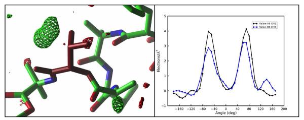
Experimental electron density of the Valine B8 side chain reveals evidence for partial occupancy of the trans rotamer that is preferentially sampled in our simulations. The left-hand panel shows the Fo-Fc map sampled on a 0.50 Å3 grid and contoured at 4.0 (green) and −4.0 (red) in the vicinity of valine B8 (purple). The valine side chain is seen in the experimentally determined gauche(−) rotamer. A region of positive density indicates the missing alternate trans rotamer sampled in our simulation. Image generated with ccp4mg. The right-hand panel shows the output of Ringer⁴⁷ for the χ₁ angle of valine A8 (black) and B8 (blue). An additional peak in the latter case points to the presence of a partially occupied trans rotamer in the electron density.

The coupling between C-terminal helicity and the dry states offers a possible explanation for the sudden shifts in the water diffusivity seen in Figure 6. During the 2.4 μs simulation, after about 400 ns of dynamics, nine of the unit cells in the crystal enter a prolonged one water defect state. The supercell has nine water channels, and dry cell defects are distributed one per channel. Near the end of the trajectory, from 2–2.4 μs, some cells are seen to escape the water defect: with only 6 dry unit cells remaining, water diffusivity increases by almost two fold. These observations indicate that sampling of the one-water-defect corresponds to slowing of the water flow in a given channel. Moreover, two concurrent water defects are very rarely observed in one water channel. We hypothesized that because the water defect corresponds strongly to 3₁₀ helical sampling and because the 3₁₀ helix is a more tightly wound but longer helix, it could be jutting into the channel to sterically impede water movement at that point. Effectively it would serve as a block in the channel which would reduce overall water diffusion. However, expelling waters at the defect site would force them into adjacent cells and inhibit other cells from drying along that particular channel.

4 Conclusions

We present here results of six simulations of a peptide crystal composed of 36 unit cells in a P1 crystal system. Our results offer some of the most detailed agreement to date between a simulation and the diffraction data taken from a biomolecular crystal. In all, the peptide crystal supercell was simulated for 9.6 microseconds. Our results show that the Amber ff99SB force field coupled with a TIP3P water model maintains the integrity of the crystal structure very well. Volume, RMSD and average structure all agree well with experiment. Remarkable B-factor agreement is obtained, except for the final residues of the second peptide. Both the aromatic t-stacking and hydrogen bonding interactions that stabilize crystal packing are maintained. Methodologically, refinement against the average simulation density yields an optimal representation of the average simulation structure and avoids the pitfalls of the more commonly employed coordinate averaging over the simulation trajectory. Calculation of B-factors from coordinate fluctuations yields close agreement with B-factors from crystallographic refinement only when global disorder and lattice distortion effects are accounted for. On the other hand, B-factors from refinement are found to underestimate coordinate fluctuations where the simulation samples an alternate conformation.

The simulation also provided a glimpse into the hidden dynamics of the crystal. The atomic motions seen in the simulation can be placed into three broad categories. Most of the peptide atoms vibrate around a single average structure (with amplitudes well-described by the experimental atomic displacement parameters.) Atoms at the end of the second peptide visit alternate conformations, and the B-factors obtained by refinement against a single structural model underestimate the extent of this motion. (Some evidence for the alternate conformations is present in the observed electron density, but the simulation appears to exaggerate their importance.)

Water molecules observed in the X-ray structure are not bound to any particular unit cell but rather exchange positions frequently within unit cells and between neighboring cells along solvent channels. The timescale of the simulations permits measurements of this diffusion, as well as correlation of protein motion and structural heterogeneity resulting from the migratory crystal defects in unit cells. The dynamic nature of the solvent produces a heterogeneous population of water states with individual unit cells at any given time containing anywhere from zero to eight water molecules. A five-water state is seen to occur most frequently and a fifth lobe of water density is observed corresponding to electron density found in the experimental diffraction data. Somewhat larger defects are also observed in which unit cells dry to only a single water molecule, and these defects appear to slow the diffusion of water throughout entire channels. This transient variability in solvent content offers a reasonable model of the true crystal lattice – the average density of simulated water recovers the crystallographic density with remarkable precision. While traditional crystal refinement to a single ASU gives no indication of water hopping or variation in water content between cells, it is known that mean residence times of single water molecules are short (microseconds even for waters buried deep within a protein cavity^49–51). This behavior is explicitly revealed here by the molecular dynamics simulations. Moreover the simulations lead to the identification of additional water positions and improved refinement statistics (Rwork/Rfree) thus demonstrating the potential utility of all-atom crystal simulations in the interpretation of experimental electron density. We thus provide evidence for the potential of molecular dynamics to contribute additional structural information to the interpretation of crystallographic data that would otherwise remain lost.

An ensemble of two structurally different populations of unit cells is observed. About 25% of the unit cells are characterized by increased 3₁₀ helical propensity, decreased water content (containing only 1 or 2 waters) and occupancy of the gauche(−) χ₁ rotmer of Valine B8. These three characteristics are highly correlated over the course of the microsecond long simulations, but it is unclear which of them might be the driving factor. Because 3₁₀ propensity is not seen in the sequentially identical monomer A, we believe that this behavior is not driven by the valine dihedral but rather must be caused by factors external to the monomer itself. The water channel at the C-terminus provides a spatial opening for the tighter but longer 3₁₀ helix to form, and variations in water content or close contacts with an Aib 5 side chain in monomer A can affect hydrogen bond-stabilizing interactions in the helix. Nevertheless, the presence of this conformational ensemble is only partly consistent with the experimental data, which leads us to believe that part of this observation is a simulation artifact. Careful examination of the experimentally-derived electron density and refinement of a model with an alternate conformation do indeed support the presence of a minor population of the alternate valine rotamer. This is consistent with recent results from the Ringer program⁴⁷, showing that 18% of a test set of pdb structures contained un-identified alternate conformations. As discussed above, the simulated water density also closely tracks the diffraction data. However, the disagreement in B-factors observed in the C-terminus of monomer B indicates that a simulation artifact is present. There is also no substantial evidence in the experimental electron density for the presence of both 3₁₀ and alpha-helical varieties of the second monomer. Thus we conclude, that the observed correlation between the unit cell water content, the Valine B8 rotamer and the helical conformation of the molecule is an artifact of the simulation. This is valuable information for further work on improved force field models for molecular dynamics. A fine equilibrium of protein-protein and protein-solvent interactions drives the formation of the various types of helices⁵², and we suspect that further fine-tuning of hydrogen bond treatment and solvent parameters in current force field models is necessary.^53,54

Thus the development of all-atom crystal simulations requires continued work. More simulations on both small and large structures are needed. We are also continuing investigation of the fav8 peptide with simulations of varying water content as well as simulations using the all-atom AMOEBA^55–57 force field to elucidate the interactions leading to the alternate unit cell population. Taken together, our results demonstrate that molecular dynamics simulations of crystals possess strong potential as both a tool for validating next generation force fields against experimental data and as a powerful tool for extricating additional information about biomolecular structure and dynamics from diffraction data.

References

- [1].Fraser JS, van den Bedem H, Samelson AJ, Lang PT, Holton JM, Echols N, Alber T. Proc. Natl. Acad. Sci. U.S.A. 2011;108:16247–52. doi: 10.1073/pnas.1111325108. [DOI] [PMC free article] [PubMed] [Google Scholar]
- [2].Kruschel D, Zagrovic B. Mol. Biosyst. 2009;5:1606–1616. doi: 10.1039/b917186j. [DOI] [PubMed] [Google Scholar]
- [3].Fraser JS, Jackson C. J. Cell. Mol. Life Sci. 2011;68:1829–41. doi: 10.1007/s00018-010-0611-4. [DOI] [PMC free article] [PubMed] [Google Scholar]
- [4].Burnley BT, Afonine PV, Adams PD, Gros P. eLife. 2012;1:e00311. doi: 10.7554/eLife.00311. [DOI] [PMC free article] [PubMed] [Google Scholar]
- [5].Zagrovic B, Gattin Z, Lau JK-C, Huber M, van Gunsteren WF. Eur. Biophys. J. 2008;37:903–12. doi: 10.1007/s00249-008-0307-y. [DOI] [PubMed] [Google Scholar]
- [6].van Gunsteren WF, Mark AE. J. Chem. Phys. 1998;108:6109. [Google Scholar]
- [7].Showalter SA, Brüschweiler R. J. Chem. Theory. Comput. 2007;3:961–975. doi: 10.1021/ct7000045. [DOI] [PubMed] [Google Scholar]
- [8].Grindon C, Harris S, Evans T, Novik K, Coveney P, Laughton C. Phil. Trans. R. Soc. A. 2004;362:1373–86. doi: 10.1098/rsta.2004.1381. [DOI] [PubMed] [Google Scholar]
- [9].Freddolino PL, Schulten K. Biophys. J. 2009;97:2338–47. doi: 10.1016/j.bpj.2009.08.012. [DOI] [PMC free article] [PubMed] [Google Scholar]
- [10].Nicholls A, Mobley DL, Guthrie JP, Chodera JD, Bayly CI, Cooper MD, Pande VS. J. Med. Chem. 2008;51:769–779. doi: 10.1021/jm070549+. [DOI] [PubMed] [Google Scholar]
- [11].Meinhold L, Smith JC. Proteins. 2007;66:941–53. doi: 10.1002/prot.21246. [DOI] [PubMed] [Google Scholar]
- [12].Schnieders M, Fenn TD, Pande VS, Brunger AT. Acta Crystallogr., Sect. D. 2009;65:952–65. doi: 10.1107/S0907444909022707. [DOI] [PMC free article] [PubMed] [Google Scholar]
- [13].Schnieders M, Fenn TD, Pande VS. J. Chem. Theory. Comput. 2011:110309124812033. doi: 10.1021/ct100506d. [DOI] [PubMed] [Google Scholar]
- [14].Tyka MD, Keedy DA, André I, Dimaio F, Song Y, Richardson DC, Richardson JS, Baker D. J. Mol. Biol. 2011;405:607–18. doi: 10.1016/j.jmb.2010.11.008. [DOI] [PMC free article] [PubMed] [Google Scholar]
- [15].Cerutti DS, Le Trong I, Stenkamp RE, Lybrand TP. Biochemistry. 2008;47:12065–77. doi: 10.1021/bi800894u. [DOI] [PMC free article] [PubMed] [Google Scholar]
- [16].Cerutti DS, Le Trong I, Stenkamp RE, Lybrand TP. J. Phys. Chem. B. 2009;113:6971–85. doi: 10.1021/jp9010372. [DOI] [PMC free article] [PubMed] [Google Scholar]
- [17].Cerutti DS, Freddolino PL, Duke RE, Case DA. J. Phys. Chem. B. 2010;114:12811–24. doi: 10.1021/jp105813j. [DOI] [PMC free article] [PubMed] [Google Scholar]
- [18].Aravinda S, Shamala N, Das C, Sriranjini A, Karle IL, Balaram P. J. Am. Chem. Soc. 2003;125:5308–15. doi: 10.1021/ja0341283. [DOI] [PubMed] [Google Scholar]
- [19].Case D, Darden T, Cheatham T, III, Simmerling C, Wang J, Duke R, Luo R, Walker R, Zhang W, Merz K, Roberts B, Wang B, Hayik S, Roitberg A, Seabra G, Kolossvai I, Wong K, Paesani F, Vanicek J, Liu J, Wu X, Brozel S, Kollman P. University of California; San Francisco: 2010. [Google Scholar]
- [20].Word JM, Lovell SC, Richardson JS, Richardson DC. J. Mol. Biol. 1999;285:1735–47. doi: 10.1006/jmbi.1998.2401. [DOI] [PubMed] [Google Scholar]
- [21].Hornak V, Abel R, Okur A, Strockbine B, Roitberg A, Simmerling C. Proteins. 2006;65:712–725. doi: 10.1002/prot.21123. [DOI] [PMC free article] [PubMed] [Google Scholar]
- [22].Jorgensen WL, Chandrasekhar J, Madura JD, Impey RW, Klein ML. J. Chem. Phys. 1983;79:926. [Google Scholar]
- [23].Wang J, Cieplak P, Kollman PA. J. Comput. Chem. 2000;21:1049–1074. [Google Scholar]
- [24].Berendsen HJC, Postma JPM, van Gunsteren WF, DiNola A, Haak JR. J. Chem. Phys. 1984;81:3684. [Google Scholar]
- [25].Izaguirre JA, Catarello DP, Wozniak JM, Skeel RD. J. Chem. Phys. 2001;114:2090. [Google Scholar]
- [26].Cerutti DS, Duke R, Freddolino PL, Fan H, Lybrand TP. J. Chem. Theory. Comput. 2008;4:1669–1680. doi: 10.1021/ct8002173. [DOI] [PMC free article] [PubMed] [Google Scholar]
- [27].Darden T, York DM, Pedersen L. J. Chem. Phys. 1993;98:10089. [Google Scholar]
- [28].Essmann U, Perera L, Berkowitz ML, Darden T, Lee H, Pedersen LG. J. Chem. Phys. 1995;103:8577–8593. [Google Scholar]
- [29].Ryckaert J, Ciccotti G, Berendsen H. J. Comput. Phys. 1977;23:327–341. [Google Scholar]
- [30].Miyamoto S, Kollman PA. J. Comput. Chem. 1992;13:952–962. [Google Scholar]
- [31].Kabsch W. Acta Crystallogr., Sect. A. 1976;32:922–923. [Google Scholar]
- [32].Kabsch W. Acta Crystallogr., Sect. A. 1978;34:827–828. [Google Scholar]
- [33].Kabsch W, Sander C. Biopolymers. 1983;22:2577–637. doi: 10.1002/bip.360221211. [DOI] [PubMed] [Google Scholar]
- [34].Murshudov GN, Vagin AA, Dodson EJ. Acta Crystallogr., Sect. D. 1997;53:240–55. doi: 10.1107/S0907444996012255. [DOI] [PubMed] [Google Scholar]
- [35].Adams PD, Afonine PV, Bunkóczi G, Chen VB, Davis IW, Echols N, Headd JJ, Hung L-W, Kapral GJ, Grosse-Kunstleve RW, McCoy AJ, Moriarty NW, Oeffner R, Read RJ, Richardson DC, Richardson JS, Terwilliger TC, Zwart PH. Acta Crystallogr., Sect. D. 2010;66:213–21. doi: 10.1107/S0907444909052925. [DOI] [PMC free article] [PubMed] [Google Scholar]
- [36].Afonine PV, Grosse-Kunstleve RW, Echols N, Headd JJ, Moriarty NW, Mustyakimov M, Terwilliger TC, Urzhumtsev A, Zwart PH, Adams PD. Acta Crystallogr., Sect. D. 2012;68:352–67. doi: 10.1107/S0907444912001308. [DOI] [PMC free article] [PubMed] [Google Scholar]
- [37].Humphrey W. J. Mol. Graph. 1996;14:33–38. doi: 10.1016/0263-7855(96)00018-5. [DOI] [PubMed] [Google Scholar]
- [38].McNicholas S, Potterton E, Wilson KS, Noble MEM. Acta Crystallogr., Sect. D. 2011;67:386–94. doi: 10.1107/S0907444911007281. [DOI] [PMC free article] [PubMed] [Google Scholar]
- [39].Winn MD, Ballard CC, Cowtan KD, Dodson EJ, Emsley P, Evans PR, Keegan RM, Krissinel EB, Leslie AGW, McCoy A, McNicholas SJ, Murshudov GN, Pannu NS, Potterton EA, Powell HR, Read RJ, Vagin A, Wilson KS. Acta Crystallogr., Sect. D. 2011;67:235–42. doi: 10.1107/S0907444910045749. [DOI] [PMC free article] [PubMed] [Google Scholar]
- [40].Agarwal RC. Acta Crystallogr., Sect. A. 1978;34:791–809. [Google Scholar]
- [41].Maslen EN, Fox AG, O'Keefe MA. International Tables for Crystallography, Vol C, Mathematical, Physical and Chemical Tables, Table 6.1.1.4 Coefficients for analytical approximation to scattering factors. 2nd ed. Kluwer Academic Publishers; Dordrecht: 1999. Intensity of diffracted intensities. [Google Scholar]
- [42].Howell PL, Smith GD. J Appl Crystallogr. 1992;25:81–86. [Google Scholar]
- [43].Brünger AT. Acta Crystallogr., Sect. D. 1993;49:24–36. doi: 10.1107/S0907444992007352. [DOI] [PubMed] [Google Scholar]
- [44].Kleywegt GJ. Acta Crystallogr., Sect. D. 2007;63:939–40. doi: 10.1107/S0907444907033458. [DOI] [PubMed] [Google Scholar]
- [45].Cruickshank DWJ. Acta Crystallogr. 1956;9:747–753. [Google Scholar]
- [46].Baez LA, Clancy P. J. Chem. Phys. 1994;101:9837. [Google Scholar]
- [47].Lang PT, Ng H-L, Fraser JS, Corn JE, Echols N, Sales M, Holton JM, Alber T. Protein Sci. 2010;19:1420–31. doi: 10.1002/pro.423. [DOI] [PMC free article] [PubMed] [Google Scholar]
- [48].Scouras AD, Daggett V. Protein Sci. 2011;20:341–52. doi: 10.1002/pro.565. [DOI] [PMC free article] [PubMed] [Google Scholar]
- [49].Modig K, Liepinsh E, Otting G, Halle B. J. Am. Chem. Soc. 2004;126:102–114. doi: 10.1021/ja038325d. [DOI] [PubMed] [Google Scholar]
- [50].Halle B. J. Chem. Phys. 2003;119:12372–12385. [Google Scholar]
- [51].Lesage A, Lyndon E, Penin F, Böckmann A. J. Am. Chem. Soc. 2006;128(25):8246–8255. doi: 10.1021/ja060866q. [DOI] [PubMed] [Google Scholar]
- [52].Dill KA. Biochemistry. 1990;29:7133–7155. doi: 10.1021/bi00483a001. [DOI] [PubMed] [Google Scholar]
- [53].Lange OF, van der Spoel D, de Groot BL. Biophys. J. 2010;99:647–655. doi: 10.1016/j.bpj.2010.04.062. [DOI] [PMC free article] [PubMed] [Google Scholar]
- [54].Kortemme T, Morozov AV, Baker D. J. Mol. Biol. 2003;326:1239–1259. doi: 10.1016/s0022-2836(03)00021-4. [DOI] [PubMed] [Google Scholar]
- [55].Ponder JW, Wu C, Ren P, Pande VS, Chodera JD, Schnieders M, Haque I, Mobley DL, Lambrecht DS, DiStasio RA, Head-Gordon M, Clark GNI, Johnson ME, Head-Gordon T. J. Phys. Chem. B. 2010;114:2549–64. doi: 10.1021/jp910674d. [DOI] [PMC free article] [PubMed] [Google Scholar]
- [56].Ren P, Ponder JW. J. Phys. Chem. B. 2003;107:5933–5947. [Google Scholar]
- [57].Ren P, Wu C, Ponder JW. J. Chem. Theory. Comput. 2011;7:3143–3161. doi: 10.1021/ct200304d. [DOI] [PMC free article] [PubMed] [Google Scholar]
Associated Data
This section collects any data citations, data availability statements, or supplementary materials included in this article.