Abstract
Precopulatory sexual selection is the association between fitness and traits associated with mate acquisition. While sexual selection is generally recognized to be a powerful evolutionary force, most investigations are limited to characters belonging to individuals. A broader multi-level perspective acknowledges that individual fitness can be affected by aspects of mating success that are characters of groups, such as families. Parental mating success in polygynous or polyandrous human societies may exemplify traits under group-level sexual selection. Using fitness measures that account for age-structure, I measure multi-level selection for mate number over 55 years in a human population with declining rates of polygyny. Sexual selection had three components: individual-level selection for ever-mating (whether or not an individual mated) and individual- and family-level selection for polyandry and polygyny. Family- and individual-level selection for polygyny was equally strong, three times stronger than family-level selection for polyandry and more than an order of magnitude stronger than individual-level selection for polyandry. However, individual-level selection for polyandry and polygyny was more effective at explaining relative fitness variance than family-level selection. Selection for ever-mating was the most important source of sexual selection for fitness; variation for ever-mating explained 23% of relative fitness variance.
Introduction
Competition among individuals for reproductive partners causes variation for fitness, a necessary condition for evolution by natural selection. This component of fitness variance, sexual selection, has long been believed to be an important agent of evolutionary change (Darwin 1871). The strength of sexual selection in a population follows from its mating system. High rates of polygyny, for example, should generate more sexual selection (Clutton-Brock et al. 1977; Wade 1979; Wade and Shuster 2004b). Comparative studies support this expectation (Bateman 1948; Lofredo and Borgia 1986; Andersson 1994; Jones and Avise 2001; Shuster and Wade 2003; Moorad et al. 2011), but much interest remains in measuring the strength of sexual selection and understanding its quantitative role in the evolution of phenotypes (Arnold and Duval 1994; Jones 2009; Krakauer et al. 2011).
There are at least two statistical frameworks for understanding the role of selection in evolutionary change, and sexual selection is measured in terms of both. The first measures selection gradients, or the slope of relative fitness (a mean-standardized measure of fitness) on individuals' trait values (Robertson 1966; Price 1970; Lande and Arnold 1983). When multiplied by the heritable genetic trait variances, selection gradients define evolutionary responses to selection over a single generation. A trait can contribute to fitness through associations with mating success, or by some other means (e.g., survival or per-mate fertility), but it is only through generating mating success variation that a trait can be said to be under precopulatory sexual selection. While the strength of associations between trait values and mating success are trait-specific, the associations between mating success and fitness are not (although these associations are likely to be sex-specific). The strength of these key associations are quantified as slopes of fitness on mating success, or `Bateman gradients' (Arnold and Duval 1994; Jones 2009). These are highly useful measures as they place an upper bound on the potential of precopulatory sexual selection to cause evolutionary change in trait values (for the remainder of this paper, sexual selection is understood to mean precopulatory sexual selection).
A second measure of selection is the relative fitness variance or I, the `opportunity for selection' (Crow 1958; O'Donald 1970a, b; Wade 1979; Wade and Arnold 1980). The product of I and narrow-sense fitness heritability defines the improvement in mean fitness caused by natural selection over one generation. This measure of the short-term adaptive potential of a population is considered a highly useful measure for comparing selection across populations (Hersch and Phillips 2004; Walsh and Lynch 2008). This concept has been extended to that portion of the total fitness variance that is attributable to variation in mating success, Is, the opportunity for sexual selection (Arnold and Wade 1984; Wade 1995; Shuster and Wade 2003; Moorad and Wade 2013). Sex-specific Bateman gradients, opportunities for selection, and opportunities for sexual selection have been measured in many culturally and temporally distinct human populations (Brown et al. 2009; Moorad et al. 2011; Courtiol et al. 2012). Recently Moorad and Wade (2013) showed how these measures are inter-related. While great variation among sexual selection measurements exists among these populations, strong evidence suggests that sexual selection is stronger in males than in females and this divergence is strengthened in populations with high rates of polygyny.
Despite the popularity of these sexual selection measures, there are at least two potential problems associated with interpreting Bateman gradients and opportunities for selection. The first is the problem of what to do about intergenerational effects. In particular, how is selection to be quantified if an individual's fitness is sensitive to the number of mates its father (or mother) had? This issue is occasionally addressed in human studies by changing the definition of fitness from the number of offspring produced to the number of grandchildren produced (e.g., Josephson 1993; Hill et al. 1995; Mace 1998; Gillespie et al. 2008). Regressions of this two-generation measure of fitness on mating success yield associations that incorporate the intergenerational effects. Unfortunately, these regressions obfuscate signatures of inter-generational evolutionary dynamics, such as conflict or cooperation, that are resolvable with more sophisticated approaches designed to measure selection for parental effects (Falconer 1965; Cheverud 1984; Cheverud and Moore 1994; Wade 1998; Wolf and Brodie 1998; Bijma and Wade 2008; McGlothlin et al. 2010).
A second problem involves the meaning of fitness when populations are age-structured. The need to incorporate age-structure into measurements of sexual selection was recognized recently by Jones (2009). When generations do not overlap, or if the size of the population stays constant over time, then relative fitness is simply the number of offspring produced (absolute fitness) divided by the mean reproductive output of the population (Caswell 2001). In other situations, such as expanding human populations (e.g., Hamilton 1966; Moorad et al. 2011), individual fitness is more complicated because the relationship between fitness and fertility depends upon the timing of reproduction and the growth rate of the population (Fisher 1958). When reproductive timing is ignored in growing populations, selection for early-acting traits is underestimated, and selection for late-acting traits is overestimated (e.g., Moorad 2013). For a trait such as mating success, where the value is taken as cumulative count of mates of the lifetime of the individual, ignoring age-structure will cause one to mis-measure sexual selection. This problem is exacerbated if the number of grandchildren is used for fitness because the variance in the timing of grandchild production is greater than the variance in timing of offspring production.
The current study measures sexual selection in a human population. The multi-level approach taken here addresses intergenerational effects by quantifying separately selection operating on mating success through the individual and through the parents. I apply contextual analysis (Heisler and Damuth 1987; Damuth and Heisler 1988; Goodnight et al. 1992; Okasha 2004), a regression-based approach intended to provide multi-level selection gradients that are interpretable in the Lande-Arnold multivariate selection framework (Lande and Arnold 1983), to measure selection for six specific traits related to mating success. These traits are:
-
1 – 2)
selection for ever-mating in males and females (whether or not individuals of a specific sex successfully mated at least once);
-
3)
individual-level selection for male polygyny (if a male reproduced, how many females did he reproduce with);
-
4)
individual-level selection for female polyandry (if a female reproduced, how many males did she reproduce with); and
-
5 – 6)
family-level selection acting on the sire polygyny and dam polyandry (how many reproductive partners did the individual's father and mother have).
This refined perspective yields novel, multi-level `Bateman gradients' that quantify how mating system affects fitness when intergeneration interactions are present.
The study population is a large collection of individuals who immigrated to, or were born in, what is now the state of Utah in the Western United States. Individuals studied here were born in the 19th century over a 55-year period that saw a transition of marriage practices from a time when polygamy was common to a later time when it was not (Smith and Kunz 1976; Moorad et al. 2011). I define polygynists as men who reproduce with two or more women at any point in their lives; these include polygamists and monogamists who have remarried after a divorce or a death of a wife. Polyandrists are always remarried women. This population experienced high growth rates, with individuals from some birth year cohorts averaging family sizes of over six children (Moorad et al. 2011). Following Moorad (2013), I define fitness as the reproductive value at birth. However, I generalize the measure to allow for sex-specific survival and reproductive rates (see Appendix). This refined definition of individual fitness is more appropriate for regression-based studies of sexual selection in age-structured populations.
Methods
The model
Contextual analysis (Heisler and Damuth 1987) views fitness as a property of the individual, but it allows fitness to be explained by traits that are properties of the individual or the group (contextual traits). Contextual traits are often defined as the trait means of the entire group (e.g., Goodnight et al. 1992) or the means of the group that exclude the focal individual (e.g., Bijma et al. 2007). Maternal (or paternal) traits are an extreme application of the latter because the group effect is derived from single individuals (the mother or father). The sex-specific parental effects are nonetheless contextual because they define properties of the group: the maternal (or paternal) effect upon the fitness of their children. For my analysis of multi-level sexual selection, I define individual fitness as a linear model of individual and family-level traits defined in Table 1,
| (1). |
Five of these predictor traits are unconditional because they are expressed by all individuals; these include three individual-level traits (survival to age 15, sex, and sex-by-survival interactions) and two contextual traits, sire polygyny (Gsire,i) and dam polyandry (Adam,i). Four conditional traits describe the mating success of the individual. Expression of these traits requires survival to age 15 and belonging to a specific sex. In addition, individual multiple-mating requires ever-mating. When these conditions are not met (an individual is not capable of mating if it dies in infancy, for example), trait values are imputed following the method of Moorad and Wade (2013) discussed in the next section. Note that (1) accounts for all fitness effects of mate number, including the differences caused by non-reproductive individuals.
Table 1.
| Symbol | Definition | Property of the … |
|---|---|---|
| wi | Relative fitness | individual |
| μ | Mean relative fitness (equal to 1) | individual |
| Li | Survival to age 15 (0 or 1) | individual |
| Si | Sex (1 for male and 0 for female) | individual |
| I(L×S)i | Interaction between sex and survival | individual |
| Mi|(L, S = l) | Ever-mated male (1 if he reproduced and 0 if he did not) conditional on survival and being male. | individual |
| Fi|(L, S = 1,0) | Ever-mated female (1 if she reproduced and 0 if she did not) conditional on survival and being female. | individual |
| Gi|(L, S, D = l) | Individual polygyny (number of unique reproductive partners) conditional on survival, being male, and male ever-mated | individual |
| Ai|(L, S, D = 1,0,1) | Individual polygyny (number of unique reproductive partners) conditional on survival, being female, and mating at least once | individual |
| Gsire,i | Sire polygyny | family |
| Adam,i | Dam polyandry | family |
| ε i | Residual error | individual |
Conditional traits
I invoke conditional traits for two reasons. First, comparisons between the relative strength of individual vs. group level selection are best interpreted if individual and contextual traits have clear statistical relationships (e.g., when the contextual trait is the group-mean phenotype, such as in Goodnight et al (1992)). While mate number (mating success) is often the trait of interest in sexual selection studies, distributions of individual and parental mating success are fundamentally different because individuals frequently fail to reproduce and all parents, by definition, have at least one reproductive partner. By conditioning individual, sex-specific mating success upon survival to age 15 (no parent born prior to 1900 in the UPDB dies before reaching this age) and on ever-mating, the meanings of individual and parental polygyny/polyandry converge. Thus, easily interpretable comparisons can be made between the strength of selection for multiple-mating acting at two levels (βwG,βwA and βwGsire,βwAdam, respectively). This model constrains all selection for ever-mating (βwM, βwF) to act at the level of the individual.
Second, conditional traits enhance the causal model of fitness by discriminating between viability and mating success. Sexual selection is frequently quantified by the strength of the association between fitness and number of mates (Bateman 1948; Arnold and Duval 1994; Shuster and Wade 2003; Jones 2009). However, viability selection risks being confounded with sexual selection if mortality precedes reproductive maturity. Using a subset of the population analyzed here, Moorad and Wade (2013) accounted for juvenile mortality in a phenotypic selection model of sexual selection by generalizing the causal model of relative fitness to include survival to age 15 and by conditioning sex-specific mating success upon survival and sex. Trait values that were precluded by mortality or by sex (e.g., female mating success in males) were imputed with the trait means of the subset of the population with data that existed. For example, male ever-mating in females and males that died prior to age 15 was the mating frequency of males that survived to 15.
This imputation strategy has three consequences. First, all individuals have all traits, and the intra-trait phenotypic correlation matrix is assured to be invertible. This is a necessary condition for multivariate phenotypic selection analyses (Lande and Arnold 1983). Second, selection gradients are unaffected by the expressed fraction (the proportion of the population that satisfies the conditions). The phenotypic variance of the population, however, is the product of the expressed fraction and the expressed variance (the trait variance of the population subset that expresses the trait). For example, if one-quarter of the population was female, lived to be 15, and reproduced at least once, then the population's individual polyandry variance would be 25% of the expressed variance. In the companion paper, Moorad (2013) used this approach to estimate the strength of selection for female vital rates (age-specific survival and fertility) in the Utah population. Vital rates were conditional on cumulative survival. Selection gradients for vital rates estimated in this way agreed with estimates obtained from conventional life-history approaches that do not use multiple regressions (Hamilton 1966; Charlesworth 1994; Caswell 2001). Third, conditional traits are orthogonal to the traits upon which they are conditioned. Thus, there are no correlations between M,F,G, A and L, S, I(L×S) nor between M,F and G, A. However, conditional individual traits M,F,G, A and unconditional family-level traits Gsire, Adam may be correlated; such correlations arise from heritable genetic variation and covariation and from indirect genetic effects that contribute to a response to selection only by shaping patterns of trait inheritance (Bijma and Wade 2008). The multivariate regression-based approach employed by contextual analysis ensures that these correlations do not affect phenotypic selection estimates.
The Utah Population Database
I used two sets of data from the Utah Population Database (UPDB) that were kindly provided by Dr. Ken Smith of the University of Utah. The first set contained birth and death years of 62,756 unique reproductive females (`females') and 65,561 unique reproductive males (`males') born between 1840 and 1894. The second set contained birth years, sex, and parental identification for 630,410 individuals (children). From the second set, a subset was defined that contained birth years and maternal identification for 299,572 females (daughters) and 313,962 males (sons) born between 1840 and 1970. These sets were not exclusive, nor did inclusion in the second set necessarily mean that a given individual was a child of an individual from the first set. Using the `females', `males', `daughters', and `sons' datasets, individual records for all individuals born between 1840 and 1894 were constructed with: 1) years of birth, death, and production of any sons and daughters; 2) sex; and 3) the number of mates (unique reproductive partners) attributed to the individual, its mother, and its father. Individuals were subdivided into 55 birth-year-specific populations (cohorts) and treated as independent populations. The number of individuals belonging to each cohort increased with increased birth year beginning with 1917 in 1840 and increasing to 8650 in 1894 (Figure A1). Further details, including the method used to estimate the size and composition of the non-reproductive class of individuals, can be found in the Appendix.
The linear model (1) includes sire polygyny and dam polyandry measures that were occasionally unavailable because parents were not identified. The frequency of missing data for either parent was high (41%) in the earliest birth year cohorts, but this fraction quickly decreased to 7.3% by the end of the study period (Figure A1). Parent data was not missing completely at random; for example, there was greater fitness variance among individuals with complete parent information. This suggested two possible data analyses. Model 1 considered all individual traits in (1) and all available individuals, but it neglected multiple-mating in parents. Model 2 included parental mating, but ignored individuals with missing parent records. Parental mating may correlate with the conditioning individual traits (sex, survival, and sex-by-survival interactions). High maternal mate number might compromise offspring survival, for example. Conditional traits are not included in Model 2 to allow estimates of family-level selection for multiple-mating to include indirect effects on fitness through offspring sex, survival, or sex-by-survival interactions (traits that are always independent of individual ever-mating and multiple-mating).
Two possibilities may explain why the approaches might yield different measures of selection. Complete and incomplete populations might exhibit different relationships between traits and fitness. Alternatively, parental multiple-mating may be an important determinant of fitness and correlate with individual multiple-mating. If so, selection gradients for individual and family-level multiple-mating would be difficult to reconcile across the two analyses. However, there was good evidence to suggest that the correlational effects were minimal (see Results), and a multi-level perspective of selection for multiple-mating could be synthesized from family-level selection gradients obtained from Model 2 and individual-level selection gradients obtained from Model 1.
Measuring selection
I defined individual fitness using individual reproductive values at birth (see Appendix). For each birth year cohort, I applied a multiple regression of this measure on the trait values defined in (1). Selection gradients were estimated from partial least-squared regression coefficients using the `lm' function in R 2.11.0 (R Development Core Team 2011). Gradients were estimated independently for Models 1 and 2. I do not report selection gradients for conditional traits. The strength of selection for specific traits was the product of gradients and trait variances, measured directly from the imputed data. Recall that this variance reflects the proportion of the population that expresses the trait and that all individuals express the parental mating traits.
The total opportunity for selection I is the relative fitness variance among individuals. Moorad and Wade (2013) demonstrated how I can be decomposed into orthogonal components attributable to specific traits. Given a causal model of relative fitness w(z), such as that defined in (1), the relative fitness variance attributable to any trait z is equal to βwzbwzq var (z), where βwz is the partial regression coefficient of relative fitness on the trait (the selection gradient), bwz is the simple regression coefficient, q is the expressed fraction, and var(z) is the expressed variance. The product bwz qvar(z) is the selection coefficient. I report contributions to I that are attributable to individual ever-mating and multiple-mating in individuals and parents. I also report the pooled contribution from the conditioning traits.
Selection measures (and their determinants) are presented as functions of cohort birth year. Significance is assessed by bootstrap resampling (R = 10,000) over the cohort measures using the `boot' function (Davison and Hinkley 1997; Canty and Ripley 2012) in R 2.11.0. Significant linear and quadratic relationships between measures and birth year are assessed by polynomial regression (z=b0+b1(byr−1867)+b2(byr−1867)2ε), where 1867 is the mid-point of the study period. Regression coefficients are resampled over 10,000 iterations. Estimates, 95% bias-corrected confidence intervals, and p-values for means, linear time-trends, and quadratic time-trends are compiled in Table A1 in the Appendix.
Results
Nearly all measures and linear time trends departed from zero at a level of significance of p < 0.0001. In the discussion of results that follows, it is understood that this level of significance applies unless another value is given.
Demographic Trends
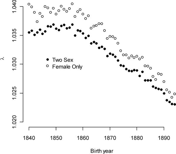
The study period clearly captured a key component of a demographic transition. The intrinsic population growth rates (Figure 1) exceeded one in every year throughout the study period (the average growth rate over all cohorts was 1.032). Growth rates decreased over time (0.000258/year), however, and this decrease accelerated over time (βλt2=−5.13×10⁻⁶). This pattern reflects the secular trend reflected by a female-only analysis of the same Utah population (Moorad 2013). The population growth rates calculated here appeared to be slightly less than in the female-only population, and the range in growth rate values seemed to be suppressed. Both differences make qualitative sense. The expected reproductive output of females at birth must be greater than that of males because the sex ratio at birth is slightly biased towards males. In such situations, we expect that a hypothetical female-only population would appear to grow faster than a two-sex population. Furthermore, one would expect that males dampened short-term fluctuations in population growth rates because they had a longer reproductive tenure than females (Moorad et al. 2011).
Figure 1.
Intrinsic population growth rates decreased over time. Dark circles indicate intrinsic population growth rate for each birth year cohort using the two-sex model. Open circles indicate intrinsic population growth rates for the female-only population, as estimated by Moorad (2013).
Rates of multiple-mating
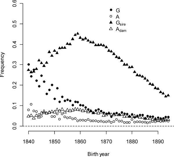
The study period also captured a mating system transition. The rate of multiple-mating for individuals decreased for both sexes. Multiple-mating is used here to indicate polygyny or polyandry, depending upon the sex of the focal individual. The average polygyny rate over the study period was 10.2%, but initial rates were far higher (Figure 2): the earliest rates were approximately 30%, and frequencies fell an average of 0.379% per year. Most of the declines occurred early (βλt2=1.17×10⁻⁴). Part of this pattern was owing to a dramatic decrease in rates of polygamy from approximately 10% of married men in the early birth-year cohorts to 0% by the 1860s (Moorad et al. 2011). Very high male fertility over these years, even in monogamous men, required long reproductive tenures often enabled by widowed or divorced men fathering children with second or third wives. Whatever caused the fertility transition may have reduced the frequency of reproductive second marriages and contributed to declining polygyny rates.
Figure 2.
Rates of polygyny and polyandry in individuals (G and A) and in their parents (Gsire and Adam) changed with time.
Rates of female polyandry were lower than polygyny, beginning at 7.9% in 1840 and averaging 3.47% over the study period. Polyandry rates declined by 0.0978%/year, likely because females ceased reproducing at earlier ages and either reduced the frequencies of reproduction with second husbands or reduced the remarriage frequency. Rates of paternal polygyny were very high: the average fraction of individuals with a father with more than one reproductive partner was 32.0%. This fraction reached a maximum of 45.2 % for individuals born in 1859 before declining to 14.9% at the end of the study period (βG(sire)t=−3.08×10⁻³,βG(sire)t2=−2.91×10⁻⁴. The highest rates of paternal polygyny (1855–1870) occurred 25–40 years after individual polygamy rates peaked (Moorad et al. 2011); this lag corresponds approximately to a generation time extended by polygamy in the Utah population (Bean and Mineau 1986). Dam polyandry rates were low throughout the study (averaging 5.62%), beginning at 4.8%, increasing to 8.2% in 1859, and then declining to 3.2% by 1894 (βA(dam)t=−6.57×10⁻⁴,βA(dam)t2=−4.22×10⁻⁵).
Selection for ever-mating
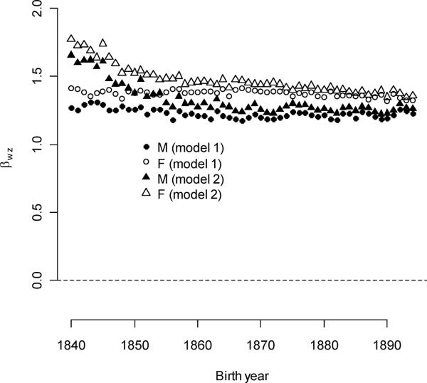
As all parents mate, ever-mating for parents is invariant, and all selection for ever-mating must act at the level of the individual. Male and female selection gradients were estimated for each birth cohort; these are equivalent to the mean relative fitness of reproducing adults. Selection gradients were very high and depended upon sex and the regression model (Model 1 vs. Model 2). From Model 1 (ignoring parental mating), male selection gradients averaged 1.23 and declined slightly by 0.00120/year (Figure 3A). Female gradients exceeded male gradients, , and they also declined slightly by 0.00086/year. From Model 2 (ignoring individuals without identified parents), selection gradients for both sexes were higher than in Model 1 (,), and they declined more steeply (0.00576/year and 0.00572/year, respectively). Both declines slowed over time (ββ(wM)t2=2.70×10⁻⁴,ββ(wF)t2=−1.58×10⁻⁴).
Figure 3A.
Selection gradients for ever-mating in females (open circles and triangles) exceeded those for males (closed circles and triangles).
There are two possible reasons for the differences between Model 1 and Model 2 results. First, partial regression coefficients βwM and βwF reflect correlations with the parental multiple-mating traits in the Model 2 analysis because the effects of these contextual traits are not partitioned out. Because both models constrain individual-level multiple-mating to be independent of ever-mating, the degree to which the inclusion of family-level traits alters the estimation of βwM and βwF can be assessed by comparing these partial regression coefficients with the simple regression coefficients, bwM and bwF. These values proved to be highly similar: over the entire study period, βwM : bwM ranged from 0.987 to 1.002 and βwF :bwF ranged from 0.990 to 1.003 (see Figure A2 in the Appendix). This strongly suggests that the regression structure of Model 2 did not cause the estimated partial regression coefficients to diverge from the selection gradients estimated using Model 1. Instead, it appears that the differences were caused by non-random sampling of the Model 2 population from the complete population of individuals. I present only the results from the Model 1 analysis in this report and discussion of individual trait selection. I use results from Model 2 in my analysis of selection for family-level traits.
Higher selection gradients for ever-mating in females is consistent with an earlier observation from these data that females had slightly more children than males born in the same year (Moorad et al. 2011). This may have been the result of sex-differences in the age at marriage as females in this population typically paired with older males. As a result, males experienced the dramatic fertility transition of this period before the females of the same age. Furthermore, age structure may exaggerate the fitness consequence of this phenomenon because rapidly growing populations place a large fitness premium on early reproduction (Fisher 1958; Hamilton 1966; Caswell 2001). One might expect that slightly male-biased sex ratios at birth would have contributed to the higher selection gradients in females. It should be remembered, however, that ever-mating was conditional upon survival to age 15. As this fraction was smaller in males than in females, the operational sex ratio was more equitable than the sex ratio at birth (see Fig 4 and discussion below). In fact, relatively high childhood mortality in males during the early part of the study was sufficient to cause the operational sex ratio to be female-biased, which should have reduced the selection gradient differences. Operational sex rations in the later years (after 1860) favored males slightly, and this may have contributed to these differences in ever-mating selection gradients.
Figure 4.
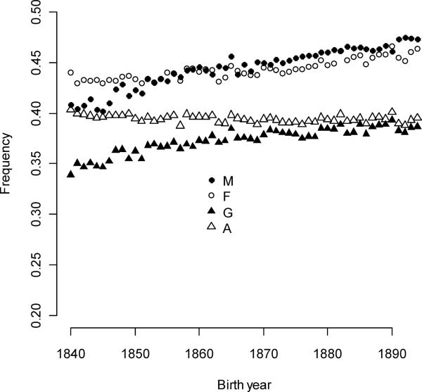
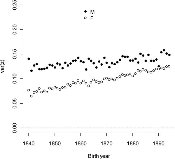
Trait variance in expressed individuals increased for male ever-mating and polygyny and, to a lesser degree, for female ever-mating. The polyandry expression variance decreased slightly over the study period.
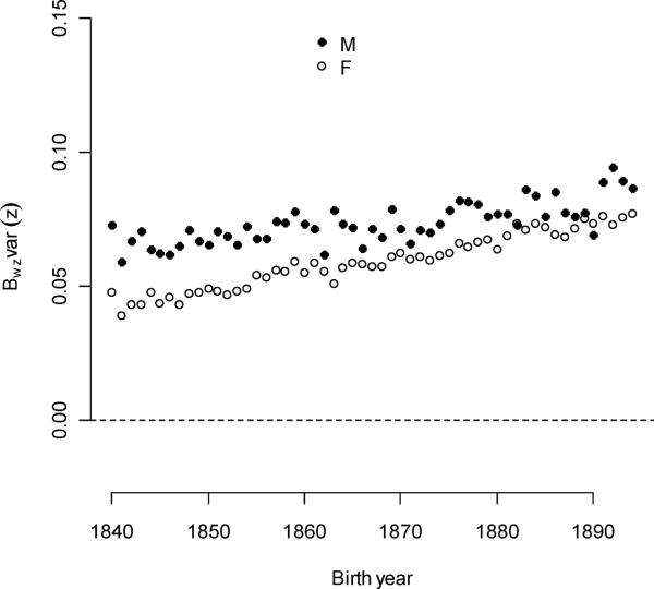
The strength of selection for a trait (or, more simply, selection) is the product of the selection gradient, the fraction of the population that exhibits the trait (the expressed fraction), and the trait variance among individuals belonging to this fraction (the expressed variance). For ever-mating, the conditions for expression are sex and survival to the age of 15 years. For males, the mean expressed fraction for ever-mating was 44.5%, with an annual increase of 0.119% per year (Figure 4). Fractions for females were similar (44.3%), but their secular trend was relatively muted (+5.30×10⁻⁴% per year). Improving juvenile survival (Bean et al. 2002) caused these increases. Expressed variances for ever-mating was always higher in males and increased in both sexes, but sex-differences became smaller with time (Figure 5a). The strength of selection for male ever-mating was greater than selection for female ever-mating, owing largely to its greater expressed variance and despite its smaller selection gradients. Averaged over all birth year cohorts, selection for male ever-mating was 24.5% stronger than selection for female ever-mating, but this advantage declined over time from its maximum of 52.6% in 1840 (Figure 6a).
Figure 5A.
Sex-specific expression variances for ever-mating increased with birth year.
Figure 6A.
The strength of selection for ever-mating in both sexes increased with birth year.
Individual-level selection for multiple-mating
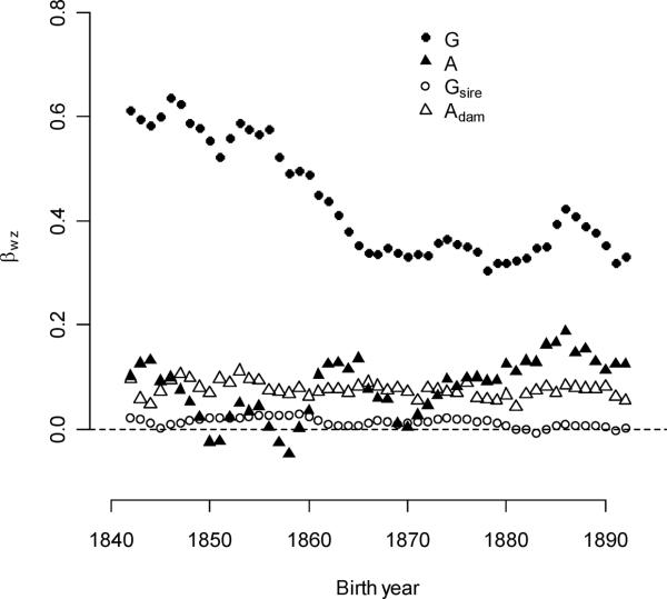
Individual-level selection gradients for multiple-mating were much higher for males than for females (Figure 3b). Averaged over all birth years, these were 0.440 and 0.0827, respectively. Selection gradients for individual polygyny decreased by 0.00646/year over the entire study period. The decline slowed over time (ββ(wG)t2 =1.76×10⁻⁴), and most of the decline was coincident with the decline of individual polygyny in the first twenty years. Note that declining selection gradients do not directly reflect changes in the rate of polygyny; instead, they reflect changes in the fitness consequence of polygyny. Selection gradients for polygyny exceeded those for polyandry in every birth cohort, although differences appeared to be smallest after the abandonment of polygamy. Selection gradients for individual polyandry increased by 0.00164/year.
Figure 3B.
Selection gradients for individual polygyny declined over the study period. These exceeded selection gradients for other multiple-mating traits. Values represent five-year moving averages.
Expression of individual polygyny and polyandry are conditional upon sex-specific ever-mating (which were conditional, in turn, upon survival and sex). The expressed fraction for polygyny selection (mean = 37.3%) increased 0.0731%/year but at rates less than expected by increases in survival alone (equal to the expressed male ever-mating fraction, which increased 0.119%/year). Differently put, surviving males were less likely to mate, or mated males were less likely to reproduce. Similarly, female survival frequencies increased over the study period, but these changes did not translate into expressed fractions of polyandry (+0.0530%/year female ever-mating fraction and −0.00910%/year polyandry fraction). A greater fraction of individuals became a mother than became a father in every birth year cohort, although the difference between sexes declined. Expressed polygyny variance was initially high, but these values fell (the average variance was 0.100 and the annual decline was 0.00372/year – see Figure 5b). Expressed polyandry variances were lower than expressed polygyny variances, and these also decreased with time (the average variance was 0.0343 and the annual decline was 0.0009/year).
Figure 5B.
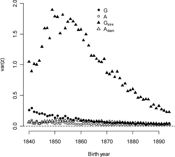
Expression variances for parental multiple mating exceeded variances for individual multiple mating in both sexes.
Family-level selection for multiple-mating
Compared with individual polygyny, parental polygyny and polyandry produced a very slight benefit to offspring fitness (Figure 3b). Selection gradients for paternal polygyny were less than one-thirtieth those for individual polygyny (the mean gradient was 0.0127, compared to 0.440 for the individual trait), and the paternal gradient also declined with time (−0.0004/year, p = 0.0064). Selection gradients for maternal polyandry were roughly equitable to those of individual polyandry values (the mean gradient was 0.0775, compared to 0.0817 for the individual trait), but unlike the individual selection gradients, the gradient for dam polyandry did not change significantly with birth year (p = 0.1505).
As every individual had a father and a mother, the expressed fraction for both parental multiple-mating traits was one. Expressed sire polygyny variance was an order of magnitude greater than expressed individual polygyny variance (the mean sire value over all cohorts was 1.01 compared to 0.100 for individuals - see Figure 5). Expressed sire variance decreased quickly over the entire study period by −0.0266/year, but reached an intermediate maximum in the late 1840s and early 1850s (βvar(Gsire)t2 =−7.74×10⁻⁴). At its maximum in 1849, the sire polygyny variance was 10.3 times greater that the expressed individual polygyny variance. In the first five years (1840–1845) the ratio was three to five times greater. Birth years cohorts of 1845–1865 had rapidly dwindling frequencies of polygamous marriages, but their fathers were born at times corresponding to the greatest frequencies of polygamous marriages. This lag explains a small part of the relative difference between sire and individual polygyny variance, but a more important cause was that polygynous men produced more children than monogynous men (Moorad et al. 2011). As a result, extremely successful males are more heavily weighted in the distribution of sire polygyny than in the distribution of individual polygyny. As the former distribution is often heavily right-skewed (Shuster and Wade 2003), the means and variances of the sire polygyny distributions are amplified relative to the expressed individual distributions. A similar phenomenon occurs for dam polyandry variance, which here was usually an order of magnitude smaller than sire polygyny variance but usually one to three times higher than individual polyandry variance.
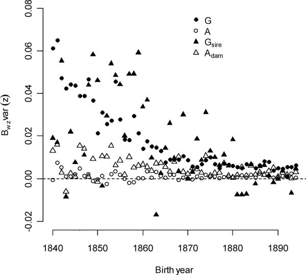
Averaged over all birth-year cohorts, individual-level polygyny selection was not significantly stronger than family-level polygyny selection (0.0185 vs. 0.0158, p = 0.1749 – see Figure 6b). Selection gradients for sire polygyny were much lower (Figure 3b), but higher expressions fractions and expression variances for sire polygyny compensated for this difference. The strength of selection from both sources declined over time (−0.00088/year and −0.00061/year, respectively), but the difference in rates of changes was not significant (p = 0.0634). Multi-level polyandry selection was much weaker than these components of selection, but it was stronger than polyandry selection acting through individuals (0.00512 vs. 0.00107, p < 0.0001). While multi-level selection gradients for polyandry were equitable (no significant difference, p = 0.3889), high expressed fractions and variance in mothers caused family-level selection to be approximately four times stronger. Individual selection for polyandry did not change significantly over time (p = 0.1990), but selection for polyandry through the dam declined with increased birth year (−0.00011/year, p = 0.0062).
Figure 6B.
The strength of selection for male mating traits was greater than that for females. Family- and individual-level selection for polygyny were equally strong, and both declined over time. Family-level selection for polyandry exceeded individual-level selection.
Opportunity for selection and its components
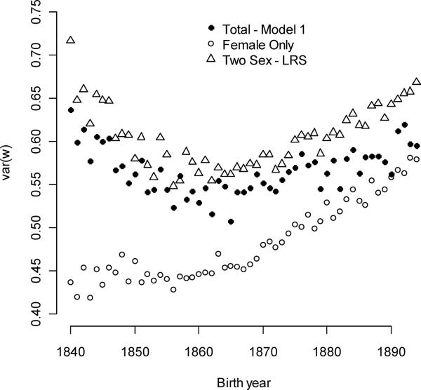
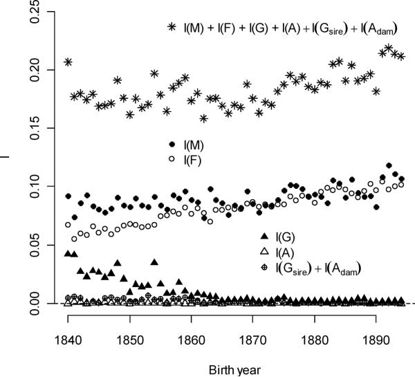
The opportunity for selection, I, averaged 0.567 and was a convex function of birth year, with a minimum of 0.533 in 1865 (Figure 7). Components of I derived from traits identified in the fitness model (1) also changed with time. The component that followed from the combination of directional selection for all individual and family-level mating traits (mean of 0.184) increased linearly and quadratically with birth year (Figure 8a). This quantity can be interpreted as the opportunity for sexual selection, Is, that neglects juvenile mortality and non-linear selection (Moorad and Wade 2013). Here, it explained 32.5% of I. Parental multiple-mating contributed very little to I. Averaged over the all birth year cohorts, variation in parental multiple-mating accounted for approximately 1% of I.
Figure 7.
The total opportunity for selection changed with birth year and with changes in the definition of fitness. The closed circles indicate values estimated in the present study. The open triangles represent values taken from an earlier study that did not incorporate population growth into the definition of fitness (Moorad et al. 2011). The open circles show estimates from a study that incorporated population growth rates, but only considered females (Moorad 2013). Both two-sex definitions of fitness indicated a U-shaped relationship between I and birth year.
Figure 8A.
Mating-related traits contributed differently to the opportunity for sexual selection, and these relationships changed with time. Most notably, the effect of female ever-mating variation increased and the effect of polygyny decreased.
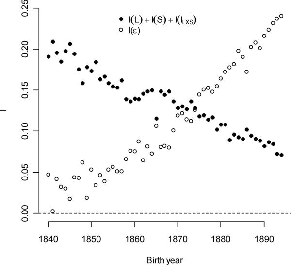
While the opportunity for sexual selection increased slowly over time, two of its sources changed in opposite ways. Contribution from individual polygyny averaged 0.00997 (1.8% of total I), but per-cohort contributions declined from a maximum of 0.0421 in 1840 (7.4% of total I). This decline slowed over time, especially after 1870. Female ever-mating success explained more I with time, increasing by 0.00088/year (an annual increase of 1.20% relative to its initial value). While male ever-mating explained an important part of I in all years (averaging 16.0% of its total), its absolute contribution increased less than female ever-mating (0.388% relative to the initial value). Together, male and female ever-mating explained 30.3% of I. Individual polyandry never explained more than 0.24% of I in any birth year, and its contribution to I averaged over all cohorts was 0.031%. The conditioning traits (sex, survival, and sex-by-survival interactions) explained 24.0% of I averaged over all cohorts, but its absolute contribution declined over time (−0.00225/year – see Figure 8b). The average amount of I that was left unexplained by the fitness model was 19.4% of the averaged total. The absolute contribution of error variance to I increased annually by 3.71% of its initial value.
Figure 8B.
Variation in survival, sex, and their interaction explained progressively less of the opportunity for selection with time. Unexplained fitness variation increased, however.
Discussion
The strength of selection for individual and parental mate number was measured separately in 55 consecutive birth year cohorts to resolve secular trends in the strength of precopulatory sexual selection. Two conceptual innovations set this study apart. First, demographic realism was added to the definition of individual fitness by incorporating age-structure and population growth. Second, the meaning of sexual selection was expanded to include selection acting through parental mating success. The strength of sexual selection in a human population was quantified in two ways. The first is selection for fitness, measured in terms of the opportunity for selection, or the variance in relative fitness. This addresses the question: How much potential does selection for all traits (measured or not) or on particular traits (e.g., mating success) have to improve the fitness of a population? The second measure is selection for specific traits, quantified by selection gradients and the covariances between traits and relative fitness. As I show below, an understanding of how selection gradients, including individual- and family-level Bateman gradients, change can tell us a great deal about why the opportunity for selection changes.
Why did the opportunity for selection change?
The total opportunity for selection was a U-shaped function of birth year, with similar values at the beginning and at the end of the study period. This trajectory closely tracks that reported by Moorad et al (2011), although absolute values are slightly lower here (Figure 7). The slight suppression of I in this study may reflect the definition of fitness that relaxes the often implicit assumption that generations do not overlap (Fisher 1958; Hamilton 1966; Charlesworth 1994). This discounting suppressed the fitness variance caused by late-life reproductive variance.
The opportunities for selection in the female-only population (Moorad 2013) followed a very different trajectory than that reported in this two-sex studies (Figure 7). Females alone did not exhibit the initial decline in I. I interpret the U-shaped pattern described here as arising from two co-occurring and antagonistic processes. First, changes in population growth rates (Figure 1) point to a fertility transition beginning in the late 1850s birth year cohorts. Mean lifetime reproduction declined in females over the same years (Moorad 2013). This female-only study analyzed selection for age-specific fertility, a more direct determinant of fitness than mating success (see Appendix), and it demonstrated that selection gradients for reproduction at all ages increased as a direct consequence of declining population growth rates. These changes caused the strength of female ever-mating selection and its contribution to I to increase over the entire study period (Figs 6A and 8A). Changed female selection could not have caused I to decline in the earliest years of the study, however.
If females did not contribute to the dramatic initial decline in I, then changing selection for male traits must. Indeed, decreased selection gradients for individual-level polygyny and expressed polygyny variance (Figs 3B, 5B) contributed to the decline in I over the first half of the study period (Fig 8A). Both changes likely had the same cause: a mating system transition during which marriage practices changed. Reduced polygamy lessened the rates of polygyny (Fig 2), which decreased the expressed polygyny variance. The association between the mating system transition and the individual male Bateman gradient is less obvious but can be explained. Polygamists produced more children than serial monogamists on a per-mate basis (Moorad et al. 2011). At the beginning of the study period, polygyny was caused by both polygamy and serial monogamy, but as polygamy rates declined, Bateman gradients progressively reflected more the weaker relationship between multiple-mating and fitness in the serial monogamists.
How important was sexual selection?
The ratio of the opportunity for sexual selection (Is) to the opportunity for selection (I) can be thought of as a measure of the relative potential for sexual selection to increase fitness (Wade and Shuster 2004a). Moorad et al (2011) reported that Is:I fell from approximately 40% to 22% over the years 1840 to 1894 (a decline of approximately one-half in absolute terms). In contrast, this study finds that the proportional contribution to total selection explained by directional selection for mating success (ever-mating and multiple-mating) increased slightly over these years from approximately 30 to 35% (from 0.170 to 0.199 in absolute terms). While the contribution of polygyny variance to I fell with the decline in polygamy, the contribution of ever-mating to I increased faster and over the entire study period owing to increased juvenile survival and decreased mating rates among surviving adults. In terms of contributions to Is, individual-level selection for ever-mating was more important than selection for multiple-mating in both sexes (as predicted by Shuster and Wade (2003)).
There are three possible reasons to explain why the two studies find different secular changes in the strength of sexual selection. First, fitness is defined differently in the two studies, but it is not clear how exactly this difference may have contributed to the qualitatively divergent results. A second, and more persuasive, argument may be that differential juvenile mortality contributed to mating success variance in Moorad et al (2011) but not here. If one chooses to define sexual selection in such a way as to control for the effects on pre-reproductive mortality on fitness (e.g., Courtiol et al. 2012), then declines in juvenile mortality, such as experienced by the Utah population, will not directly reduce the strength of sexual selection. In other words, juvenile mortality variance will contribute directly to I but not to Is. Third, Is, as it is usually defined (Wade 1979; Arnold and Wade 1984; Shuster and Wade 2003), includes variation from all traits involved in mate number, observed or not. Here, only those traits that are explicitly included in the linear model of fitness and that contribute to sexual selection are included (ever-mating and multiple-mating, but not pre-reproductive mortality, sex, or their interaction). In addition, non-linear selection for mating success can contribute to Is (Moorad and Wade 2013), but these contributions are not investigated here.
How important is group selection?
Individual polygyny was strong, but it provided less of a benefit to male fitness than suggested by Moorad et al (2011). Quantified in terms of selection gradients, sire polygyny appeared to have been weakly beneficial. However, the strength of selection for sire polygyny matched the strength of individual-level selection over the study period owing to far greater sire polygyny variance. There was a small fitness advantage given to females who mated more than once and an equally small benefit delivered to their children. Family-level selection for polyandry was far weaker than family-level selection for polygyny but stronger than individual-level selection for polyandry. For the purposes of predicting a response to selection, however, the efficacy of a given amount of family-level selection should be less than that of a similar amount of individual-level selection (Falconer 1965; Cheverud 1984; Cheverud and Moore 1994; Wade 1998; Wolf and Brodie 1998; Bijma and Wade 2008; McGlothlin et al. 2010). For parental effects, and assuming a value of relatedness between parents and offspring of one-half, selection for parental phenotypes must be twice as strong as selection for individual phenotypes to produce equitable effects. Weighted in this way, family-level polygyny selection is half the strength of individual-level polygyny selection, and family-level polyandry selection is twice the strength of polyandry selection.
Family-level selection for sire polygyny is consistent with an earlier observation from this population that polygamy is associated with higher offspring fertility (Josephson 1993). However, it would not be safe to assume that increased offspring fitness is the rule among all polygynous human population. For example, Borgerhoff Mulder (1989) found no relationship between sire polygyny and offspring survival in the Kipsigis. These are important issues for the evolution of the human mating system, especially with respect to tests of the “polygyny – threshold” model (Orians 1969; Bean and Mineau 1986; Anderton and Emigh 1989; Marlowe 2000; Moorad et al. 2011), where it is important to quantify the fitness cost to females who choose polygynous males with superior territories over monogynous males with inferior territories. If these fitness costs are too great, females will be selected to forgo mating with polygynous males even if they offer superior environments. The multi-level perspective shows how family-level selection acting on sire polygyny can shift the calculus of female mate-choice: if sire polygyny is advantageous to individuals, then selection in the offspring will act to increase selection for females to choose polygynous mates. If polygyny is directly deleterious to the female, as it may be in this population (Josephson 1993; Moorad et al. 2011), then there will be conflict between levels of selection for female mate choice. In a sense, the multilevel selection perspective formalizes relationships examined in the anthropological literature that link marriage-type (polygamy vs. monogamy) to offspring fitness components. It is superior to the grandchild-scoring approach because it defines explicitly the relationships between fitness and traits in parents and offspring. Differently put, the multilevel perspective correctly delineates the fitness of parents and their offspring (Wolf and Wade 2001).
Conclusion
Parents' mating success positively influenced their childrens' fitness. The strength of sire polygyny selection approximated that for individual polygyny, and the strength of selection for dam polyandry was greater than that for individual polyandry. However, selection for fitness was dominated by variation among individual-level phenotypes. Traits that affect polygyny or polyandry are under stronger selection than would be indicated under a model of fitness that considers only individual characters. These results show that sexual selection is a multi-level process and that future studies should account for contextual traits, such as parental mating success. I applied demographic theory to yield a more general definition of individual fitness that accounts for age-structure and overlapping generations. These conditions apply to many study systems, and they certainly characterize all human populations. The results presented here suggest that demographic realism should be taken into account in future studies of sexual selection.
Supplementary Material
Acknowledgments
The work was funded by NIH T32AG000139. I thank Michael Wade and Susan Alberts for useful discussion and feedback. This paper was much improved by thoughtful comments provided by Charles Goodnight, Daphne Fairbairn, and two anonymous reviewers. I thank the Pedigree and Population Resource (funded by the Huntsman Cancer Foundation) for its role in the ongoing collection, maintenance, and support of the Utah Population Database (UPDB). Requests for data should be addressed to Jahn Barlow at jahn.barlow@hsc.utah.edu. I also acknowledge Dr. Ken R. Smith, Dr. Geraldine P. Mineau and Alison Fraser, MSPH, for their careful management of and assistance with the data used for this study.
Literature Cited
- Andersson MB. Sexual Selection. Princeton University Press; Princeton, N.J.: 1994. [Google Scholar]
- Anderton DL, Emigh RJ. Polygynous fertility - sexual competition versus progeny. Am J Sociol. 1989;94:832–855. doi: 10.1086/229070. [DOI] [PubMed] [Google Scholar]
- Arnold SJ, Duval D. Animal mating systems: A synthesis based on selection theory. The American naturalist. 1994;143:317–348. [Google Scholar]
- Arnold SJ, Wade MJ. On the measurement of natural and sexual selection - theory. Evolution. 1984;38:709–719. doi: 10.1111/j.1558-5646.1984.tb00344.x. [DOI] [PubMed] [Google Scholar]
- Bateman AJ. Intra-sexual selection in Drosophila. Heredity. 1948;2:349–368. doi: 10.1038/hdy.1948.21. [DOI] [PubMed] [Google Scholar]
- Bean LL, Mineau GP. The polygyny-fertility hypothesis: a re-evaluation. Population Studies. 1986;40:67–81. doi: 10.1080/0032472031000141846. [DOI] [PubMed] [Google Scholar]
- Bean LL, Smith KR, Mineau GP, Fraser A. Infant deaths in Utah, 1850–1939. Utah Historical Quarterly. 2002;70:158–173. [Google Scholar]
- Bijma P, Muir WM, Van Arendonk JA. Multilevel selection 1: Quantitative genetics of inheritance and response to selection. Genetics. 2007;175:277–288. doi: 10.1534/genetics.106.062711. [DOI] [PMC free article] [PubMed] [Google Scholar]
- Bijma P, Wade MJ. The joint effects of kin, multilevel selection and indirect genetic effects on response to genetic selection. Journal of Evolutionary Biology. 2008;21:1175–1188. doi: 10.1111/j.1420-9101.2008.01550.x. [DOI] [PubMed] [Google Scholar]
- Borgerhoff Mulder M. Marital status and reproductive performance in Kipsigis women - Re-evaluating the polygyny fertility hypothesis. Pop Stud-J Demog. 1989;43:285–304. [Google Scholar]
- Brown GR, Laland KN, Borgerhoff Mulder M. Bateman's principles and human sex roles. Trends in Ecology & Evolution. 2009;24:297–304. doi: 10.1016/j.tree.2009.02.005. [DOI] [PMC free article] [PubMed] [Google Scholar]
- Canty A, Ripley B. boot: Bootstrap R (S-Plus) Functions. R package version. 2012. [Google Scholar]
- Caswell H. Matrix population models: construction, analysis, and interpretation. Sinauer Associates; Sunderland, Mass: 2001. [Google Scholar]
- Charlesworth B. Evolution in Age-structured Populations. Cambridge University Press; Cambridge, UK: 1994. [Google Scholar]
- Cheverud J, Moore A. Quantitative genetics and the role of the environment provided by relatives in behavioral evolution. In: Boake C, editor. Quantitative Genetic Studies of Behavioral Evolution. University of Chicago Press; Chicago, IL: 1994. pp. 67–100. [Google Scholar]
- Cheverud JM. Evolution by kin selection - a quantitative genetic model illustrated by maternal performance in mice. Evolution. 1984;38:766–777. doi: 10.1111/j.1558-5646.1984.tb00349.x. [DOI] [PubMed] [Google Scholar]
- Clutton-Brock TH, Harvey PH, Rudder B. Sexual dimorphism, socionomic sex ratio and body weight in primates. Nature. 1977;269:797–800. doi: 10.1038/269797a0. [DOI] [PubMed] [Google Scholar]
- Courtiol A, Pettay JE, Jokela M, Rotkirch A, Lumma V. Natural and sexual selection in a monogamous historical human population. Proceedings of the National Academy of Science. 2012;109:8044–8049. doi: 10.1073/pnas.1118174109. [DOI] [PMC free article] [PubMed] [Google Scholar]
- Crow JF. Some possibilities for measuring selection intensities in man. Human Biology. 1958;30:1–13. [PubMed] [Google Scholar]
- Damuth J, Heisler IL. Alternative formulations of multilevel selection. Biol Philos. 1988;3:407–430. [Google Scholar]
- Darwin C. The Descent of Man and Selection in Relation to Sex. J Murray; London: 1871. [Google Scholar]
- Davison AC, Hinkley DV. Bootstrap Methods and Their Applications. Cambridge University Press; Cambridge: 1997. [Google Scholar]
- Falconer DS. Maternal effects and selection response. Genetics today: proceedings of the XI International Congress of Genetics; The Hague, The Netherlands. New York: Macmillan; Sep, 1965. pp. 763–774. 1963. [Google Scholar]
- Fisher RA. The Genetical Theory of Natural Selection. Oxford University Press; Oxford, UK: 1958. [Google Scholar]
- Gillespie DOS, Russell AF, Lumma V. When fecundity does not equal fitness: evidence of an offpsring quantity versus quality trafe-off in pre-industrial humans. Proceedings of the Royal Society B. 2008;275:713–722. doi: 10.1098/rspb.2007.1000. [DOI] [PMC free article] [PubMed] [Google Scholar]
- Goodnight CJ, Schwartz JM, Stevens L. Contextual analysis of models of group selection, soft selection, hard selection, and the evolution of altruism. American Naturalist. 1992;140:743–761. [Google Scholar]
- Hamilton WD. Moulding of senescence by natural selection. Journal of theoretical biology. 1966;12:12–45. doi: 10.1016/0022-5193(66)90184-6. [DOI] [PubMed] [Google Scholar]
- Heisler IL, Damuth J. A method for analyzing selection in hierarchically structured populations. American Naturalist. 1987;130:582–602. [Google Scholar]
- Hersch EI, Phillips PC. Power and potential bias in field studies of natural selection. Evolution. 2004;58:479–485. [PubMed] [Google Scholar]
- Hill K, Lancaster J, Bock A, Johnson SE. Does observed fertility maximize fitness among New Mexican men? A test of an optimality model and a new theory of parental investment in the embodied capital of offspring. Human Nature. 1995;6:325–360. doi: 10.1007/BF02734205. [DOI] [PubMed] [Google Scholar]
- Jones AG. On the opportunity for sexual selection, the Bateman Gradient and the maximum intensity of sexual selection. Evolution. 2009;63:1673–1684. doi: 10.1111/j.1558-5646.2009.00664.x. [DOI] [PubMed] [Google Scholar]
- Jones AG, Avise JC. Mating systems and sexual selection in male-pregnant pipefishes and seahorses: insights from microsatellite-based studies of maternity. Journal of Heredity. 2001;92:150–158. doi: 10.1093/jhered/92.2.150. [DOI] [PubMed] [Google Scholar]
- Josephson SC. Status, reproductive success, and marrying polygynously. Ethology and Sociobiology. 1993;14:391–396. [Google Scholar]
- Krakauer AH, Webster MS, Duval EH, Jones AG, Shuster SM. The opportunity for sexual selection: not mismeasured, just misunderstood. Journal of Evolutionary Biology. 2011;24:2064–2071. doi: 10.1111/j.1420-9101.2011.02317.x. [DOI] [PubMed] [Google Scholar]
- Lande R, Arnold SJ. The measurement of selection on correlated characters. Evolution. 1983;37:1210–1226. doi: 10.1111/j.1558-5646.1983.tb00236.x. [DOI] [PubMed] [Google Scholar]
- Lofredo CA, Borgia G. Sexual selection, mating systems, and the evolution of avian acoustical displays. American Naturalist. 1986;128:773–794. [Google Scholar]
- Mace R. The coevolution of human fertility and wealth inheritance strategies. Philos T R Soc B. 1998;353:389–397. doi: 10.1098/rstb.1998.0217. [DOI] [PMC free article] [PubMed] [Google Scholar]
- Marlowe FW. Paternal investment and the human mating system. Behav Process. 2000;51:45–61. doi: 10.1016/s0376-6357(00)00118-2. [DOI] [PubMed] [Google Scholar]
- McGlothlin JW, Moore AJ, Wolf JB, Brodie ED. Interacting phenotypes and the evolutionary process. III. Social evolution. Evolution. 2010;64:2558–2574. doi: 10.1111/j.1558-5646.2010.01012.x. [DOI] [PubMed] [Google Scholar]
- Moorad JA. A demographic transition altered the strength of selection for fitness and age-specific survival and fertility in a 19th century American population. Evolution. 2013 doi: 10.1111/evo.12023. In press. [DOI] [PMC free article] [PubMed] [Google Scholar]
- Moorad JA, Promislow DEL, Smith KR, Wade MJ. Mating system change reduces the strength of sexual selection in an American frontier population of the 19th century. Evolution and Human Behavior. 2011;32:147–155. doi: 10.1016/j.evolhumbehav.2010.10.004. [DOI] [PMC free article] [PubMed] [Google Scholar]
- Moorad JA, Wade MJ. Selection gradients, the opportunity for selection, and the coefficient of determination. American Naturalist. 2013 doi: 10.1086/669158. In press. [DOI] [PMC free article] [PubMed] [Google Scholar]
- O'Donald P. Change of fitness by selection for a quantitative character. Theoretical population biology. 1970a;1:219–232. doi: 10.1016/0040-5809(70)90036-5. [DOI] [PubMed] [Google Scholar]
- O'Donald P. Measuring the change of population fitness by natural selection. Nature. 1970b;227:307–308. doi: 10.1038/227307a0. [DOI] [PubMed] [Google Scholar]
- Okasha S. Multi-level selection, covariance and contextual analysis. British Jnl. for the Philosophy of Sci. 2004;55:481–504. [Google Scholar]
- Orians GH. On Evolution of Mating Systems in Birds and Mammals. American Naturalist. 1969;103:589–603. [Google Scholar]
- Price GR. Selection and covariance. Nature. 1970;227:520–521. doi: 10.1038/227520a0. [DOI] [PubMed] [Google Scholar]
- R Development Core Team . R: A language and environment for statistical computing. The R Foundation for Statistical Computing; Vienna, Austria: 2011. [Google Scholar]
- Robertson A. A mathematical model of culling process in dairy cattle. Animal Production. 1966;8:95–108. [Google Scholar]
- Shuster SM, Wade MJ. Mating Systems and Mating Strategies. Princeton University Press; Princeton, N.J.: 2003. [Google Scholar]
- Smith JE, Kunz PR. Polygyny and fertility in nineteenth-century America. Population Studies. 1976;30:465–480. [PubMed] [Google Scholar]
- Wade MJ. Sexual selection and variance in reproductive success. American Naturalist. 1979;114:742–747. doi: 10.1086/424531. [DOI] [PubMed] [Google Scholar]
- Wade MJ. The ecology of sexual selection - mean crowding of females and resource-defense polygyny. Evolutionary Ecology. 1995;9:118–124. [Google Scholar]
- Wade MJ. The evolutionary genetics of maternal effects. In: Mousseau T. A. a. C. W. F., editor. Maternal Effects as Adaptations. Oxford University Press; Oxford, U.K.: 1998. pp. 5–21. [Google Scholar]
- Wade MJ, Arnold SJ. The intensity of sexual selection in relation to male sexual behavior, female choice, and sperm precedence. Animal Behaviour. 1980;28:446–461. [Google Scholar]
- Wade MJ, Shuster SM. Estimating the strength of sexual selection from Y-chromosome and mitochondrial DNA diversity. Evolution. 2004a;58:1613–1616. doi: 10.1111/j.0014-3820.2004.tb01741.x. [DOI] [PubMed] [Google Scholar]
- Wade MJ, Shuster SM. Sexual selection: Harem size and the variance in male reproductive success. American Naturalist. 2004b;164:E83–E89. doi: 10.1086/424531. [DOI] [PubMed] [Google Scholar]
- Walsh JB, Lynch M. Individual Fitness and the Measurement of Univariate Selection. Evolution and Selection of Quantitative Traits. 2008 [Google Scholar]
- Wolf JB, Brodie ED. The coadaptation of parental and offspring characters. Evolution. 1998;52:299–308. doi: 10.1111/j.1558-5646.1998.tb01632.x. [DOI] [PubMed] [Google Scholar]
- Wolf JB, Wade MJ. On the assignment of fitness to parents and offspring: whose fitness is it and when does it matter? Journal of Evolutionary Biology. 2001;14:347–356. [Google Scholar]
Associated Data
This section collects any data citations, data availability statements, or supplementary materials included in this article.


