

Abstract
We developed an EXpectation Propagation LOgistic REgRession (EXPLORER) model for distributed privacy-preserving online learning. The proposed framework provides a high level guarantee for protecting sensitive information, since the information exchanged between the server and the client is the encrypted posterior distribution of coefficients. Through experimental results, EXPLORER shows the same performance (e.g., discrimination, calibration, feature selection etc.) as the traditional frequentist Logistic Regression model, but provides more flexibility in model updating. That is, EXPLORER can be updated one point at a time rather than having to retrain the entire data set when new observations are recorded. The proposed EXPLORER supports asynchronized communication, which relieves the participants from coordinating with one another, and prevents service breakdown from the absence of participants or interrupted communications.
Keywords: Clinical information systems, Decision support systems, Distributed privacy-preserving modeling, Logistic regression, Expectation propagation
1. INTRODUCTION
Frequentist logistic regression [1] has a long and successful history of useful applications in biomedicine, including various decision support applications, e.g., anomaly detection [2] survival analysis [3], and early diagnosis of myocardial infarction [4]. Despite its simplicity and interpretability, the frequentist logistic regression approach has limitations. It requires training data to be combined in a centralized repository and cannot directly handle distributed data (the scenario in many biomedical applications [5]). It has been shown in last decade that data privacy cannot be maintained by simply removing patient identities. For example, Sweeney showed that a simple combination of [date of birth, sex, and 5-digit zip code] was sufficient to uniquely identify over 87% of US citizens [6]. Due to privacy concerns, training data in one institute cannot be exchanged or shared with other institutes directly for the purposes of global model learning. To address such a challenge, many privacy-preserving models have been studied [7, 8, 9, 10]. Among the most popular ones, privacy-preserving methods based on secure multiparty computing (SMC) [11, 12, 13, 14, 15] (i.e., building accurate predictive models without sharing raw data) do not change the results and seem practical compared to solutions based on data generalization and perturbation [16, 17, 18, 19] that change results.
For distributed model learning with multiple sites, a common scenario is that each site has a subset of records with the same fields, which is usually referred to as horizontally partitioned data. In this paper, we focus on the horizontally partitioned data for distributed logistic regression learning in Bayesian paradigm. During the past decade, numerous privacy-preserving/secure distributed frequentist regression models for horizontally partitioned data [20, 21, 22, 23, 24, 25, 26] have been studied. For example, the DataSHIELD framework [20] provides a secure multi-site regression solution without sacrificing the model learning accuracy. However, in the above multi-site regression frameworks, the information matrix and score vector exchanged among multiple sites may result in information leakage during each learning iteration [27, 28]. To mitigate privacy and security risks, Karr and Fienberg et. al. studied numerous SMC based distributed regression model [21, 22, 23, 24, 25]. Unfortunately, as mentioned by El Emam et.al in [26], aforementioned approaches can still potentially leak sensitive personal information. Therefore, the authors [26] proposed a secure distributed logistic regression protocol to offer stronger privacy/security protection. The computational complexity of the above protocol grows exponentially with the increase of site number.
The closest work for the method presented here is the Grid LOgistic REgression (GLORE) model [29] and the Secure Pooled Analysis acRoss K-site (SPARK) protocol [26], which train frequentist logistic regression model in a distributed, privacy-preserving manner. GLORE leverages non-sensitive decomposable intermediary results (i.e., calculated at an individual participating site) to build an accurate global model. However, as GLORE does not use any SMC protocol, there is no provable privacy guarantee. SPARK protocol uses secure building block (e.g., secure matrix operation, etc.) to develop a secure distributed logistic regression protocol. However, SPARK will not scale well for a large distributed network, as its complexity grows exponentially with the network size. Both GLORE and SPARK require synchronized communication among participants (i.e., all parties had to be simultaneously online for multiple iterations of training until convergence). Additionally, the frequentist logistic regression approach is inefficient in learning data that are frequently being updated, because the model needs to be completely retrained when they receive any additional observations.
We propose a Bayesian alternative for the distributed frequentist logistic regression model, which we call EXpectation Propagation LOgistic REgRession (EXPLORER). EXPLORER offers distributed privacy-preserving online model learning. The Bayesian logistic regression model was described previously by Ambrose et al. [30], who compared it with the frequentist logistic regression model in terms of performance. Marjerison also discussed Bayesian logistic regression [31] and suggested a Gibbs sampling based optimization, which unfortunately is very time-consuming operation. However, both papers assumed a centralized computation environment, and privacy was not taken into consideration. In comparison, EXPLORER focuses on privacy preservation and it is based on an efficient state-of-the-art inference technique (i.e., expectation propagation [32]). To the best of our knowledge, EXPLORER is the first paper addressing distributed logistic regression in the Bayesian setting. EXPLORER handles some shortcomings of the frequentist logistic regression approach and other frequentist SMC models, as illustrated in Table 1.
Table 1.
Comparing EXPLORER with GLORE (as well as other frequentist SMC models)
| Privacy-preserving | Asynchronous communication | Online learning | |
|---|---|---|---|
| GLORE (and other frequentist SMC models) | x | ||
| EXPLORER | x | x | x |
The major contributions of this paper are as follows: we propose a Bayesian approach for logistic regression that takes the privacy issue into account. Just like GLORE and SPARK, the EXPLORER model learns from distributed sources, and it does not require access to raw patient data. In addition, it provides online learning capability to avoid the need for training on the entire database when a single record is updated. Furthermore, EXPLORER supports asynchronous communication so that participants do not have to coordinate one another. This prevents service breakdowns that result from absence of participants or communication interruptions. Finally, we introduced Secured Intermediate iNformation Exchange (SINE) protocol to enhance the security of the proposed EXPLORER framework, in order to further reduce the risk of information leak during the exchange of unprotected aggregated statistics. The proposed SINE protocol offers provable security and light-weighted computation overhead to ensure the scalability of the EXPLORER framework.
2. Methodology
We start with a quick review of the logistic regression (LR) model. Assume a training dataset D = {(x1, y1), (x2, y2), · · ·, (xm, ym)}, where yi ∈ {0, 1} and xi are the binary label and the feature vector of each record, respectively, with i = 1, · · ·, m. We denote by Y = {y1, · · ·, ym} the set of binary labels. The posterior probability of a binary event (i.e., class label) yi = 1 given observation of a feature vector xi can be expressed as a logistic function acting on a linear function βT xi so that
| (1) |
where the parameter vector β corresponds to the set of coefficients that need to be estimated and that will be multiplied by the feature vector xi (i.e., βTxi) to make predictions. In this paper, we drop the feature vector xi from the likelihood function and denote P (yi = 1 | xi, β) as P (yi= 1 | β) to allow a more compact notation.
To estimate β from training datasets, existing learning algorithms can be categorized into two classes, Maximum Likelihood (ML) estimation and Maximum a Posterior (MAP) estimation. The procedures of estimating model coefficients through ML and MAP estimators are elaborated in the supplementary materials - Sections S3 and S4. In this paper, we focus on the MAP estimation for the proposed EXPLORER framework.
3. Framework of EXPLORER
In this section, we introduce the EXPLORER framework based on a factor graph, which enables the independent inter-site update of all the participating sites without performance loss. In a nutshell, a factor graph is a bipartite graph (see supplementary materials - Sections S1 and S2) that comprises two different kinds of nodes (i.e., a factor node (square) and a variable node (circle)). In a factor graph, each edge must connect a factor node and a variable node. The joint probability over all variables can be expressed as products of some factor functions in which each contains only a subset of all variables as arguments and is represented by a factor node. Each variable node expresses a random variable. EXPLORER requires two phases: initially the updates on coefficients must be made on each site (i.e., intra-site update), and then updated across sites (i.e., inter-site update).
3.1. Intra-site update
Although we are interested in the distributed online model learning, let us first explain how each participating site updates its own posterior distribution (i.e., intra-site update). In general, the posterior probability of the j-th site with j = 1, 2, · · ·, n can be expressed as
| (2) |
where we introduce mh<sub>j</sub>→B<sub>j</sub>(βj) and to capture the prior probability and the likelihood function, respectively. Moreover, mj is the total number of records in the first j sites with m0 = 0. However, the direct evaluation of the above posterior is mathematically intractable, thus we need to resort to the Expectation propagation (EP) algorithm, a deterministic approximate inference method. In the proposed EXPLORER framework, we introduce an approximate function representing a normal distribution for each true likelihood function . Therefore, the approximate posterior distribution can be expressed as
| (3) |
Based on the above factorization, we first introduce a variable node Bj (i.e., site header) to capture the approximate posterior distribution q(βj). We introduce extra factor nodes hj and to capture the prior probability and the likelihood function (see Fig. 1), respectively. The update of the approximate likelihood function relies on the factor graph based-EP algorithm (see Appendix A. for details).
Figure 1.
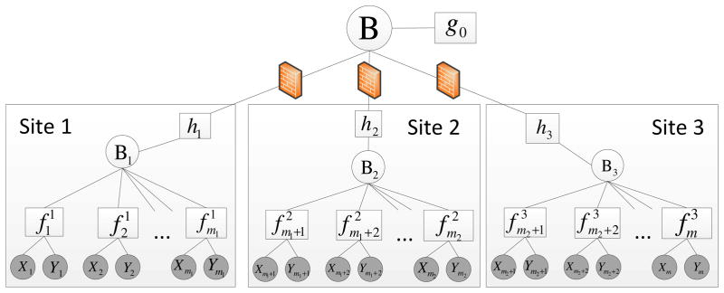
Factor graph of EXPLORER with 3-site asynchronous update.
The details of intra-site update rules in EXPLORER are listed in Algorithm 1 (A1). Since we are using the Normal distribution as our approximate distribution, messages exchanged between the factor nodes and the variable nodes can be parameterized by the mean vector and its covariance matrix. The intra-site update starts from the initialization step (A1: line 1), where all the messages are initialized as uniform distributions with zero mean and infinite variance for a new model learning task. However, for an online learning task with previous results, we need to initialize the messages using their previous status. The approximate posterior is initialized as the product of prior and all the approximate likelihood functions. We can iteratively update the approximate posterior distribution of each site until it converges through A1 from lines 2 to 7. The key idea of EP is to sequentially update the approximate posterior distribution qi (βj) by incorporating a single true likelihood function as shown in line 5. For more details about EP-based LR, please refer to Appendix A.
Algorithm 1.
Intra-site Posterior update in EXPLORER
| 1: | Initialize : each approximate likelihood function and approximate posterior n |
| 2: | Repeat |
| 3: | for all records i = mj−1 + 1, · · ·, mj do |
| 4: | Get partial posterior function q\i (βj) by removing the approximate factor from the approximate posterior: |
| 5: | Update q(βj) by incorporating a single true likelihood function according to Assumed Density Filtering (ADF) [33]: |
| 6: | Set the approximate factor: |
| 7: | end for
|
| 8: | Until parameters converge |
3.2. Inter-site update
To achieve asynchronous inter-site update (see Fig. 1), we introduce an additional variable node B (i.e., server node) to capture the global posterior probability learnt from all sites. Then, we connect each factor node hj with the server variable node B for exchanging messages among sites. We assume that all sites share the same prior information, which is captured by the factor node g0. The inter-site update of each approximate posterior qj (βj) relies on a powerful message passing algorithm (i.e., belief propagation (BP)), which has been widely used in Bayesian inference on factor graphs (see Appendix B for details). Based on this framework, we can update sites in an asynchronous way.
Algorithm 2.
Inter-site posterior update in asynchronous EXPLORER
| 1: |
Global initialization: Initialize all the messages mB→h<sub>j</sub>(β) and mh<sub>j</sub>→B (β) between server variable node B and clients factor nodes hj, where the subscriptions B → hj and hj → B indicate the message directions. |
|
|
|
||
| 2: | Local initialization for all the online sites: | |
|
|
||
| 3: | Initialize messages mB<sub>j</sub>→h<sub>j</sub> (β) and each approximate likelihood function with i = mj−1 + 1, · · ·, mj. | |
|
|
||
| 4: | Repeat: | |
|
|
||
| 5: | for all the online sites (parallel update) | |
|
|
||
| 6: | Update intra-site message: mh<sub>j</sub>→ B<sub>j</sub>(βj)= ∫ δ(β, βj) mB→h<sub>j</sub> (β) dβ | |
|
|
||
| 7: | Set approximate posterior: | |
|
|
||
| 8: | Update approximate posterior qj(βj) according to Algorithm 1. | |
|
|
||
| 9: | Update intra-site messages at variable node Bj :
|
|
|
|
||
| 10: | Upload message at factor node hj :
|
|
|
|
||
| 11: | end for | |
|
|
||
| 12: | Send out message at server node B:
|
|
|
|
||
| 13: | Until parameters converge | |
|
|
||
| 14: | Get the final approximate posterior distribution by multiply- ing all the incoming messages at the server node B. |
The details of the proposed asynchronous EXPLORER are listed in Algorithm 2 (A2). The asynchronous inter-site update starts from the global and local initialization steps (A2: line 1 to 2), which follow the same initialization rules as those for the intra-site update. Then, we can iteratively update the approximate posterior distribution of each site until it converges via A2 from lines 4 to 12. In A2 line 6, we choose delta function δ(βj, β) as a factor function of the factor node hj, which follows the suggestion in [34] for mathematical convenience (see Appendix B. for details). Lines 6 and 7 show the factor node and variable node updates according to the BP algorithm. In line 8, we perform an intra-site update according to Algorithm 1. Then, in line 9, we update the message from variable node Bj to factor node hj. Finally, factor node hj commits its message to the server node according to line 10, where the message can be interpreted as the belief that the server node should take value β from the j-th site. When the server node has collected all the updates from the corresponding online sites, it can send the aggregated information back to each site as in line 12. Finally, the approximate posterior can be obtained by multiplying all the incoming messages at the server node B as in line 14. The asynchronous EXPLORER allows client sites to dynamically shift from online to offine modes as needed. The impacts of sites with different data size on convergence speed have been studied in the results section. The proposed EXPLORER framework is based on the EP algorithm, which is guaranteed to converge to a fixed point for any given dataset [32].
3.3. Distributed feature selection
Feature selection is important to logistic regression analysis. In this sub-section, we introduce the distributed forward feature selection (DFFS) protocol, which is based on the traditional forward feature selection (FFS) algorithm [35], but tailored for the EXPLORER framework. To better understand DFFS protocol, let us start with a quick review of traditional FFS algorithm.
Suppose there are d candidate features (i.e., xall = {x1, x2, · · ·, xd}). In the first iteration, the FFS algorithm starts by taking only one feature into account at each time, so that one can find the best individual feature for s1 = 1, 2, · · ·, d, which could result in the best classification performance. Then, in the second iteration, FFS algorithm tries to find the best subset in terms of classification performance, where xs<sub>2</sub> is chosen from the remaining d − 1 features in xall. We repeat the aforementioned procedures, until the currently best subset at iteration k + 1 degrades the classification performance obtained through the subset . Finally, the is treated as the output of FFS algorithm. In traditional centralized regression model, the classification performance is usually measured through averaged classification accuracy using cross validation. However, in a distributed environment, it is usually infeasible to perform cross validation over distributed sites, which motivated us to develop the following DFFS protocol.
In our proposed DFFS, suppose there are n participant sites. Then, we create n EXPLORER instances at the server side with n − 1 participant sites in each instance in parallel, where the j-th site is excluded from the j-th EXPLORE instance, but it serves as the testing data for the j-th EXPLORE instance. For example, given a candidate feature subset with l features, the j-th EXPLORER instance can first learn a logistic regression model based on all the participant sites except the j-th site. The j-th EXPLORER instance can send its learnt model to the j-th site to verify its classification performance. Then, the j-th site can report the classification accuracy back to the server. It is worth mentioning that the information exchanged between the j-th site and the server node are aggregated information. Since there are n parallel EXPLORER instances at the server side, the server can calculate an averaged classification accuracy based on the reports from each instance, which is analogous to a centralized n cross validation. The averaged classification accuracy can be used as the criteria for selecting the best at the l DFFS iteration. Then, all the EXPLORER instances will move to the (l + 1)-th DFFS iteration. By repeating the above procedures, we can find the best feature subset with the maximum classification performance.
3.4. Secured intermediate information exchange
The information exchanged among all participant sites in EXPLORER framework are the posterior distribution of the model parameter β, which is assumed as normal distribution and captured by the mean vector and the covariance matrix. Compared with raw data, the posterior distribution (i.e., the mean vector and the covariance matrix) only reflects the aggregated information of the raw data rather than information based on individual patients, which has already reduced the privacy risk. However, as identified by previous studies [27, 28, 26], aggregated information may potentially leak private information. We propose a Secured Intermediate iNformation Exchange (SINE) protocol as an optional module for further enhancing the confidentiality of the EXPLORER framework.
As we illustrated in the Section 3.2, the posterior distribution of the global model parameter is calculated by multiplying all the incoming messages from n sites at the server node. In the context of Gaussian distribution, the global distribution obtained through the multiplication of all the incoming messages [36] can be captured by its mean vector μ and covariance matrix V as follows,
| (4) |
| (5) |
where Vj and μj are the covariance matrix and the mean vector obtained from the j-th site (j = 1, 2, · · ·, n), respectively. The proposed SINE protocol is mainly based on the modified secure sum algorithm, which offers provable security guarantee [37, 24].
The SINE protocol, as shown in Fig. 2, begins by generating a pair of secure random matrices (with size d × d) and (with size d × 1) at each participant site before the start of each learning iteration, where d is the dimension of μj. Meanwhile, the server also generates a pair of random matrix and random vector with the same size as these of and . Then, the server sends and to a randomly selected site (e.g., the j-th site). The j-th site adds its own and with the received and and sends the summation to its neighboring site according to the standard secure sum protocol. Finally, the last site send its summation (i.e., and ) back to the server node. According to the secure sum protocol, the server can easily recover the summation and , as and were generated at the server side.
Figure 2.

Secured intermediate information exchange (SINE) protocol.
Now, for secure information exchange among client sites and server, each client site can send out the secured information and instead of the raw information and , respectively. Then, at the server side, one can easily recover the true summation and , where the aggregations of and are obtained in the current step and the summations of and are already obtained in the previous step. It is worth mentioning that unlike frequentist LR where the information matrix must be passed through all participant sites, in EXPLORER, each Vj and μj can be updated independently by each site and aggregated at the server node, which reduces the privacy and collusion risks by avoiding the inter-site communication of sensitive information. The following is the proof of security of the proposed SINE protocol based on secure summation principle [38].
Proof of security of the SINE protocol
Let’s suppose rk,l and vk,l are two elements at the k-th row and the l-th column of the secure random matrix and the covariance matrix , respectively. We also suppose that vk,l is known to lie in the range [−10M, 10M), which can be validated by selecting a significantly large number for M (e.g., M = 50). Then, rk,l is a randomly selected floating number with maximum precision at 10−N-th digits from the range [−10M, 10M), which means there are total 2 × 10N+M possible choices for any rk,l. Given the summation at the attacker side, the probability to gain the original information (i.e., v̂k,l = vk,l) can be expressed as,
where v̂k,l and r̂k,l are the estimates of vk,l and rk,l at the attacker side, respectively. Moreover, since there are total d2 elements in , the probability to recover the original covariance matrix can be calculated as , where is the estimate of at the attacker side. Then, we can always select some large numbers for both N and M (e.g., M +N = 100), such that the probability that an attacker can gain the original information is sufficiently small.
4. Experimental results
We evaluated EXPLORER in 5 perspectives with 6 simulated datasets and 5 clinical datasets. Specifically, the perspectives we evaluated include: 1). distributed feature selection, 2). modeling interaction, 3). classification performance, 4). model coefficients estimation, and 5). model convergence. A summary of these 6 simulated and 5 clinical datasets [1, 4, 39] can be found in Table 2, which includes the information of dataset description, number of covariates, number of samples and class distribution for each dataset. The rule of simulated dataset generation will be introduced within each experimental task, where we considered three different types of simulated datasets i.e., independent and identically distributed (i.i.d.) dataset [40], correlated dataset [41] and binary dataset [42]. Moreover, Table 3 shows the detailed descriptions of covariates in each clinical dataset used in our experiment, where numerical covariates are indicated with “*” and categorical variables are converted into binary covariates through dummy coding [43]. For example, a categorical variable with c possible values (e.g., 0, 1 and 2 for c = 3), in dummy coding, will be converted into c−1 binary covariates (e.g., 0 → (0, 0), 1 → (1, 0) and 2 → (0, 1) ).
Table 2.
Summary of datasets used in our experiments, where the class distribution (i.e., the percentage of positive and negative outcome variables) has been listed as reference.
| Dataset | Dataset description | # of covariates | # of samples | Class distribution (positive/negative) |
|---|---|---|---|---|
| 1 | Simulated i.i.d. data | 5 | 500 | 0.618 / 0.382 |
| 2 | Simulated correlated data | 6 | 500 | 0.764 / 0.236 |
| 3 | Simulated i.i.d. data | 15 | 1500 | 0.641 / 0.359 |
| 4 | Simulated correlated data | 15 | 1500 | 0.651 / 0.349 |
| 5 | Simulated binary data | 5 | 500 | 0.846 / 0.154 |
| 6 | Simulated binary data | 15 | 1500 | 0.726 / 0.274 |
| 7 | Biomarker (CA-19 and CA-125) | 2 | 141 | 0.638 / 0.362 |
| 8 | Low birth weight study | 8 | 488 | 0.309 / 0.691 |
| 9 | UMASS aids research | 8 | 575 | 0.256 / 0.744 |
| 10 | Mammography experience study | 8 | 412 | 0.432 / 0.568 |
| 11 | Myocardial infarction | 9 | 1253 | 0.219 / 0.781 |
Table 3.
Feature description for each clinical dataset, where numerical covariates are indicated with “*” and categorical covariates are converted into binary covariates through dummy coding.
| Dataset 7 | Dataset 8 | Dataset 9 | Dataset 10 | Dataset 11 | |
|---|---|---|---|---|---|
| x1 | CA19* | Birth number* | Age* | Symptoms
|
Pain in right arm |
| x2 | CA125* | Smoking status | Beck Depression Score* | Nausea | |
| x3 | - | Race
|
Drug use history
|
Hypo perfusion | |
| x4 | - | Perceived benefit* | ST elevation | ||
| x5 | - | Age of mother* | Prior drug treatments* | Family history | New Q waves |
| x6 | - | Weight at last menstrual period* | Race | Self examination | ST depression |
| x7 | - | - | Treatment assignment | Detection probability
|
T wave inversion |
| x8 | - | - | Treatment site | Sweating | |
| x9 | - | - | - | - | Pain in left arm |
| y | Presence of cancer | Low birth weight | Remained drug free | Mammograph experience | Presence of disease |
4.1. Dataset preparation
In our experiment, each training dataset was created by randomly choosing 80% records from a given dataset and the corresponding testing dataset was generated through the remaining 20% records. Moreover, in order to obtain more reliable results and to be able to compare the results in a statistical way, we conducted each experimental task over 30 trials through the aforementioned method of training/testing datasets generation. Unless explicitly stated, each training dataset was evenly partitioned [29, 26] among all the participant EXPLORER sites. For example, if there are m records in a given training dataset and n participant sites in a task, the sub-dataset possessed by each site is equal to , where we assume that m is divisible by n. In addition, for all 2-site EXPLORER setups of datasets 3 to 11, the difference between means (DBM) of class distribution and covariates of the 2 sites has been shown in Figs. D.6 to D.14 in Appendix D, which offers an intuitive sense about how heterogeneous these sites are.
4.2. Distributed feature selection
Feature selection is an important part of logistic regression analysis. In this sub-section, we studied the distributed feature selection capability of a 5-site EXPLORER setup based on a simulated dataset with 5 covariates, 500 number of records (i.e., the dataset 1 in Table 2). The simulated dataset 1 was generated by drawing samples from 5 independent normally distributed variables [44] with zero means and unit variances, where similar dataset generation strategy has been repeatedly employed in many previous studies [29, 26, 40]. Then, we randomly drew 4 values for the model parameter β from a normal distribution with mean 0 and variance 5 as β = [1.7813, −2.2428, 0, 3.1668, 0, −1.8701]T, where β0 = 1.7813 is the intercept, β2 and β4 are assigned by zeros for the purpose of studying feature selection. Finally, the outcome variable (i.e., classification label) was drawn from a normal distribution with probability of success equal to π(βxi), where π(·) is a logistic function as show in (1) and xi is a vector composed of a constant “1” followed by the aforementioned 5 covariates. As we are interested in the study of feature selection in this task, we treat all 500 records in the simulated dataset 1 as training data and randomly split them into 5 sub-datasets with equal sizes for all participant EXPLORER sites (i.e., 100 records per site) in each experimental trial.
Table 4 shows the feature selection results for simulated dataset 1 using Ordinary LR with FFS algorithm and EXPLORER with DFFS protocol as described in Section 3.3, where β′ and β″ are model parameters averaged over 30 trials learnt by Ordinary LR and EXPLORER, respectively, the Prob. indicates the chance of a given covariate to be selected by either FFS or DFFS algorithms during the 30 trials, and two-sample Z-tests are performed between β′ and β″. In two-sample Z-test, the null and the alternative hypotheses are “β′ = β″” and “β′ ≠ β″”, receptively. In Table 4, we can see both FFS algorithm and the proposed DFFS protocol achieved similar feature selection performance in terms of both qualitative and statistical comparisons, where the model parameters (i.e., β1 to β5) used for generating outcome variable are also listed as a reference. The two-sample Z-test results show that there is no statistically significant difference between β′ and β″. Moreover, for both FFS and DFFS algorithms, the covariates with non-zero model parameters (i.e., βi ≠ 0 for i = 1, 2, · · ·, 5) are fully selected over all 30 trials (i.e., Prob. equals to 1). However, for these covariates with zero model parameters (i.e., βi = 0 for i = 1, 2, · · ·, 5), the chances of selection are quite small (e.g., Prob. is less than 0.3). As we have demonstrated the DFFS capability of the proposed EXPLORER framework, in the rest of our experiments, we assume that all covariates in remaining datasets have been pre-selected.
Table 4.
Feature selection for simulated dataset 1 using Ordinary LR with FFS algorithm and 5-site EXPLORER with DFFS protocol, where β′ and β″ are model parameters averaged over 30 trials learnt by Ordinary LR and EXPLORER, respectively, the Prob. indicates the chance of a given covariate to be selected by either FFS or DFFS during the 30 trials, and two-sample Z-tests are performed between β′ and β″, which show no differences at all.
| True value | Ordinary LR | EXPLORER | two-sample Z-test | ||||
|---|---|---|---|---|---|---|---|
| β′ | Prob. | β″ | Prob. | Test statistic | p-value | ||
| β1 | −2.2428 | −2.0743 | 1.000 | −2.0722 | 1.000 | −0.3573 | 0.7209 |
| β2 | 0.0000 | 0.0452 | 0.267 | 0.0527 | 0.300 | −0.3669 | 0.7137 |
| β3 | 3.1668 | 3.0195 | 1.000 | 3.0167 | 1.000 | 0.5919 | 0.5539 |
| β4 | 0.0000 | −0.0402 | 0.200 | −0.0265 | 0.133 | −0.7003 | 0.4837 |
| β5 | −1.8701 | −1.7313 | 1.000 | −1.7316 | 1.000 | 0.1305 | 0.8962 |
4.3. Model with interaction
Interaction effects in regression reflects the combined impact of variables, which is very important for understanding the relationships among the variables. In this section, we studied a 4-site EXPLORER setup with interaction based on a simulated dataset (i.e., the dataset 2 in Table 2). The simulated dataset 2 was generated by first drawing 500 samples from 3-dimension multivariate normal distribution (i.e., x1, x2, x3) with zero means and randomly generated covariance matrix. Second, we consider the interaction between x1 and x2, x1 and x3, and x2 and x3. Finally, a record vector xi can be represented as xi = [1, x1, x2, x3, x1x2, x1x3, x2x3]T. Moreover, we randomly drew 7 values for the model parameter β = [−1.2078, 2.9080, 0.8252, 1.3790–1.0582, −0.4686, −0.2725]T, where β0 = −1.2078 is the intercept. Then, the outcome variable was drawn from a normal distribution with probability of success equal to π(βxi).
In Table 5, we performed side-by-side comparisons of Hosmer-Lemeshow (H-L) Goodness-of-fit test [45] (i.e., H-L test), and AUCs between model learning with and without interaction for both ordinary LR and EXPLORER. In an H-L test, the null and alternative hypotheses are “the model fits the data well” and “the model does not provide an adequate fit”, respectively. In a two-sample Z-test of AUCs, the null and alternative hypotheses are “AUCs of ordinary LR and EXPLORER are equal” and “AUCs of both models are unequal”, respectively. In Table 5, we can see that both EXPLORER and ordinary LR achieve good H-L test performances. For AUCs, the two-sample Z-test results show that there is no statistically significant difference between AUCs of ordinary LR and EXPLORER. As the simulated dataset 2 was generated with interaction, the AUCs of model with interaction outperform that of model without interaction, which demonstrated that interaction would be an important factor in some regression studies.
Table 5.
H-L tests, qualitative and statistical comparisons of AUCs for simulated dataset 2 with/without interaction using Ordinary LR and 4-site EXPLORER
| With interaction | Without interaction | ||||
|---|---|---|---|---|---|
| Ordinary LR | EXPLORER | Ordinary LR | EXPLORER | ||
| H-L test | test statistics | 22.459 | 40.595 | 15.184 | 18.909 |
| p-value | 0.289 | 0.198 | 0.203 | 0.150 | |
| AUC | Averaged value | 0.851 | 0.852 | 0.794 | 0.793 |
| Standard deviation | 0.045 | 0.045 | 0.058 | 0.058 | |
| Z-test statistics | −0.049 | 0.075 | |||
| Z-test p-value | 0.961 | 0.940 | |||
4.4. Classification performance
Since EXPLORER is proposed for distributed privacy-preserving classification, we are very interested in its classification accuracy and how well the model fits the datasets compared with ordinary LR. In this section, the classification performances are verified over 4 simulated datasets and 4 clinical datasets for total 8 datasets. A brief summary of all aforementioned 8 datasets can be found in Table 2, and the detailed descriptions of covariates of each clinical dataset have been listed in Table 3. Besides the simulated i.i.d. and correlated datasets used in previous tasks, we also included several simulated binary datasets using binomial distribution in this task. Moreover, we carefully chose these simulated and clinical datasets to provide a wider range of class distribution, sample size and number of covariates. All the model parameters β’s for generating outcome variables are randomly sampled from the normal distributions. In this experimental task, we only considered the 2-site EXPLORER setup, where the impact of using different number of participant EXPLORER sites on the model convergence will be discussed shortly in Section 4.6.
First, the H-L test [45] was used to verify the model fit for the proposed EXPLORER. In our experiment, we perform an H-L test at a 5% significance level. Table 6 shows the H-L tests results (i.e., test statistic and p-value) for both EXPLORER and ordinary LR based on aforementioned 8 datasets. There are no conspicuous differences on p-value and test statistic between EXPLORER and ordinary LR for all 8 datasets.
Table 6.
Comparisons of H-L tests for datasets 3 to 10 using Ordinary LR and 2-site EXPLORER
| Dataset ID | Ordinary LR | EXPLORER | ||
|---|---|---|---|---|
| Test statistic | p-value | Test statistic | p-value | |
| 3 | 5.789 | 0.679 | 6.557 | 0.634 |
| 4 | 9.405 | 0.470 | 12.684 | 0.366 |
| 5 | 13.587 | 0.247 | 16.952 | 0.204 |
| 6 | 9.247 | 0.424 | 10.417 | 0.368 |
| 7 | 7.087 | 0.665 | 14.030 | 0.639 |
| 8 | 11.927 | 0.287 | 13.099 | 0.217 |
| 9 | 11.598 | 0.280 | 12.965 | 0.266 |
| 10 | 13.055 | 0.234 | 14.082 | 0.229 |
Second, Table 7 illustrates both the qualitative and statistical comparison of AUCs between Ordinary LR and 2-site EXPLORER based on 8 datasets, where the standard deviation of AUCs are obtained over 30 trials. For qualitative comparison, we can see the maximum difference of AUCs between ordinary LR and EXPLORER is only 0.007. Similarly, in two-sample Z-test of AUCs between ordinary LR and EXPLORER, no statistically significant differences have been observed.
Table 7.
Comparisons of AUCs for datasets 3 to 10 using Ordinary LR and 2-site EXPLORER, where the Std. is the standard deviation of AUCs over 30 trials.
| Dataset ID | Ordinary LR | EXPLORER | two-sample Z test | |||
|---|---|---|---|---|---|---|
| AUC | Std. | AUC | Std. | Test statistic | p-value | |
| 3 | 0.968 | 0.008 | 0.968 | 0.008 | 0.012 | 0.991 |
| 4 | 0.975 | 0.006 | 0.975 | 0.006 | −0.120 | 0.904 |
| 5 | 0.805 | 0.043 | 0.806 | 0.043 | −0.069 | 0.945 |
| 6 | 0.907 | 0.014 | 0.907 | 0.014 | −0.009 | 0.993 |
| 7 | 0.892 | 0.066 | 0.891 | 0.066 | 0.061 | 0.951 |
| 8 | 0.960 | 0.012 | 0.959 | 0.012 | 0.184 | 0.854 |
| 9 | 0.815 | 0.044 | 0.808 | 0.046 | 0.584 | 0.559 |
| 10 | 0.643 | 0.057 | 0.643 | 0.057 | −0.016 | 0.987 |
4.5. Model coefficients estimation
From results above, we demonstrated that the proposed EXPLORER can achieve similar classification and model fit performance when compared with the ordinary LR model. However, in biomedical research, another important aspect of LR is the interpretability of the estimated coefficients β, where the linear function βT xi can be interoperated as the log odds ratios of a binary event yi = 1. Thus, it is also very important to verify that estimated coefficients using the proposed EXPLORER are compatible with those of ordinary LR.
Tables 8 to 11 compare the estimated model coefficients β, their standard deviation over 30 trials, two-sample Z-test of these estimated coefficients between the ordinary LR and 2-site EXPLORER on simulated datasets 3 to 6. The same results for clinical datasets 7 to 10 can be found in Appendix C through Tables C.13 to C.16. The results shown in Tables 8 to 11 and Tables C.13 to C.16 further confirm that EXPLORER and ordinary LR are compatible.
Table 8.
Learnt model parameter β of dataset 3 (Simulated i.i.d. data with 15 covariates) using Ordinary LR and 2-site EXPLORER
| β | Ordinary LR | EXPLORER | two-sample Z test | |||
|---|---|---|---|---|---|---|
| value | std. | value | std. | Test statistic | p-value | |
| β0 | 2.165 | 0.080 | 2.177 | 0.078 | −0.590 | 0.55506 |
| β1 | −1.331 | 0.055 | −1.339 | 0.055 | 0.536 | 0.59177 |
| β2 | 1.651 | 0.080 | 1.657 | 0.078 | −0.273 | 0.78463 |
| β3 | 0.515 | 0.064 | 0.516 | 0.064 | −0.039 | 0.96873 |
| β4 | −1.352 | 0.069 | −1.356 | 0.069 | 0.225 | 0.82218 |
| β5 | 1.193 | 0.060 | 1.200 | 0.060 | −0.435 | 0.66368 |
| β6 | 2.277 | 0.073 | 2.288 | 0.072 | −0.631 | 0.52783 |
| β7 | −1.181 | 0.057 | −1.187 | 0.056 | 0.399 | 0.68976 |
| β8 | −1.725 | 0.084 | −1.732 | 0.083 | 0.332 | 0.73966 |
| β9 | 1.410 | 0.083 | 1.417 | 0.081 | −0.338 | 0.73569 |
| β10 | 0.851 | 0.064 | 0.853 | 0.064 | −0.155 | 0.87672 |
| β11 | 1.396 | 0.071 | 1.400 | 0.070 | −0.183 | 0.85480 |
| β12 | −0.254 | 0.051 | −0.252 | 0.051 | −0.135 | 0.89236 |
| β13 | −0.453 | 0.051 | −0.458 | 0.051 | 0.390 | 0.69631 |
| β14 | −3.505 | 0.107 | −3.524 | 0.102 | 0.691 | 0.48962 |
| β15 | 0.713 | 0.043 | 0.715 | 0.043 | −0.208 | 0.83555 |
Table 11.
Learnt model parameter β of dataset 6 (simulated binary data with 15 covariates) using Ordinary LR and 2-site EXPLORER
| β | Ordinary LR | EXPLORER | two-sample Z test | |||
|---|---|---|---|---|---|---|
| value | std. | value | std. | Test statistic | p-value | |
| β0 | 1.577 | 0.157 | 1.558 | 0.153 | 0.468 | 0.64005 |
| β1 | −1.035 | 0.082 | −1.027 | 0.083 | −0.359 | 0.71924 |
| β2 | 1.728 | 0.072 | 1.734 | 0.072 | −0.301 | 0.76344 |
| β3 | 0.604 | 0.077 | 0.607 | 0.077 | −0.183 | 0.85511 |
| β4 | −1.120 | 0.096 | −1.116 | 0.096 | −0.139 | 0.88984 |
| β5 | 0.943 | 0.090 | 0.950 | 0.091 | −0.315 | 0.75262 |
| β6 | 2.239 | 0.103 | 2.249 | 0.102 | −0.379 | 0.70441 |
| β7 | −0.942 | 0.089 | −0.938 | 0.089 | −0.192 | 0.84777 |
| β8 | −1.535 | 0.081 | −1.537 | 0.081 | 0.073 | 0.94145 |
| β9 | 1.212 | 0.087 | 1.221 | 0.087 | −0.390 | 0.69690 |
| β10 | 1.048 | 0.080 | 1.055 | 0.080 | −0.322 | 0.74759 |
| β11 | 1.343 | 0.089 | 1.344 | 0.089 | −0.043 | 0.96579 |
| β12 | −0.066 | 0.080 | −0.064 | 0.080 | −0.131 | 0.89593 |
| β13 | −0.676 | 0.081 | −0.669 | 0.081 | −0.362 | 0.71716 |
| β14 | −3.354 | 0.111 | −3.361 | 0.109 | 0.226 | 0.82122 |
| β15 | 0.362 | 0.081 | 0.367 | 0.081 | −0.222 | 0.82458 |
4.6. Model Convergence
In this section, we focus on the study of convergence for the inter-site update. Although, as shown in [32], the EP algorithm can always converge to a fixed point, we wanted to verify through experimental results that the convergence accuracy of EXPLORER does not depend on the data order or on the number of participating sites. Table 12 shows the two-sample Z-tests of estimated coefficients between 2- and 4-site, 2- and 6-site, and 2- and 8-site EXPLORER setups, respectively, where the dataset partitioning stragetries can been found in the Section 4.1. We can see that there is no difference in terms of the statistical comparison of estimated coefficients among different settings.
Table 12.
Comparisons of model convergence for the Edinburgh data using 2-, 4-, 6-, and 8-site EXPLORER based on two-sample Z-test of learnt model coefficient β.
| 2-site vs. 4-site EXPLORER | 2-site vs. 6-site EXPLORER | 2-site vs. 8-site EXPLORER | ||||
|---|---|---|---|---|---|---|
| Test statistic | p-value | Test statistic | p-value | Test statistic | p-value | |
| β0 | −2.51E-04 | 1.000 | −2.81E-04 | 1.000 | −2.88E-04 | 1.000 |
| β1 | 1.71E-05 | 1.000 | 2.17E-05 | 1.000 | 1.97E-05 | 1.000 |
| β2 | −3.38E-06 | 1.000 | −7.20E-06 | 1.000 | −7.31E-06 | 1.000 |
| β3 | 6.50E-05 | 1.000 | 7.44E-05 | 1.000 | 7.70E-05 | 1.000 |
| β4 | 1.52E-04 | 1.000 | 1.71E-04 | 1.000 | 1.81E-04 | 1.000 |
| β5 | 8.64E-05 | 1.000 | 1.18E-04 | 1.000 | 9.73E-05 | 1.000 |
| β6 | 1.71E-04 | 1.000 | 1.95E-04 | 1.000 | 2.00E-04 | 1.000 |
| β7 | 1.00E-04 | 1.000 | 1.10E-04 | 1.000 | 1.10E-04 | 1.000 |
| β8 | 5.22E-05 | 1.000 | 5.46E-05 | 1.000 | 5.79E-05 | 1.000 |
| β9 | 1.75E-05 | 1.000 | 2.25E-05 | 1.000 | 2.17E-05 | 1.000 |
We analyzed the convergence speed of asynchronous n-site EXPLORER with n = 2, 3, · · ·, 8 using Edinburgh dataset. Fig. 3 depicted the convergence of all 11 coefficients based on an 8-site setup. In Fig. 3, we can see that the convergence speeds for all 11 coefficients and all 8 participant sites are very fast, although the initial coefficients from different sites are quite different. Usually, within 4 or 5 iterations, all the coefficients will converge to their fixed points. To reach a tolerance of Mean Squared Error (MSE) level of 10−8, EXPLORER takes 9 iterations on average, where the MSE of each inter-site update is calculated using the estimated coefficients after each inter-site update in the asynchronous EXPLORER phase and their converged values.
Figure 3.

The convergence speed of all 11 coefficients of the Edinburgh dataset for an asynchronous 8-site EXPLORE setup.
We also studied the impact of evenly partitioned dataset sizes on the convergence speed. Fig. 4 shows the convergence speed of an evenly partitioned Edinburgh dataset with n = 2 to 8, where each participant site has approximately 1128/n randomly partitioned records. Figs. 4 (a), and (b) show that the MSE decays very fast, and it is less than 10−4 within 3 iterations. These results, especially Fig. 4 (b), also illustrate that the MSEs for each site at the 1st iteration are mainly data-driven. Fig. 4 (c) illustrates the MSE of each site after the 1st iteration update for n-site setups with n = 2, 3, · · ·, 8 in box plots. As the total number of records in our experimental dataset is fixed, the amount of data that each site holds is inversely proportional to number of involved sites. In Fig. 4 (c), we can see the larger amount of data that each site holds, the smaller the divergence of the estimated coefficients among different sites.
Figure 4.
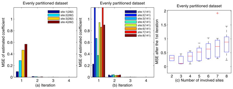
The convergence speed of evenly partitioned datasets; a) 4-site setup; b) 8-site setup; c) The MSE of each site after the 1st iteration update for n-site setups with n = 2, 3, · · ·, 8.
Finally, we studied the impact of unevenly partitioned Edinburgh dataset on the convergence speed. As shown in Fig. 5 (a), (b) and (c), we randomly selected 500, 750 and 1000 records for the first site, respectively. The remaining n − 1 sites shared the rest of the records evenly. Fig. 5 (a), (b) and (c) show, as expected, that the MSE of the first site decreases as the number of records it holds increases. As the number of records in the first site reaches 1000, the MSE drops from 2.5 to less than 10−2 within 1 iteration update. Please note that in our asynchronous EXPLORER, the inter-site information exchange starts at the 2nd iteration. This observation illustrates how the online learning works, where the model learnt from a large dataset can be used to improve the model learnt from a relatively smaller dataset. For example, in Fig. 5 (c), the models from site 2, 3, 4 learnt at the first iteration have been significantly improved at the second iteration with the information obtained from the site 1, where their MSE reduced from 100 to 10−4. However, the improvement of site 1 resulting from other sites is small, as its MSE reduction is only from the order of 10−2 to 10−4. The complexity analysis can be found in supplementary materials - Section S5.
Figure 5.

The convergence speed of unevenly partitioned dataset; a) site 1 with 500 records; b) site 1 with 750 records; c) site 1 with 1000 records.
5. Discussion and Limitation
There is currently great interest in sharing healthcare and biomedical research data to expedite discoveries that improve quality of care [46, 47, 48, 49, 29, 50, 51]. Unfortunately, healthcare institutions cannot share their data easily due to government regulations and privacy concerns. In this paper, we investigated an EXpectation Propagation LOgistic REgRession (EXPLORER) model for distributed privacy-preserving online learning. The proposed framework provides a high level guarantee for protecting sensitive information. Through experimental results, EXPLORER shows the same performance (i.e., classification accuracy, model parameter estimation) as the traditional frequentist Logistic Regression model. Practical applications of privacy-preserving predictive models can benefit from methods such as the ones employed in EXPLORER, since there it does not require re-training every time a new data point is added, and it does not need to rely on synchronous communication as its predecessor distributed logistic regression model [29].
5.1. Privacy analysis
The proposed EXPLORER provides strong privacy protection, since the exchanged statistics are always aggregated over a local population of mj −mj−1 records. This is analogous to the generalization operation used for table deidentification (i.e., k-anonymization [49]) and the aggregated statistics reduce the risk of privacy breach of individual patient. For example, when a malicious user is eavesdropping at the server side, he can only observe the difference between mh<sub>j</sub>→B (β) and mB→h<sub>j</sub>(β) at each inter-site update, where mB→h<sub>j</sub>(β) and mh<sub>j</sub>→B (β) are the messages from server node at the previous iteration and the message uploaded to server node at the current iteration, respectively. Therefore, the malicious user cannot match this aggregated difference back to each individual record in EXPLORER. A very interesting direction is to extend EXPLORER to satisfy objective privacy criteria like ε-differential privacy. We plan to investigate in future work how differential privacy can be applied.
Moreover, we introduced secured intermediate information exchange (i.e., SINE) protocol to enhance the security of the proposed EXPLORER framework, which could significantly reduce the risk of information leak due to the exchange of unprotected aggregated statistics among EXPLORER clients and server. SINE protocol is based on the modified secure sum algorithm in secure multi-parity computation, which offers a high level provable security guarantee [52].
5.2. Scalability and Communication Complexity
Since EXPLORER is working in a distributed fashion, it introduced additional communication overhead between server and clients. In general, the communication overhead between server and clients is proportional to the number of participating sites. Since we use the Normal distribution as the approximate distribution, the messages propagated between the server and the clients consist of the d dimensional mean vector β and its covariance matrix V with d(d + 1)/2 unique elements. Moreover, unlike SPARK protocol [26] with exponentially increased complexity against network size, SINE protocol is light-weighted with linearly grown complexity against network size, which offers a much better scalability.
5.3. Limitation
Although EXPLORER showed comparable performance to LR, it has some theoretical limitations: its optimization procedure is not convex, and therefore there is no guarantee for global optimal solutions. The proposed EXPLORER also introduced communication overhead, which is proportional to the number of participant sites. The convergence speed of EXPLORER depends on the partition size of each involved site.
6. Conclusions
In summary, EXPLORER offers an additional tool for privacy-preserving distributed statistical learning. We showed empirically on two relatively data sets that the results are very similar to those of ordinary logistic regression. These promising results warrant further validation in larger data sets and further refinement of the methodology. Inability to openly share (i.e., transmit) patient data without onerous processes involving pair-wise agreements between institutions may significantly slow down analyses that could produce important results for healthcare improvement and biomedical research advances. EXPLORER provides a means to mitigate this problem by relying on multi-party computation without need for extensive re-training of models, nor reliance on synchronous communications among sites.
Supplementary Material
Table 9.
Learnt model parameter β of dataset 4 (simulated correlated data with 15 covariates) using Ordinary LR and 2-site EXPLORER
| β | Ordinary LR | EXPLORER | two-sample Z test | |||
|---|---|---|---|---|---|---|
| value | std. | value | std. | Test statistic | p-value | |
| β0 | 1.988 | 0.383 | 1.924 | 0.350 | 0.673 | 0.50110 |
| β1 | −1.128 | 0.228 | −1.124 | 0.161 | −0.088 | 0.93023 |
| β2 | 1.411 | 0.136 | 1.417 | 0.119 | −0.184 | 0.85376 |
| β3 | 0.507 | 0.187 | 0.527 | 0.130 | −0.494 | 0.62096 |
| β4 | −1.160 | 0.156 | −1.199 | 0.134 | 1.024 | 0.30605 |
| β5 | 1.120 | 0.189 | 1.130 | 0.140 | −0.236 | 0.81315 |
| β6 | 2.395 | 0.113 | 2.441 | 0.107 | −1.618 | 0.10572 |
| β7 | −1.845 | 0.208 | −1.877 | 0.145 | 0.689 | 0.49098 |
| β8 | −1.330 | 0.412 | −1.338 | 0.274 | 0.089 | 0.92912 |
| β9 | 1.292 | 0.101 | 1.339 | 0.093 | −1.876 | 0.06070 |
| β10 | 1.048 | 0.179 | 1.080 | 0.148 | −0.744 | 0.45683 |
| β11 | 1.026 | 0.444 | 1.030 | 0.283 | −0.041 | 0.96726 |
| β12 | −0.278 | 0.159 | −0.289 | 0.145 | 0.269 | 0.78829 |
| β13 | −0.619 | 0.238 | −0.597 | 0.187 | −0.397 | 0.69138 |
| β14 | −3.177 | 0.142 | −3.210 | 0.134 | 0.928 | 0.35328 |
| β15 | 0.592 | 0.116 | 0.611 | 0.104 | −0.685 | 0.49331 |
Table 10.
Learnt model parameter β of dataset 5 (simulated binary data with 5 covariates) using Ordinary LR and 2-site EXPLORER
| β | Ordinary LR | EXPLORER | two-sample Z test | |||
|---|---|---|---|---|---|---|
| value | std. | value | std. | Test statistic | p-value | |
| β0 | 1.568 | 0.115 | 1.568 | 0.113 | −0.016 | 0.98758 |
| β1 | −1.443 | 0.139 | −1.432 | 0.136 | −0.300 | 0.76437 |
| β2 | 1.747 | 0.139 | 1.774 | 0.139 | −0.759 | 0.44780 |
| β3 | 1.092 | 0.166 | 1.109 | 0.164 | −0.397 | 0.69123 |
| β4 | −1.091 | 0.125 | −1.077 | 0.123 | −0.429 | 0.66817 |
| β5 | 1.444 | 0.191 | 1.472 | 0.190 | −0.569 | 0.56939 |
EXPLORER handles learning from distributed sources without sharing raw data.
EXPLORER allows client sites dynamically shift from online to offline modes.
EXPLORER offers online learning capability for efficient model update.
EXPLORER provides high estimation accuracy and strong privacy protection.
Appendix A. Expectation Propagation based Logistic Regression
Assumed-density filtering (ADF) method is a sequential technique for fast computing an approximate posterior distribution in Bayesian inference. However, the performance of ADF technique depends on the data order. Expectation propagation (EP) algorithm [53], as an extension of ADF, exploits a good approximation to the posterior by incorporating iterative refinement on the solution produced by ADF. Thus, EP is usually much more accurate than ADF. EP works by approximating each likelihood term through minimizing Kullback Leibler (KL) divergence between true posterior and approximate posterior within a tractable distribution (e.g., distributions in exponential family). Then by iteratively performing this approximation process, the approximate distribution will finally reach a fixed point [32].
In our Bayesian logistic regression problem, parameter β is associated with a Gaussian prior distribution as
Given a training dataset D = {(x1, y1), (x2, y2), · · ·, (xN, yN)}, the likelihood function for parameter β is written as
Then let us denote the true posterior distribution of β by p(β |y) ∝ p(β) Πi p(yi|β) = p(β) Πi fi(β) and approximate posterior by q(β |y) ∝ p(β)f̃i(β). It is mathematically convenient to choose a Guassian distribution for approximation term f̃i(β) such that the resulted approximate posterior will also be a Gaussian. To perform an efficient EP process, f̃i(β) can be parameterized as
The procedure to obtain the posterior approximation through EP algorithm is shown as follows [54]:
Initialize the prior distribution: f̃0(β) = N (β, 0, v0I),<lbr>set m0 = 0, V0 = v0I , where v0 is a hyper prior.
-
Initialize the term approximations f̃i(β) to 1:
set mi = 0, vi = ∞ and Zi = 1,
-
Initialize the posterior probability distribution q(β):
set mnew = m0, Vnew = V0 and Z = Z0.
-
Until all (mi, vi, Zi) converge:<lbr>for i = 1, · · ·, N :
- Remove f̃i(w) from the posterior q(β)
-
Update m new and V new according to ADF
where
- Update the approximated terms fi(w)
Appendix B. Factor Graph construction and Message passing in EXPLORER
In this section, we will introduce the details of the factor graph construction and message passing in the EXPLORER. Let us write down the factorization of the posterior distribution of each site as follows
| (B.1) |
| (B.2) |
| (B.3) |
| (B.4) |
| (B.5) |
| (B.6) |
| (B.7) |
where is a normalization constant. In the above equation, p(βj | Y1Y2Y3)is equivalent to belief b(βj) in the BP algorithm, which is captured by the variable node Bj. Therefore, in the context of factor graph and BP algorithm, we can interpret the product term as the message collected from all the factor nodes and the integral term ∫ δ (βj, β)p(β|Y2Y3) as the message sent from factor node hj. Moreover, according to the factor node update rule in BP algorithm, we can identify the delta function δ(βj, β) as the factor function and p (β | Y2Y3) as the message sent from server node B. In practice, there are many ways to select factor functions to reflect the contribution of p(βj |β). In this paper, we follow the suggestion in Loeliger [34] and choose δ(βj, β) to represent the probability p(βj |β) for mathematical convenience, because of ∫δ(βj, β)p (β | Y2Y3) dβ= p(βi|Y2Y3).
Appendix C. Model parameters learning on clinical datasets
Table C.13.
Learnt model parameter β of dataset 7 (biomarker CA-19 and CA-125) using Ordinary LR and 2-site EXPLORER
| β | Ordinary LR | EXPLORER | two-sample Z Test | |||
|---|---|---|---|---|---|---|
| value | std. | value | std. | Test statistic | p-value | |
| β0 | −1.442 | 0.243 | −1.539 | 0.252 | 1.517 | 0.12934 |
| β1 | 0.027 | 0.005 | 0.030 | 0.005 | −2.234 | 0.02547 |
| β2 | 0.016 | 0.006 | 0.019 | 0.008 | −1.481 | 0.13849 |
Table C.14.
Learnt model parameter β of dataset 8 (low birth weight study) using Ordinary LR and 2-site EXPLORER
| β | Ordinary LR | EXPLORER | two-sample Z test | |||
|---|---|---|---|---|---|---|
| value | std. | value | std. | Test statistic | p-value | |
| β0 | −0.009 | 0.346 | −0.009 | 0.308 | −0.004 | 0.99671 |
| β1 | 0.220 | 0.118 | 0.220 | 0.116 | 0.015 | 0.98831 |
| β2 | 0.462 | 0.150 | 0.453 | 0.146 | 0.224 | 0.82279 |
| β3 | 0.258 | 0.437 | 0.185 | 0.409 | 0.667 | 0.50459 |
| β4 | 0.519 | 0.116 | 0.527 | 0.115 | −0.292 | 0.77064 |
| β5 | −0.795 | 0.133 | −0.809 | 0.134 | 0.416 | 0.67711 |
| β6 | −0.856 | 0.139 | −0.862 | 0.137 | 0.152 | 0.87930 |
| β7 | 0.021 | 0.010 | 0.023 | 0.009 | −0.727 | 0.46710 |
| β8 | −0.010 | 0.002 | −0.010 | 0.001 | 1.169 | 0.24258 |
Table C.15.
Learnt model parameter β of dataset 9 (UMASS aids research) using Ordinary LR and 2-site EXPLORER
| β | Ordinary LR | EXPLORER | two-sample Z test | |||
|---|---|---|---|---|---|---|
| value | std. | value | std. | Test statistic | p-value | |
| β0 | −2.368 | 0.382 | −2.199 | 0.355 | −1.779 | 0.07527 |
| β1 | 0.050 | 0.011 | 0.046 | 0.010 | 1.482 | 0.13833 |
| β2 | 0.000 | 0.005 | −0.001 | 0.005 | 1.097 | 0.27271 |
| β3 | −0.614 | 0.142 | −0.602 | 0.141 | −0.327 | 0.74355 |
| β4 | −0.726 | 0.122 | −0.707 | 0.120 | −0.606 | 0.54419 |
| β5 | −0.072 | 0.020 | −0.079 | 0.020 | 1.434 | 0.15143 |
| β6 | 0.231 | 0.125 | 0.227 | 0.128 | 0.137 | 0.89088 |
| β7 | 0.437 | 0.096 | 0.427 | 0.096 | 0.411 | 0.68095 |
| β8 | 0.164 | 0.105 | 0.147 | 0.106 | 0.611 | 0.54091 |
Table C.16.
Learnt model parameter β of dataset 10 (mammography experience study) using Ordinary LR and 2-site EXPLORER
| β | Ordinary LR | EXPLORER | two-sample Z test | |||
|---|---|---|---|---|---|---|
| value | std. | value | std. | Test statistic | p-value | |
| β0 | −1.020 | 0.665 | −0.904 | 0.458 | −0.785 | 0.43227 |
| β1 | −0.176 | 0.251 | −0.301 | 0.209 | 2.089 | 0.03673 |
| β2 | 1.281 | 0.242 | 1.204 | 0.198 | 1.345 | 0.17877 |
| β3 | 1.732 | 0.286 | 1.643 | 0.236 | 1.320 | 0.18667 |
| β4 | −0.183 | 0.034 | −0.195 | 0.033 | 1.484 | 0.13780 |
| β5 | 1.238 | 0.182 | 1.243 | 0.180 | −0.097 | 0.92265 |
| β6 | 1.199 | 0.255 | 1.185 | 0.239 | 0.211 | 0.83267 |
| β7 | −0.671 | 0.555 | −0.621 | 0.405 | −0.400 | 0.68887 |
| β8 | −0.096 | 0.493 | −0.031 | 0.349 | −0.588 | 0.55628 |
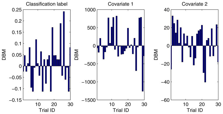
Appendix D. Heterogeneity among different EXPLORER sites
For all 2-site EXPLORER setups of datasets 3 to 11, the difference between means (DBM) of class distribution and covariates of the 2 sites has been shown in Figs. D.6 to D.14 in this section, which offers an intuitive sense about how heterogeneous these sites are.
Figure D.6.

Heterogeneity between 2 different EXPLORER sites for dataset 3 over 30 trials.
Figure D.7.

Heterogeneity between 2 different EXPLORER sites for dataset 4 over 30 trials.
Figure D.8.

Heterogeneity between 2 different EXPLORER sites for dataset 5 over 30 trials.
Figure D.9.

Heterogeneity between 2 different EXPLORER sites for dataset 6 over 30 trials.
Figure D.10.
Heterogeneity between 2 different EXPLORER sites for dataset 7 over 30 trials.
Figure D.11.

Heterogeneity between 2 different EXPLORER sites for dataset 8 over 30 trials.
Figure D.12.

Heterogeneity between 2 different EXPLORER sites for dataset 9 over 30 trials.
Figure D.13.

Heterogeneity between 2 different EXPLORER sites for dataset 10 over 30 trials.
Figure D.14.

Heterogeneity between 2 different EXPLORER sites for dataset 11 over 30 trials.
Footnotes
Publisher's Disclaimer: This is a PDF file of an unedited manuscript that has been accepted for publication. As a service to our customers we are providing this early version of the manuscript. The manuscript will undergo copyediting, typesetting, and review of the resulting proof before it is published in its final citable form. Please note that during the production process errors may be discovered which could affect the content, and all legal disclaimers that apply to the journal pertain.
Contributor Information
Shuang Wang, Email: shw070@ucsd.edu.
Xiaoqian Jiang, Email: x1jiang@ucsd.edu.
Yuan Wu, Email: y6wu@ucsd.edu.
Lijuan Cui, Email: lj.cui@ou.edu.
Samuel Cheng, Email: samuel.cheng@ou.edu.
Lucila Ohno-Machado, Email: machado@ucsd.edu.
References
- 1.Hosmer D, Lemeshow S. Applied logistic regression. Wiley-Interscience; 2000. [Google Scholar]
- 2.Boxwala A, Kim J, Grillo J, Ohno-Machado L. Using statistical and machine learning to help institutions detect suspicious access to electronic health records. J Am Med Inform Assoc. 2011;18:498–505. doi: 10.1136/amiajnl-2011-000217. [DOI] [PMC free article] [PubMed] [Google Scholar]
- 3.Ohno-Machado L. Modeling medical prognosis: survival analysis techniques. J Biomed Inform. 2001;34:428–439. doi: 10.1006/jbin.2002.1038. [DOI] [PubMed] [Google Scholar]
- 4.Kennedy R, Fraser H, McStay L, Harrison R. Early diagnosis of acute myocardial infarction using clinical and electrocardiographic data at presentation: derivation and evaluation of logistic regression models. Eur Heart J. 1996;17:1181–1191. doi: 10.1093/oxfordjournals.eurheartj.a015035. [DOI] [PubMed] [Google Scholar]
- 5.Anderson N, Edwards K. Building a chain of trust: using policy and practice to enhance trustworthy clinical data discovery and sharing. Proceedings of the 2010 Workshop on Governance of Technology, Information and Policies, ACM; Austin, Texas, USA. pp. 15–20. [Google Scholar]
- 6.Sweeney L. LIDAP-WP4. Carnegie Mellon University, Laboratory for International Data Privacy; Pittsburgh, PA: 2000. Uniqueness of simple demographics in the us population. [Google Scholar]
- 7.Ljungqvist L. A Unified Approach to Measures of Privacy in Randomized Response Models: A Utilitarian Perspective. J Am Stat Assoc. 1993;88:97–103. [Google Scholar]
- 8.Sweeney L. Others, k anonymity: A model for protecting privacy. International Journal of Uncertainty Fuzziness and Knowledge Based Systems. 2002;10:557–570. [Google Scholar]
- 9.Dwork C. Differential privacy, International Colloquium on Automata. Languages and Programming. 2006;4052:1–12. [Google Scholar]
- 10.Malin BA, Sweeney L. A secure protocol to distribute unlinkable health data. AMIA Annual Symposium proceedings, AMIA; 2005. pp. 485–489. [PMC free article] [PubMed] [Google Scholar]
- 11.Chen T, Zhong S. Privacy-preserving backpropagation neural network learning, Neural Networks. IEEE Transactions on. 2009;20:1554–1564. doi: 10.1109/TNN.2009.2026902. [DOI] [PubMed] [Google Scholar]
- 12.Yu H, Jiang X, Vaidya J. Privacy-preserving SVM using nonlinear kernels on horizontally partitioned data. Proceedings of the 2006 ACM symposium on Applied computing, SAC ’06, ACM; New York, NY, USA. 2006. pp. 603–610. [Google Scholar]
- 13.Vaidya J, Yu H, Jiang X. Privacy-preserving SVM classification. Knowledge and Information Systems. 2008;14:161–178. [Google Scholar]
- 14.Kantarcioglu M. A Survey of Privacy-Preserving Methods Across Horizontally Partitioned Data. In: Elmagarmid AK, Sheth AP, Aggarwal CC, Yu PS, editors. Privacy Preserving Data Mining, volume 34 of Advances in Database Systems. Springer US; 2008. pp. 313–335. [Google Scholar]
- 15.Vaidya J. A survey of privacy-preserving methods across vertically partitioned data. In: Aggarwal CC, Yu PS, Elmagarmid AK, editors. Privacy-Preserving Data Mining, volume 34 of The Kluwer International Series on Advances in Database Systems. Springer US; 2008. pp. 337–358. [Google Scholar]
- 16.Machanavajjhala A, Gehrke J, Kifer D, Venkitasubramaniam M. L-diversity: privacy beyond k-anonymity. Proceedings of the 22nd International Conference on Data Engineering; IEEE. 2006. pp. 1–12. [Google Scholar]
- 17.Li N, Li T, Venkatasubramanian S. t Closeness : Privacy Beyond k-Anonymity and -Diversity. Data Engineering, IEEE 23rd International Conference on, 2; IEEE. 2007. pp. 106–115. [Google Scholar]
- 18.Dwork C, McSherry F, Nissim K, Smith A. Calibrating noise to sensitivity in private data analysis. Theory of Cryptography. 2006;3876:265–284. [Google Scholar]
- 19.McSherry F, Talwar K. Mechanism Design via Differential Privacy. 48th Annual IEEE Symposium on Foundations of Computer Science (FOCS’07); IEEE, Providence, RI. 2007. pp. 94–103. [Google Scholar]
- 20.Wolfson M, Wallace S, Masca N, Rowe G, Sheehan N, Ferretti V, LaFlamme P, Tobin M, Macleod J, Little J, et al. Datashield: resolving a conflict in contemporary bioscienceperforming a pooled analysis of individual-level data without sharing the data. International journal of epidemiology. 2010;39:1372–1382. doi: 10.1093/ije/dyq111. [DOI] [PMC free article] [PubMed] [Google Scholar]
- 21.Karr A, Lin X, Sanil A, Reiter J. Analysis of integrated data without data integration. Chance. 2004;17:26–29. [Google Scholar]
- 22.Karr A, Feng J, Lin X, Sanil A, Young S, Reiter J. Secure analysis of distributed chemical databases without data integration. Journal of computer-aided molecular design. 2005;19:739–747. doi: 10.1007/s10822-005-9011-5. [DOI] [PubMed] [Google Scholar]
- 23.Fienberg S, Fulp W, Slavkovic A, Wrobel T. Privacy in Statistical Databases. Springer; secure log-linear and logistic regression analysis of distributed databases; pp. 277–290. [Google Scholar]
- 24.Karr A, Fulp W, Vera F, Young S, Lin X, Reiter J. Secure, privacy-preserving analysis of distributed databases. Technometrics. 2007;49:335–345. [Google Scholar]
- 25.Karr A. Secure statistical analysis of distributed databases, emphasizing what we don’t know. Journal of Privacy and Confidentiality. 2009;1:197–211. [Google Scholar]
- 26.El Emam K, Samet S, Arbuckle L, Tamblyn R, Earle C, Kantarcioglu M. A secure distributed logistic regression protocol for the detection of rare adverse drug events. Journal of the American Medical Informatics Association. 2012 doi: 10.1136/amiajnl-2011-000735. [DOI] [PMC free article] [PubMed] [Google Scholar]
- 27.Sparks R, Carter C, Donnelly J, OKeefe C, Duncan J, Keighley T, McAullay D. Remote access methods for exploratory data analysis and statistical modelling: Privacy-preserving analytics. Computer methods and programs in biomedicine. 2008;91:208–222. doi: 10.1016/j.cmpb.2008.04.001. [DOI] [PubMed] [Google Scholar]
- 28.Fienberg S, Nardi Y, Slavković A. Valid statistical analysis for logistic regression with multiple sources. Protecting Persons While Protecting the People. 2009:82–94. [Google Scholar]
- 29.Wu Y, Jiang X, Kim J, Ohno-Machado L. Grid binary logistic regression (GLORE): building shared models without sharing data. J Am Med Inform Assoc. 2012 doi: 10.1136/amiajnl-2012-000862. Epub ahead of print. [DOI] [PMC free article] [PubMed] [Google Scholar]
- 30.Ambrose P, Hammel J, Bhavnani S, Rubino C, Ellis-Grosse E, Drusano G. Frequentist and bayesian pharmacometric-based approaches to facilitate critically needed new antibiotic development: Overcoming lies, damn lies, and statistics. Antimicrob Agents Chemother. 2012;56:1466–1470. doi: 10.1128/AAC.01743-10. [DOI] [PMC free article] [PubMed] [Google Scholar]
- 31.Marjerison W., Jr . PhD thesis. Worcester Polytechnic Institute Thesis for Applied Statistics; 2006. Bayesian Logistic Regression with Spatial Correlation: An Application to Tennessee River Pollution. [Google Scholar]
- 32.Minka T. Microsoft Research Tech Rep MSR-TR-2005-173. 2005. Divergence measures and message passing; pp. 1–17. [Google Scholar]
- 33.Minka T. Technical Report. 2003. A comparison of numerical optimizers for logistic regression. [Google Scholar]
- 34.Loeliger H. An introduction to factor graphs, Signal Processing Magazine. IEEE. 2004;21:28–41. [Google Scholar]
- 35.Whitney A. A direct method of nonparametric measurement selection, Computers. IEEE Transactions on. 1971;100:1100–1103. [Google Scholar]
- 36.Bishop C, et al. Pattern recognition and machine learning. Vol. 4. Springer; New York: 2006. [Google Scholar]
- 37.Benaloh J. Advances in CryptologyCRYPTO86. Springer; Secret sharing homomorphisms: Keeping shares of a secret secret; pp. 251–260. [Google Scholar]
- 38.Goldreich O. Foundations of Cryptography: Volume 2, Basic Applications. 2. Cambridge University press; 2004. [Google Scholar]
- 39.Zou K. Statistical evaluation of diagnostic performance: topics in ROC analysis. Taylor & Francis; 2012. [Google Scholar]
- 40.Gaudart J, Giusiano B, Huiart L. Comparison of the performance of multi-layer perceptron and linear regression for epidemiological data. Computational statistics & data analysis. 2004;44:547–570. [Google Scholar]
- 41.Heinze G, Schemper M. A solution to the problem of separation in logistic regression. Statistics in medicine. 2002;21:2409–2419. doi: 10.1002/sim.1047. [DOI] [PubMed] [Google Scholar]
- 42.Bagley S, White H, Golomb B. Logistic regression in the medical literature:: Standards for use and reporting, with particular attention to one medical domain. Journal of clinical epidemiology. 2001;54:979–985. doi: 10.1016/s0895-4356(01)00372-9. [DOI] [PubMed] [Google Scholar]
- 43.Coding categorical variables in regression models: Dummy and effect coding. 2008. [Google Scholar]
- 44.Hosmer D, Lemesbow S. Goodness of fit tests for the multiple logistic regression model. Communications in Statistics-Theory and Methods. 1980;9:1043–1069. [Google Scholar]
- 45.Hosmer D, Hosmer T, Le Cessie S, Lemeshow S, et al. A comparison of goodness-of-fit tests for the logistic regression model. Stat Med. 1997;16:965–980. doi: 10.1002/(sici)1097-0258(19970515)16:9<965::aid-sim509>3.0.co;2-o. [DOI] [PubMed] [Google Scholar]
- 46.Wu Y, Jiang X, Ohno-Machado L. Preserving institutional privacy in distributed binary logistic regression. AMIA Annual Symposium; AMIA. 2012. accepted. [PMC free article] [PubMed] [Google Scholar]
- 47.Que J, Jiang X, Ohno-Machado L. A collaborative framework for distributed privacy-preserving support vector machine learning. AMIA Annual Symposium; AMIA. 2012. accepted. [PMC free article] [PubMed] [Google Scholar]
- 48.Jiang X, Kim J, Wu Y, Ohno-Machado L. Selecting cases for whom additional tests can improve prognosticationg. AMIA Annual Symposium; AMIA. 2012. accepted. [PMC free article] [PubMed] [Google Scholar]
- 49.Ohno-Machado L, Bafna V, Boxwala A, Chapman B, Chapman W, Chaudhuri K, Day M, Farcas C, Heintzman N, Jiang X, et al. idash: integrating data for analysis, anonymization, and sharing. J Am Med Inform Assoc. 2012;19:196–201. doi: 10.1136/amiajnl-2011-000538. [DOI] [PMC free article] [PubMed] [Google Scholar]
- 50.Jiang X, Boxwala A, El-Kareh R, Kim J, Ohno-Machado L. A patient-driven adaptive prediction technique to improve personalized risk estimation for clinical decision support. J Am Med Inform Assoc. 2012;1:e137–e144. doi: 10.1136/amiajnl-2011-000751. [DOI] [PMC free article] [PubMed] [Google Scholar]
- 51.Jiang X, Osl M, Kim J, Ohno-Machado L. Calibrating predictive model estimates to support personalized medicine. J Am Med Inform Assoc. 2012;19:263–274. doi: 10.1136/amiajnl-2011-000291. [DOI] [PMC free article] [PubMed] [Google Scholar]
- 52.Kantarcioglu M, Clifton C. Privacy-preserving distributed mining of association rules on horizontally partitioned data, Knowledge and Data Engineering. IEEE Transactions on. 2004;16:1026–1037. [Google Scholar]
- 53.Minka T. Proceedings of the Seventeenth conference on Uncertainty in artificial intelligence. Morgan Kaufmann Publishers Inc; Expectation propagation for approximate bayesian inference; pp. 362–369. [Google Scholar]
- 54.Minka T. Technical Report. 2008. Ep: A quick reference. [Google Scholar]
Associated Data
This section collects any data citations, data availability statements, or supplementary materials included in this article.