Mechanism-Based Pharmacodynamic Modeling

Abstract

Pharmacodynamic modeling is based on a quantitative integration of pharmacokinetics, pharmacological systems, and (patho-) physiological processes for understanding the intensity and time-course of drug effects on the body. Application of such models to the analysis of meaningful experimental data allows for the quantification and prediction of drug–system interactions for both therapeutic and adverse drug responses. In this chapter, commonly used mechanistic pharmacodynamic models are presented with respect to their important features, operable equations, and signature profiles. In addition, literature examples showcasing the utility of these models to adverse drug events are highlighted. Common model types that are covered include simple direct effects, biophase distribution, indirect effects, signal transduction, and irreversible effects.

1. Introduction

Pharmacodynamics represents a broad discipline that seeks to identify drug- and system-specific properties that regulate acute and long-term biological responses to drugs. The term is typically used in the context of therapeutic effects, whereas toxicology or toxicodynamics relates to adverse drug reactions. In contrast to classical conceptualizations whereby beneficial and adverse responses occur via distinct mechanisms, it is increasingly clear that diseases and both types of drug responses may emerge from perturbations of singular complex interconnected networks (1). Thus, mechanism-based pharmacody-namic models, by definition, should be multipurpose and readily adapted to understand the extent and time-course of adverse drug effects.

In the mid-1960s, Gerhard Levy was the first to mathematically demonstrate a link between pharmacokinetics (factors controlling drug exposure) and the rate of decline of in vivo pharmacological responses (2, 3). Since that landmark discovery, pharmacodynamic modeling has evolved into a quantitative field that aims to mathematically characterize the temporal aspects of drug effects via emulating mechanisms of action (4). The application of mathematical models to describe drug–system interactions allows for the quantification and prediction of subsequent interactions within the system. The major goals of pharmacodynamic modeling are to integrate known system components, functions, and constraints, generate and test competing hypotheses of drug mechanisms and system responses under new conditions, and estimate system-specific parameters that may be inaccessible (5). These models are applicable to a wide range of disciplines within the biological sciences including pharmacology and toxicology, wherein there is a critical need to understand and predict desired and adverse responses to xenobiotic exposure, which together define the clinical utility or therapeutic index.

The main objectives of this chapter are to illustrate commonly used mechanistic pharmacodynamic models, providing important model features, operable equations, and signature profiles, as well as examples of the application of these models to the analysis of drug-induced adverse reactions.

2. Modeling Requirements

Useful pharmacodynamic models are based on plausible mathematical and pharmacological exposure–response relationships. Basic model components encompassing a range of pharmacodynamic systems are illustrated in Fig. 1. For most drug effects, both pharmacological mechanisms, often characterized by sensitivity-grounded capacity-limited effector units, and physiological turnover processes need to be integrated with drug disposition when constructing a PK/PD model.

Fig. 1.

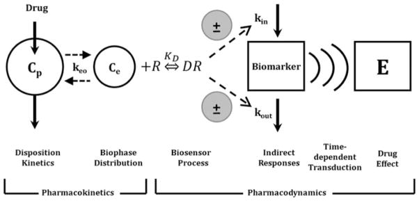
Basic components of pharmacodynamic models. The time-course of drug concentrations in a relevant biological fluid (e.g., plasma, C_p) or the biophase (C_e) is characterized by a mathematical function that serves to drive PD models. The biosensor process involves the interaction between the drug and the pharmacologic target (R), and may be described using various receptor-occupancy models, may require equations that consider the kinetics of the drug–receptor complex formation and dissociation, or may encompass irreversible drug–target interactions. Many drugs act via indirect mechanisms and the biosensor process may serve to stimulate or inhibit the production (k_in) or loss (k_out) of endogenous mediators. These altered mediators may not represent the final observed drug effect (E) and further time-dependent transduction processes may occur, thus requiring additional modeling components. System complexities such as drug interactions, functional adaptation, changes with pathophysiology, and other factors may play a role in regulating drug effects after acute and long-term drug exposure (adapted from ref. 33).

The construction and evaluation of relevant PK/PD models require suitable pharmacokinetic data, an appreciation for molecular and cellular mechanisms of pharmacological/toxicological responses, and a range of quantitative experimental measurements of meaningful biomarkers within the causal pathway between drug–target interactions and clinical effects. Good experimental designs are essential to ensure that sensitive and reproducible data are collected. These data should cover a reasonably wide dose/concentration range and appropriate study duration to ascertain net drug exposure and the ultimate fate of the biomarkers or outcomes under investigation. A wide range of systemic drug concentrations is also typically required for the accurate and precise estimation of pharmacodynamic parameters. Typically studies should involve a minimum of two to three doses to adequately estimate the nonlinear parameters of most pharmacodynamic models with simultaneous collection of concentration and response data. For more complex systems (and therefore models), more extensive datasets are required as these models typically incorporate multiple nonlinear processes and pharmacodynamic endpoints. Models are typically defined using ordinary differential equations and include both drug- and system-specific parameters. This separation of terms provides a platform for translational research, whereby relationships with in vitro bioassays and preclinical experiments can be identified.

Once a structural model has been selected, unknown parameter values can be estimated using nonlinear regression techniques. It is beyond the scope of this chapter to review the vast array of software programs and algorithms available, and the best tool and approach will often be defined by the characteristics of the experimental data, the familiarity of the end user with specific programs, and the goals and objectives of the analysis. The type of model (e.g., data-driven versus systems models), the nature of the biomarker (e.g., continuous versus categorical), the degree of inter-subject variability, and complexities within a dataset (e.g., missing variables, data above or below a limit of quantification, and availability of covariates) are just a few considerations when selecting an approach to develop and qualify PK/PD models.

3. Practical Modeling Approaches

The first steps in any modeling endeavor are to define the objectives of the analysis and to perform a careful graphical analysis of raw data. Both efforts should facilitate selection of appropriate techniques and conditions for model construction and evaluation. A good graphical analysis (along with a priori knowledge of drug mechanisms) may be used to narrow down the number of structural models being considered as a base model and also help in calculating initial parameter estimates. Despite progress in computational algorithms, good initial parameter estimates can reduce the likelihood of falling into local minima and can also be used as a reality check when compared to final parameter estimates or literature reported values. Next, an appropriate drug/toxin pharmacokinetic/toxicokinetic function is derived from fitting a model to concentration–time profiles in relevant biological fluids. Depending on the complexity of the pharmacodynamic model/system, the pharmacokinetic model and associated parameters are often fixed to serve as a driving function for the pharmacodynamic model relating drug exposure to pharmacological/toxicological effects. Although simultaneous PK/PD modeling is desirable, this can still be a formidable challenge for complex models. Objective model-fitting criteria (e.g., diagnostic and goodness-of-fit plots) are frequently compared to select a final model, and a variety of techniques are available to verify or qualify models, which can range in complexity depending on the modeling approach (e.g., population versus pooled data). Ideally, an external dataset, not used in the construction of the model, could be used to determine whether the model is generalizable; however, internal validation steps are far more common as most model-builders will attempt to incorporate all available experimental data. In any event, final models should reasonably recapitulate the data used to derive the model, generate new insights and testable hypotheses of factors controlling drug responses, and provide guidance for subsequent decisions in drug discovery, development, and pharmacotherapy. Subsequent sections will highlight commonly used pharmacodynamic models with increasing degrees of complexity, as well as provide literature examples on the application of such models to the analysis of drug-induced adverse events.

3.1. Simple Direct Effect Models

The Hill equation assumes that drugs effects (E) are directly proportional to receptor occupancy (i.e., linear transduction), assumes that plasma drug concentrations are in rapid equilibrium with the effect site, and represents a fundamental pharmacodynamic relationship (6):

$$E=E_0\pm \frac{E_{\mathit{max}}\times C_{\text{p}}}{{\text{EC}}_{50}+C_{\text{p}}}.$$ (1)

This equation, also known as the E_max model, describes the concentration–effect relationship in terms of a baseline effect or E₀ (if applicable), the maximum possible effect (E_max), and the drug concentration producing half maximal effect (EC₅₀). These parameters can be visualized easily from a plot of effect versus log- concentration where E_max is the plateau at relatively high concentrations and EC₅₀ is the drug concentration associated with E = 0.5 × E_max. Signature temporal profiles for simple direct effects for a compound with monoexponential disposition are shown in Fig. 2. The effect versus time curves appear saturated at high dose levels, decline linearly and in parallel over a range of doses, and the peak response time corresponds with the time of peak drug concentrations.

Fig. 2.

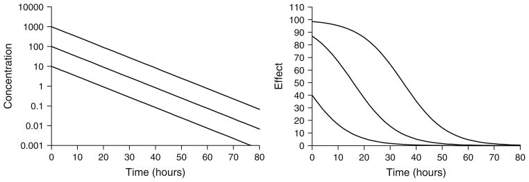
Simulated drug concentrations (left) and response curves (right) using a simple E_max model (Eq. 1). Drug concentrations follow monoexponential disposition: C_p = C^oe^(−kt). C^o was set to 10, 100, or 1,000 units to achieve increasing dose levels. Parameter values were k = 0.12/h, E_max = 100 units, and EC₅₀ = 15 units.

If a sufficient range of concentrations is not achieved, or cannot be obtained for safety reasons, the Hill equation can be reduced to simpler functions. For concentrations significantly less than the EC₅₀, C_p in the denominator of Eq. 1 is negligible, and drug effect is directly proportional to plasma drug concentrations:

$$E=E_{\text{o}}\pm S\times C_{\text{p}},$$ (2)

with S as the slope of the relationship. When the effect is between 20 and 80% maximal, according to Eq. 1, the effect is directly proportional to the log of drug concentrations:

$$E=E_0\pm mlog{C}_{\text{p}},$$ (3)

with m as the slope of the relationship. These reduced functions are only valid within certain ranges of drug concentrations relative to drug potency, and hence cannot be extrapolated to identify the maximal pharmacodynamic effect of a compound.

The full Hill equation, or sigmoid E_max model, incorporates a curve-fitting parameter, γ, which describes the steepness of the concentration–effect relationship:

$$E=E_0\pm \frac{E_{\mathit{max}}\times C_{\text{p}}^{\gamma }}{{\text{EC}}_{50}^{\gamma }+C_{\text{p}}^{\gamma }}.$$ (4)

Initial estimates for this parameter can be determined using the linear slope of the effect versus log-concentration plot:

$$m=\frac{E_{max}\times \gamma }{4}.$$ (5)

As the Hill coefficient increases from 1 to 5, the concentration–effect relationship becomes less graded, and values of 5 tend to result in quantal or all-or-none types of effects. In contrast, values less than 1 produce very shallow slopes.

Simple direct effect models have been utilized to characterize the adverse effects of a number of drugs. Arrhythmias may occur as a side effect of cardiac and noncardiac therapies, and an increasing number of studies are conducted with QTc intervals as the toxico-dynamic endpoint. QTc prolongation in response to citalopram (7) and tacrolimus (8) has been modeled using a simple E_max function (Fig. 3). The simple E_max model incorporating baseline measurements of the dynamic endpoints was also used to model the cardiovascular toxicity of cocaine administration (9). The model reasonably described the effects of cocaine on multiple endpoints including heart rate and systolic and diastolic blood pressure. Both the E_max and sigmoid E_max models were evaluated for describing methemoglobin formation from dapsone metabolites (10); however, fitting criteria were not evaluated to select the best model.

Fig. 3.

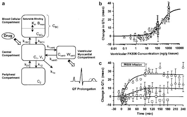
Direct effect model of tacrolimus-induced changes of QTc intervals in guinea pigs. The pharmacokinetic model includes both plasma and ventricular myocardial drug concentrations (a), and the latter are associated with changes in QTc according to Eq. 4 (b). The PK/PD relationship results in the time-course of changes in QTc (c). Reprinted from ref. 8 with permission from Springer.

3.2. Biophase Distribution

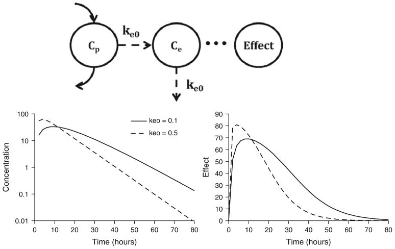
In many cases, the in vivo pharmacological effects will lag behind plasma drug concentrations. This results in the phenomenon of hysteresis, or a temporal disconnect in effect versus concentration plots. Distribution of drug to its site of action might represent a rate-limiting process that may account for the delay in drug effect. The term “biophase” was coined by Furchgott (11) to describe the drug site of action, and a mathematical approach to linking plasma concentrations and drug effect through a hypothetical effect compartment was popularized by Sheiner and colleagues (12) (Fig. 4, top panel). Plasma drug concentrations are described using an appropriate pharmacokinetic model, and the rate of change of drug concentrations at the biophase (C_e) is defined as

Fig. 4.

Biophase model structure (top panel) and signature profiles for drug concentrations at the biophase (left bottom panel) and pharmacological effects (right bottom panel). Response curves were simulated using Eqs. 1 and 6 driven by drug concentrations following monoexponential disposition: C_p = C^oe^(−kt). C^o was set to 100 units. Parameter values were k = 0.12/h, k_eo = 0.1 or 0.5/h, E_max = 100 units, and EC₅₀ = 15 units.

$$\frac{{\text{d}C}_{\text{e}}}{\text{d}t}=k_{\text{eo}}\times C_{\text{p}}-k_{\text{eo}}\times C_{\text{e}},$$ (6)

with k_eo as a first-order distribution rate constant. Although separate rate constants for production and loss were first proposed, they are often set as the same term (k_eo) for identifiability purposes. The amount of drug moving into and out of this compartment is assumed to be negligible, and therefore does not influence the pharmacokinetics of the drug. Biophase distribution is combined with Eq. 1 or 4, with C_e from Eq. 6 replacing C_p to drive the pharmacological effect. Figure 4 (bottom panels) illustrates the signature profile of the biophase model (i.e., biophase concentration and effect profiles) for a drug exhibiting monoexponential disposition. Peak drug effects are delayed relative to peak plasma concentrations; however, the time to peak effect is observed at the same time, independent of the dose level. The time to peak drug effect is related to k_eo, with smaller values resulting in later peak effects. Furthermore, for large dose levels, the slope of the decline of effect is linear and parallel between 20 and 80% of the maximum effect. Estimation of biophase model parameters can be done sequentially by fitting the pharmacokinetics and then fitting the biophase and pharmacodynamic parameters, or by simultaneously fitting all terms.

The biophase model is only suitable for describing delayed responses due to drug distribution. As it was the first approach for describing such delayed drug responses, it has been commonly misapplied to describe systems in which the rate-limiting step is unrelated to drug distribution, resulting in poor fitting and/or unrealistic parameter values.

The biophase model was implemented for describing buprenorphine-induced respiratory depression in rats (13), and the clinical prediction of transient increases in blood pressure (14). Yassen and colleagues (13) utilized biophase distribution combined with a sigmoidal E_max model to characterize changes in ventilation following a range of dose levels of buprenorphine. In contrast, increases in blood pressure resulting from a drug in clinical development were described using the biophase model coupled with a more complex pharmacodynamic relationship incorporating changes from a blood pressure set point (14).

3.3. Indirect Response Models

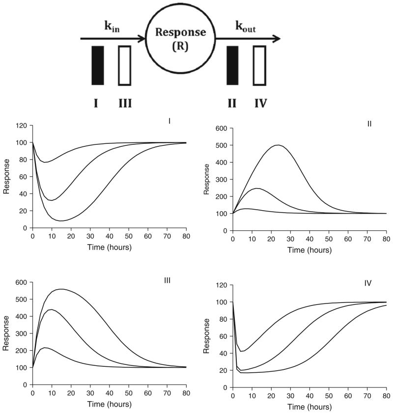
Indirect response models represent a highly useful class of models wherein reversible drug–receptor interactions serve to alter the natural production or loss of biomarker response variables. A model reflecting inhibition of production was first utilized to characterize prothrombin activity in blood after oral warfarin administration (15). Dayneka and colleagues (16) were the first to formally propose four basic indirect response models whose structures are detailed in Fig. 5 (top panel). These models have been used to investigate the pharmacodynamics of a wide range of drug effects, and their mathematical properties have been well characterized (17, 18). The four basic models include inhibition of production (Model I) or dissipation (Model II) of response or stimulation of production (Model III) or dissipation of response (Model IV), and are defined by the following differential equations:

Fig. 5.

Indirect response model structure (top panel) and signature profiles for the four basic indirect response models (middle and bottom panels). Response curves were simulated using Eqs. 7, 8, 9, and 10 driven by drug concentrations following monoexponential disposition: C_p = C^oe^(−kt). C^o was set to 10, 100, or 1,000 units to achieve increasing doses. Parameter values were k = 0.12/h, I_max = 1 unit (Models I and II), S_max = 10 units (Models III and IV), EC₅₀ = 15 units, k_out = 0.25/h, and R^o = 100 units (k_in = R^ok_out).

3.3.1. Model I

$$\frac{\text{d}R}{\text{d}t}=k_{\text{in}}\left(1-\frac{I_{max}\times C_{\text{p}}}{{\text{IC}}_{50}+C_{\text{p}}}\right)-k_{\text{out}}\times R.$$ (7)

3.3.2. Model II

$$\frac{\text{d}R}{\text{d}t}=k_{\text{in}}-k_{\text{out}}\left(1-\frac{I_{max}\times C_{\text{p}}}{{\text{IC}}_{50}+C_{\text{p}}}\right)R.$$ (8)

3.3.3. Model III

$$\frac{\text{d}R}{\text{d}t}=k_{\text{in}}\left(1+\frac{S_{\mathit{max}}\times C_{\text{p}}}{{\text{SC}}_{50}+C_{\text{p}}}\right)-k_{\text{out}}\times R.$$ (9)

3.3.4. Model IV

$$\frac{\text{d}R}{\text{d}t}=k_{\text{in}}-k_{\text{out}}\left(1+\frac{S_{max}\times C_{\text{p}}}{{\text{SC}}_{50}+C_{\text{p}}}\right)R,$$ (10)

where k_in is a zero-order production rate constant, k_out is a first-order elimination rate constant, I_max and S_max are defined as the maximum fractional factors of inhibition (0 < I_max ≤ 1) or stimulation (S_max > 0), and IC₅₀ and SC₅₀ are defined as the EC₅₀. Initial parameter estimates can be obtained from a graphical analysis of PK/PD data as previously described (17, 18). Signature profiles for these models in response to increasing dose levels are shown in Fig. 5 (middle and bottom panels). Interestingly, the time to peak responses are dose dependent, occurring at later times as the dose level is increased. This phenomenon is easily explained as the inhibition or stimulation effect will continue for larger doses, as drug remains above the EC₅₀ for longer times. The initial condition for all models (R₀) is k_in/k_out which may be set constant or fitted as a parameter during model development. Ideally, a number of measurements should be obtained prior to drug administration to assess baseline conditions. Based on the determinants of R₀, typically the baseline and one of the turnover parameters are estimated, and the remaining rate constant is calculated as a function of the two estimated terms. This reduces the number of parameters to be estimated and maintains system stationarity.

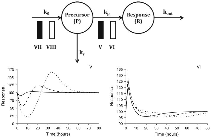
The basic indirect response models can be extended to incorporate a precursor compartment (P). The following equations represent a general set of precursor-dependent indirect response models (Fig. 6, top panel) that were developed and characterized by Sharma and colleagues (19):

$$\frac{\text{d}P}{\text{d}t}=k_{\text{o}}\{1\pm H_1(C_{\text{p}})\}-(k_{\text{s}}+k_{\text{p}}\{1\pm H_2(C_{\text{p}})\})P,$$ (11)

$$\frac{\text{d}R}{\text{d}t}=k_{\text{p}}\{1\pm H_2(C_{\text{p}})\}\times P-k_{\text{out}}\times R,$$ (12)

where k₀ represents the zero-order rate constant for precursor production, k_p is a first-order rate constant for production of the response variable, and k_out is the first-order rate constant for dissipation of response. H₁ and H₂ represent the inhibition or stimulation of precursor production or production of response and are analogous to the I_max and S_max functions presented in Eqs. 7 through 10. Stimulation or inhibition of k_p is more commonly observed than alterations in the production of precursor. The signature profiles for models V and VI are shown in Fig. 6 (bottom panels) and clearly demonstrate the rebound effect as drug washes out of the system. The data requirements for these models are similar to the basic indirect response models; however, sufficient data are needed to adequately capture baseline, maximum, and rebound effects, as well as the eventual gradual return to baseline conditions. Responses should be evaluated for two to three doses, with a sufficiently large dose to capture the maximum effect. The response measurements for the large dose should be used to determine initial parameter estimates followed by simultaneous fitting of all response data. Initial parameter estimates should be derived as previously described (19).

Fig. 6.

Multiple compartment indirect response models (top panel) and signature profiles for Models V and VI (bottom panel). Response curves were simulated using Eqs. 11 and 12 driven by drug concentrations following monoexponential disposition: C_p = C^oe^(−kt). C^o was set to 10, 100, or 1,000 units to achieve increasing doses. Parameter values were k = 0.12/h, I_max = 1 unit, S_max = 10 units, EC₅₀ = 15 units, k_o = 25 unit/h, k_p = 0.5/h, and k_out = 0.25/h.

Indirect response models have been utilized to describe the pharmacodynamic effects of a wide range of compounds that alter the natural bioflux or turnover of endogenous substances or functions. A basic indirect response model for erythropoietin was extended to include multiple-compartments for describing the turnover of red blood cells and carboplatin-induced anemia (20).

This model nicely illustrates the development of a more complex model based on indirect mechanisms of drug action to simultaneously describe multiple in vivo processes.

3.4. Signal Transduction Models

Substantial time-delays in the observed pharmacodynamic response may result from multiple time-dependent steps occurring between drug–receptor binding and the ultimate pharmacological response. A transit compartment approach can be utilized to describe a lag between drug concentration and observed effects owing to time-dependent signal transduction (21, 22). Assuming rapid receptor binding, the following differential equation describes the rate of change of the initial transit compartment (M₁):

$$\frac{{\text{d}M}_1}{\text{d}t}=\frac{1}{\tau }\left(\frac{E_{\mathit{max}}\times C_{\text{p}}}{{\text{EC}}_{50}+C_{\text{p}}}-M_1\right),$$ (13)

wherein the E_max model describes the drug–receptor interaction, and τ is the mean transit time through this compartment. Subsequent transit compartments may be added, and a general equation for the ith compartment can be defined as

$$\frac{{\text{d}M}_i}{\text{d}t}=\frac{1}{\tau }(M_{i-1}-M_i).$$ (14)

Later compartments will show a clear delay in the onset of response as well as substantial delays in achieving the maximum effect. Model development for signal transduction systems typically includes evaluating varied numbers of transit compartments and values for τ to determine the combination that best describes the data.

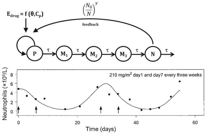
Chemotherapy-induced myelosuppression represents a classic example of the use of a transit compartment modeling to describe this adverse reaction to numerous chemotherapeutic agents (Fig. 7, top panel). The structural model was proposed by Friberg and colleagues (23) to describe myelosuppression induced by irinotecan, vinflunine (Fig. 7, bottom panel), and 2′-deoxy-2′-methylidenecyti-dine for a range of dose levels and various dosing regimens. This same structural model has been used to describe indisulam-induced mye-losuppression (24), as well as the drug–drug interactions between indisulam and capecitabine (25), and pemetrexed and BI2536 (26).

Fig. 7.

Transit-compartment model of myelosuppression (top panel) including a proliferating progenitor pool (P), three transit compartments (M_i), and a plasma neutrophil compartment (N). Drug effect is driven by plasma drug concentration (C_p) and pharmacodynamic parameters (θ). An adaptive feedback function on the proliferation rate constant is governed by the ratio of initial neutrophils to current neutrophil count, raised to a power coefficient (γ). The time-course of neutrophils following vinflunine administration (arrows in bottom panel). Reprinted from ref. 23 with permission from the American Society of Clinical Oncology.

3.5. Irreversible Effect Models

A wide range of compounds, including anticancer drugs, antimicrobial drugs, and enzyme inhibitors, elicit irreversible effects. A basic model for describing irreversible effects was developed by Jusko and includes simple cell killing (27):

$$\frac{\text{d}R}{\text{d}t}=-k\times C\times R,$$ (15)

where R represents cells or receptors, C is either C_p or C_e, and k is a second-order cell-kill rate constant. The initial condition for this equation is the initial number of cells present within the system (R₀) often represented as a survival fraction. This approach is only applicable for non-proliferating cell populations, but may be extended to incorporate cell growth (27):

$$\frac{\text{d}R}{\text{d}t}=k_s\times R-k\times C\times R,$$ (16)

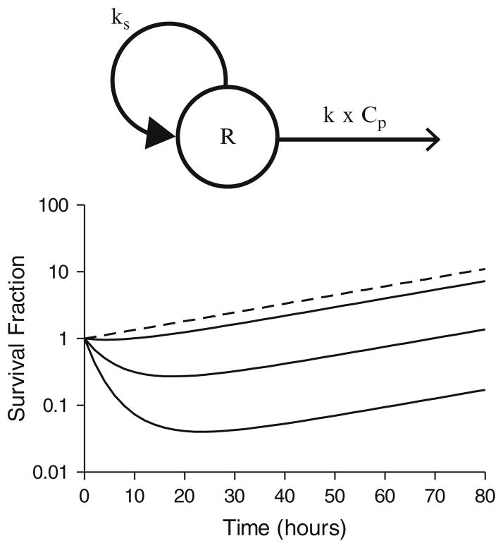
with k_s as an apparent first-order growth rate for proliferating cell populations, such as malignant cells or bacteria. This growth rate constant represents the net combination of natural growth and degradation of the cellular population, and its initial estimate can be determined from a control- or nondrug-treated cell population. The model diagram and corresponding signature profiles are shown in Fig. 8. The initial slope of the log survival fraction versus time curve out to time, t, and the plasma drug AUC_(0–t) can be used to obtain an initial estimate for k (k = −ln S_Ft/AUC_(0–t)), and the initial condition for Eq. 16 is the total cell population at time zero. In contrast to simple cell killing, the effect–time profiles are characterized by an initial cell kill phase, followed by an exponential growth phase, once drug concentrations are below an effective concentration (Fig. 8, bottom panel). Clearly the control group is needed to properly characterize the exponential growth rate constant in the untreated cell population.

Fig. 8.

Structural model for irreversible effects (top panel) and signature profiles for irreversible effect model with a proliferating cell population (bottom panel). Response curves were simulated using Eq. 16 driven by drug concentrations following monoexponential disposition: C_p = C^oe^(−kt). C^o was set to 0, 10, 100, or 1,000 units to achieve a control population and increasing dose levels. Pharmacokinetic parameter was k = 0.12/h. Pharmacodynamic parameters were k = 0.0005 units/h, k_s = 0.03/h.

The irreversible effect model can also be adapted to include the turnover or production and loss of a biomarker:

$$\frac{\text{d}R}{\text{d}t}=k_{\text{in}}-k_{\text{out}}R-k\times C\times R.$$ (17)

The initial condition for this model is the same as basic indirect responses or k_in/k_out. The signature profiles for this model are similar to the profiles for indirect response models I and IV (Fig. 5). It is important to understand the mechanism of action of the response that you are evaluating in order to determine which model should be utilized.

Irreversible effect models are commonly used to describe the cell killing action of chemotherapeutic agents and anti-infectives. This model was also applied to evaluate the formation of methe-moglobin following the administration of a range of antimalarial agents (28). The final model characterized methemoglobin production resulting from the formation of an active drug metabolite.

3.6. More Complex Models

The main focus of this chapter was the introduction of commonly used mechanistic pharmacodynamic models that can be readily applied to toxicokinetics and dynamics. However, a number of mechanistic processes may be required to adequately describe the drug–system interactions under investigation. Slow receptor binding, tolerance phenomenon, drug interactions, opposing drug effects, and disease progression may add additional complexities to the analysis of toxicodynamic data. For example, Houze and colleagues (29) evaluated paraoxon-induced respiratory toxicity and its reversal with pralidoxime (PRX) administration in rats via the combination of multiple pharmacodynamic modeling components. Initially, the time-course of paraoxon inactivation of in vitro whole blood cholinesterase (WBChE) was modeled based on enzyme inactivation:

$$\frac{{\text{d}E}_{\text{A}}}{\text{d}t}=-\left(\frac{{kC}_{\text{PO}}}{{\text{EC}}_{50,\text{PO}}+C_{\text{PO}}}\right)E_{\text{A}}+k_r{E}_{\text{I}},$$ (18)

where E_A is active enzyme, k is the maximal rate constant of enzyme inactivation, C_PO is paraoxon concentration, EC_50,PO is the concentration of paraoxon that produces 50% of k, k_r is a first-order reactivation rate constant, and E_I is the inactive enzyme pool. The rate of change of the inactive enzyme (E_I) was defined as

$$\frac{{\text{d}E}_I}{\text{d}t}=\left(\frac{{kC}_{\text{PO}}}{{\text{EC}}_{50,\text{PO}}+C_{\text{PO}}}\right)E_A-(k_r+k_{\text{age}})E_{\text{I}},$$ (19)

where k_age is a first-order rate constant of aging of inactive enzyme. The reactivation of this in vitro system by PRX was modeled as an indirect response, and Eqs. 18 and 19 were updated accordingly:

$$\frac{{\text{d}E}_{\text{A}}}{\text{d}t}=-\left(\frac{{kC}_{\text{PO}}}{{\text{EC}}_{50,\text{PO}}+C_{\text{PO}}}\right)E_{\text{A}}+k_{\text{r}}\left(1+\frac{E_{max}{C}_{\text{PRX}}^h}{{\text{EC}}_{50,\text{PRX}}^h+C_{\text{PRX}}^h}\right)E_{\text{I}}$$ (20)

$$\frac{{\text{d}E}_{\text{I}}}{\text{d}t}=\left(\frac{{kC}_{\text{PO}}}{{\text{EC}}_{50,\text{PO}}+C_{\text{PO}}}\right)E_{\text{A}}-k_{\text{r}}\left(1+\frac{E_{max}{C}_{\text{PRX}}^h}{{\text{EC}}_{50,\text{PRX}}^h+C_{\text{PRX}}^h}\right)E_{\text{I}}-(k_{\text{age}}{E}_{\text{I}}).$$ (21)

Interestingly, the estimated potency of PRX was in agreement with an empirical literature estimate. For the in vivo dynamics, a fixed pharmacokinetic function for PRX was introduced, and an empirical function was used to describe paraoxon-induced enzyme inactivation, as plasma concentrations were unavailable. The estimated parameters from the in vitro analysis were fixed (not identi-fiable from in vivo data only), and the toxicodynamic biomarker, expiratory time (T_E), was linked to apparent active enzyme (E_A) according to the following nonlinear transfer function:

$$T_{\text{E}}=T_{\text{E}}^0+\frac{E_{max,T_{\text{E}}}{\left(\frac{E_0}{E_{\text{A}}}-1\right)}^n}{E_{50}^n+{\left(\frac{E_0}{E_{\text{A}}}-1\right)}^n},$$ (22)

where $T_{\text{E}}^0$ is the baseline expiratory time, E_{max, TE} is the maximal increase in T_E, E₀ is the baseline active enzyme (1 or 100%), E₅₀ is the corrected enzyme ratio resulting in 50% of E_{max, TE}, and n is a sigmoidicity coefficient. Expiratory profiles and the transient antidotal effect of PRX were described well, and this analysis highlights the integration of several basic modeling approaches described in this chapter. Further, the coupling of in vitro enzyme and in vivo toxicodynamic data demonstrates the versatility and multi-scale nature of the model.

An additional theoretical example of mechanism-based analysis of drug interactions was presented by Earp and colleagues (30), who examined drug interactions utilizing indirect response models. These more complex models typically consider multiple pharmaco-dynamic endpoints which require individual data sets and stepwise analysis for each endpoint. A corticosteroid model which considers mRNA dynamics of the glucocorticoid receptor and hepatic tyro-sine aminotransferase mRNA and activity is an example of simultaneously characterizing multiple pharmacodynamic endpoints using an integration of basic modeling components (31).

The majority of mechanism-based pharmacodynamic models describe continuous physiological response variables. However, models are available for evaluating noncontinuous outcomes, such as the probability of a specific event occurring. Such responses are often more clinically relevant, and more research is needed to combine continuous mechanistic PK/PD models with clinical outcomes data. One example is the prediction of enoxaparin-induced bleeding events in patients undergoing various therapeutic dosing regimens (32). A population proportional-odds model was developed to predict the severity of bleeding event on an ordinal scale of 1–3 (32).

4. Prospectus

The future of mechanism-based pharmacodynamic modeling for both therapeutic and adverse drug responses is promising for model-based drug development and therapeutics, and many of the basic modeling concepts in this chapter will likely continue to represent key building components in more complex systems models. A diverse array of models is available with a minimal number of identifiable parameters to mimic mechanisms and the time-course of therapeutic and adverse drug effects. However, new methodologies will be needed to evolve these models further into translational platforms and prospectively predictive models of drug efficacy and safety. Network-based systems pharmacology models have shown utility for understanding drug-induced adverse events (1). Further research is needed to identify practical techniques for bridging systems pharmacology and in vivo PK/PD models to anticipate the clinical utility of new chemical entities from first principles.

References

- 1.Berger SI, Iyengar R. Role of systems pharmacology in understanding drug adverse events. Wiley Interdiscip Rev Syst Biol Med. 2011;3:129–135. doi: 10.1002/wsbm.114. [DOI] [PMC free article] [PubMed] [Google Scholar]
- 2.Levy G. Relationship between elimination rate of drugs and rate of decline of their pharmacologic effects. J Pharm Sci. 1964;53:342–343. doi: 10.1002/jps.2600530325. [DOI] [PubMed] [Google Scholar]
- 3.Levy G. Kinetics of pharmacologic effects. Clin Pharmacol Ther. 1966;7:362–372. doi: 10.1002/cpt196673362. [DOI] [PubMed] [Google Scholar]
- 4.Mager DE, Wyska E, Jusko WJ. Diversity of mechanism-based pharmacodynamic models. Drug Metab Dispos. 2003;31:510–518. doi: 10.1124/dmd.31.5.510. [DOI] [PubMed] [Google Scholar]
- 5.Yates FE. On the mathematical modeling of biological systems: a qualified ‘pro’. In: Vernberg FJ, editor. Physiological adaptation to the environment. Intext Educational Publishers; New York: 1975. [Google Scholar]
- 6.Wagner JG. Kinetics of pharmacologic response. I. Proposed relationships between response and drug concentration in the intact animal and man. J Theor Biol. 1968;20:173–201. doi: 10.1016/0022-5193(68)90188-4. [DOI] [PubMed] [Google Scholar]
- 7.Friberg LE, Isbister GK, Hackett LP, Duffull SB. The population pharmacokinetics of citalopram after deliberate self-poisoning: a Bayesian approach. J Pharmacokinet Pharma-codyn. 2005;32:571–605. doi: 10.1007/s10928-005-0022-6. [DOI] [PubMed] [Google Scholar]
- 8.Minematsu T, Ohtani H, Yamada Y, Sawada Y, Sato H, Iga T. Quantitative relationship between myocardial concentration of tacroli-mus and QT prolongation in guinea pigs: phar-macokinetic/pharmacodynamic model incorporating a site of adverse effect. J Pharmacokinet Pharmacodyn. 2001;28:533–554. doi: 10.1023/a:1014460404352. [DOI] [PubMed] [Google Scholar]
- 9.Laizure SC, Parker RB. Pharmacody-namic evaluation of the cardiovascular effects after the coadministration of cocaine and ethanol. Drug Metab Dispos. 2009;37:310–314. doi: 10.1124/dmd.108.023531. [DOI] [PMC free article] [PubMed] [Google Scholar]
- 10.Vage C, Saab N, Woster PM, Svensson CK. Dapsone-induced hematologic toxicity: comparison of the methemoglobin-forming ability of hydroxylamine metabolites of dapsone in rat and human blood. Toxicol Appl Pharmacol. 1994;129:309–316. doi: 10.1006/taap.1994.1255. [DOI] [PubMed] [Google Scholar]
- 11.Furchgott RF. The pharmacology of vascular smooth muscle. Pharmacol Rev. 1955;7:183–265. [PubMed] [Google Scholar]
- 12.Sheiner LB, Stanski DR, Vozeh S, Miller RD, Ham J. Simultaneous modeling of phar-macokinetics and pharmacodynamics: application to d-tubocurarine. Clin Pharmacol Ther. 1979;25:358–371. doi: 10.1002/cpt1979253358. [DOI] [PubMed] [Google Scholar]
- 13.Yassen A, Kan J, Olofsen E, Suidgeest E, Dahan A, Danhof M. Pharmacokinetic-pharmacodynamic modeling of the respiratory depressant effect of norbuprenorphine in rats. J Pharmacol Exp Ther. 2007;321:598–607. doi: 10.1124/jpet.106.115972. [DOI] [PubMed] [Google Scholar]
- 14.Stroh M, Addy C, Wu Y, Stoch SA, Pourkavoos N, Groff M, Xu Y, Wagner J, Gottesdiener K, Shadle C, Wang H, Manser K, Winchell GA, Stone JA. Model-based decision making in early clinical development: minimizing the impact of a blood pressure adverse event. AAPS J. 2009;11:99–108. doi: 10.1208/s12248-009-9083-6. [DOI] [PMC free article] [PubMed] [Google Scholar]
- 15.Nagashima R, O’Reilly RA, Levy G. Kinetics of pharmacologic effects in man: the anticoagulant action of warfarin. Clin Pharma-col Ther. 1969;10:22–35. doi: 10.1002/cpt196910122. [DOI] [PubMed] [Google Scholar]
- 16.Dayneka NL, Garg V, Jusko WJ. Comparison of four basic models of indirect phar-macodynamic responses. J Pharmacokinet Biopharm. 1993;21:457–478. doi: 10.1007/BF01061691. [DOI] [PMC free article] [PubMed] [Google Scholar]
- 17.Jusko WJ, Ko HC. Physiologic indirect response models characterize diverse types of pharmacodynamic effects. Clin Pharmacol Ther. 1994;56:406–419. doi: 10.1038/clpt.1994.155. [DOI] [PubMed] [Google Scholar]
- 18.Sharma A, Jusko WJ. Characteristics of indirect pharmacodynamic models and applications to clinical drug responses. Br J Clin Phar-macol. 1998;45:229–239. doi: 10.1046/j.1365-2125.1998.00676.x. [DOI] [PMC free article] [PubMed] [Google Scholar]
- 19.Sharma A, Ebling WF, Jusko WJ. Precursor-dependent indirect pharmacody-namic response model for tolerance and rebound phenomena. J Pharm Sci. 1998;87:1577–1584. doi: 10.1021/js980171q. [DOI] [PubMed] [Google Scholar]
- 20.Woo S, Krzyzanski W, Jusko WJ. Phar-macodynamic model for chemotherapy-induced anemia in rats. Cancer Chemother Pharmacol. 2008;62:123–133. doi: 10.1007/s00280-007-0582-9. [DOI] [PMC free article] [PubMed] [Google Scholar]
- 21.Sun YN, Jusko WJ. Transit compartments versus gamma distribution function to model signal transduction processes in pharma-codynamics. J Pharm Sci. 1998;87:732–737. doi: 10.1021/js970414z. [DOI] [PubMed] [Google Scholar]
- 22.Mager DE, Jusko WJ. Pharmacody-namic modeling of time-dependent transduc-tion systems. Clin Pharmacol Ther. 2001;70:210–216. doi: 10.1067/mcp.2001.118244. [DOI] [PubMed] [Google Scholar]
- 23.Friberg LE, Henningsson A, Maas H, Nguyen L, Karlsson MO. Model of chemotherapy-induced myelosuppression with parameter consistency across drugs. J Clin Oncol. 2002;20:4713–4721. doi: 10.1200/JCO.2002.02.140. [DOI] [PubMed] [Google Scholar]
- 24.Zandvliet AS, Schellens JH, Copalu W, Beijnen JH, Huitema AD. Covariate-based dose individualization of the cytotoxic drug indisulam to reduce the risk of severe myelosuppression. J Pharmacokinet Pharmacodyn. 2009;36:39–62. doi: 10.1007/s10928-009-9111-2. [DOI] [PubMed] [Google Scholar]
- 25.Zandvliet AS, Siegel-Lakhai WS, Beijnen JH, Copalu W, Etienne-Grimaldi MC, Milano G, Schellens JH, Huitema AD. PK/PD model of indisulam and capecitabine: interaction causes excessive myelosuppression. Clin Pharmacol Ther. 2008;83:829–839. doi: 10.1038/sj.clpt.6100344. [DOI] [PubMed] [Google Scholar]
- 26.Soto E, Staab A, Freiwald M, Munzert G, Fritsch H, Doge C, Troconiz IF. Prediction of neutropenia-related effects of a new combination therapy with the anticancer drugs BI 2536 (a Plk1 inhibitor) and pemetrexed. Clin Pharmacol Ther. 2010;88:660–667. doi: 10.1038/clpt.2010.148. [DOI] [PubMed] [Google Scholar]
- 27.Jusko WJ. Pharmacodynamics of che-motherapeutic effects: dose-time-response relationships for phase-nonspecific agents. J Pharm Sci. 1971;60:892–895. doi: 10.1002/jps.2600600618. [DOI] [PubMed] [Google Scholar]
- 28.Fasanmade AA, Jusko WJ. An improved pharmacodynamic model for formation of methemoglobin by antimalarial drugs. Drug Metab Dispos. 1995;23:573–576. [PubMed] [Google Scholar]
- 29.Houze P, Mager DE, Risede P, Baud FJ. Pharmacokinetics and toxicodynamics of prali-doxime effects on paraoxon-induced respiratory toxicity. Toxicol Sci. 2010;116:660–672. doi: 10.1093/toxsci/kfq152. [DOI] [PubMed] [Google Scholar]
- 30.Earp J, Krzyzanski W, Chakraborty A, Zama-cona MK, Jusko WJ. Assessment of drug interactions relevant to pharmacodynamic indirect response models. J Pharmacokinet Phar-macodyn. 2004;31:345–380. doi: 10.1007/s10928-004-8319-4. [DOI] [PubMed] [Google Scholar]
- 31.Hazra A, Pyszczynski N, DuBois DC, Almon RR, Jusko WJ. Modeling receptor/gene-mediated effects of corticosteroids on hepatic tyrosine aminotransferase dynamics in rats: dual regulation by endogenous and exogenous corticosteroids. J Pharmacokinet Phar-macodyn. 2007;34:643–667. doi: 10.1007/s10928-007-9063-3. [DOI] [PMC free article] [PubMed] [Google Scholar]
- 32.Barras MA, Duffull SB, Atherton JJ, Green B. Modelling the occurrence and severity of enoxaparin-induced bleeding and bruising events. Br J Clin Pharmacol. 2009;68:700–711. doi: 10.1111/j.1365-2125.2009.03518.x. [DOI] [PMC free article] [PubMed] [Google Scholar]
- 33.Jusko WJ, Ko HC, Ebling WF. Convergence of direct and indirect pharmacodynamic response models. J Pharmacokinet Biopharm. 1995;23:5–8. doi: 10.1007/BF02353781. [DOI] [PubMed] [Google Scholar]