

Abstract
Chemical reactions make cells work only if the participating chemicals are delivered to desired locations in a timely and precise fashion. While most research to date has focused on the so-called active-transport mechanisms, “passive” diffusion is often equally rapid and is always energetically less costly. Capitalizing on these advantages, cells have developed sophisticated reaction-diffusion (RD) systems that control a wide range of cellular functions – from chemotaxis and cell division, through signaling cascades and oscillations, to cell motility. Despite their apparent diversity, these systems share many common features and are “wired” according to “generic” motifs involving non-linear kinetics, autocatalysis, and feedback loops. Understanding the operation of these complex (bio)chemical systems requires the analysis of pertinent transport-kinetic equations or, at least on a qualitative level, of the characteristic times describing constituent sub-processes. Therefore, in reviewing the manifestations of cellular RD, we also attempt to familiarize the reader with the basic theory of these processes.
Keywords: Reaction-diffusion, intracellular transport, bioenergetics, oscillations, Turing patterns, systems chemistry, prokaryotes, eukaryotes
1. Introduction
A cell is much more than a sac of uniformly distributed molecules reacting with one another. Instead, functioning of cells is crucially dependent on the proper synchronization of biochemical reactions with the timely and precise delivery of the participating chemicals.[1] Recent advances in in-cell imaging using fluorescent protein (green fluorescent protein, GFP, and other spectral derivatives) fusions[2–7] and development of sensors for detecting molecular interactions and conformational changes[8] have enabled unprecedented possibilities for tracking individual (bio)molecules, for quantitative determination of intracellular concentration profiles of interacting proteins, and for studying various modes of intracellular transport. The majority of this research has concentrated on the more elaborate, “active” transport mechanisms (Table 1) and has, to some extent, overlooked the simplest mode of cellular trafficking – by diffusion – and its importance in controlling intracellular processes. This paper is intended to critically review whether and when diffusion plays an important role in controlling biochemical reactions inside of cells. Above all, we wish to analyze how the coupling between diffusion and reaction can give rise to complex, intracellular reaction-diffusion (RD) systems capable of feedback, amplification, oscillation, intracellular pattern formation, formation of supramolecular structures, or taxis.
Table 1.
Examples of active, non-diffusive intracellular transport
| Transport modality | Manifestations and Function |
|---|---|
| Long-range, motor-based transport along microtubules |
|
| Short-range, motor-based transport along actin filaments | Transport of membrane organelles[275–277]), mRNAs[273], proteins[278] |
| Carrier mediated active transport through membranes |
|
This Review is addressed to chemists and biochemists – rather than to biologists or biophysicists – for three reasons. First, the subject matter of diffusive transport and chemical kinetics has historically been part of a chemical curriculum.[9–11] While some mathematical aspects of coupled reaction-diffusion phenomena might not be so familiar, the underlying concepts of concentration gradients, fluxes, or reaction orders are well known to chemists and extending them to describe RD processes should be relatively straightforward. Second, and probably most important, it is often the chemists who nowadays invent new tools with which to image in-cell transport and reactions. Indeed, the 2008 Nobel Prize[5–7] for the discovery of GFP and related proteins is a spectacular achievement of two chemists (and, of course, a biologist, M. Chalfie). In addition, it is also chemists who work vigorously on the development of new spectroscopic methods (e.g., stochastic optical reconstruction microscopy[12, 13] [STORM], stimulated emission depletion[14, 15] [STED], photoactivated localization microscopy[16] [PALM], nonlinear structured-illumination microscopy[17]) and nanoprobes (gold nanorods,[18–20] “nanocages”,[21, 22] iron oxide nanoparticles,[23–25] and semiconductor quantum dots[26–28]) for intracellular imaging. The study of RD in cells is one prominent area where these tools can come in handy. Third, and looking forward, cellular RD systems involving multiple reactions orchestrated in space and time by diffusion can provide inspiration for the development of “artificial” chemical systems. In this context, the emerging field of systems’ chemistry[29–33] can benefit from mimicking the biological ways of “hooking” reactions together into network modules that perform complex functions such as signal transduction, amplification, or even self-replication.
Throughout the Review, we will compare and contrast RD in prokaryotic and eukaryotic cells. Prokaryotes are simple organisms. Since these cells are typically small (~1 µm across[34]), one might expect that even with slow diffusion they would be able to deliver molecules to desired reaction sites in relatively short times. In contrast, the use of diffusion as molecular transport mechanism in larger eukaryotes (typically, diameter ~10–30 µm[34]) should be less important, and these cells should probably operate their reaction networks using active intracellular transport. As we show, these intuitive predictions are generally but not fully correct. Prokaryotes, indeed, use predominantly diffusive trafficking which they couple skillfully to biochemical reactions to control processes such as chemotactic cell movement, selection of the cell center as division site, and targeting of specific sites on DNA by proteins (Figure 1 a–c). In the eukaryotes (Figure 1 d,e), reaction-diffusion (RD) processes are not as prevalent, but they – alone or in combination with other mechanisms – are still used to control a surprisingly large portion of cellular machinery: signaling cascades, organization of mitotic spindle, frequency entrainment via chemical waves, and the key elements of cell motility machinery. These and other examples we analyze prompt some intriguing questions: Why has passive transport and RD been retained in eukaryotes despite its apparent inefficiency? In which situations is it “profitable” for the cells to rely on diffusive processes?
Figure 1.

Examples of intracellular reaction-diffusion (RD) processes in prokaryotes (a–c) and eukaryotes (d–e). a) Selection of the cell center as division site in E. coli; b) Chemotactic motility of bacteria; c) The targeting of specific sites on DNA by restriction enzymes; d) Self-organization of mitotic spindle, e) Eukaryotic cell motility; f) Eukaryotic intracellular signaling. [Image credits: a) Image copyright Dennis Kunkel Microscopy, Inc. b) Image copyright from Photoresearchers, Inc. c) Courtesy of RCSB PDB and [283], d) Reprinted with permission from Prof. Harold Fisk from Ohio State University, e) Reprinted with permission from [284] and f) Reprinted with permission from [285]]
To try to answer these questions, we first have to develop some intuition about RD processes. Accordingly, we begin by discussing the basics of reaction-diffusion, formulate equations that describe RD, analyze their pertinent scaling properties (characteristic times, dependencies on dimensionality, etc.), and review briefly the energetics of transport by RD as compared to other possible modes of trafficking. We then discuss RD in prokaryotic cells. The examples we cover are chosen to allow comparisons with analogous processes in eukaryotes. The picture that emerges from this analysis leads us to suggest that RD – while certainly not the fastest way of moving macromolecules – might offer cells a favorable tradeoff between delivery speed and energetic cost. If speed is not of essence, the cell can allow itself to use diffusion which is “powered” by the always-present, “free-of-charge” thermal noise and does not consume cell’s energetic resources. On the other hand, if molecules need to be delivered to reaction sites rapidly and/or in site-specific manner (such as in polarized secretion, or in the delivery of proteins to adhesion sites), the cell pays (in currencies like ATP or GTP) the extra energetic price for active transport. It is, essentially, the UPS Ground vs. FedEx situation, albeit on a cellular scale. Another generalization we will attempt at the conclusion of our journey through cellular RD is that some “architectures” of reaction-diffusion systems are conserved in different types of cells and phenomena. The fact that the same motifs are used over and over again suggests that biology optimized them to achieve desired functions. As such, these optimal motifs can be considered blueprints for man-made RD systems of the future that would mimic at least some biological functions. Before this vision materializes, however, we need to understand the basic principles that govern RD systems.
2. The basics of reaction-diffusion (RD)
Reaction-diffusion processes have been studied for over a century in both artificial and natural systems.[35, 36] The former include oscillating Belousov-Zhabotinsky (BZ) and related reactions,[37–40] chemical waves in liquids,[41–43] gels,[44, 45] or on catalytic surfaces,[46, 47] Liesegang rings[48–50] and other periodic precipitation patterns,[51, 52] and discharge filaments.[53, 54] In nature, RD gives rise to the layered texture of agates,[55] sculpts cave stalactites,[56] and determines the growth of dendritic limestones;[57] it underlies a diverse range of biological phenomena including bacterial colonies,[58, 59] cardiac activity[60, 61] or skin patterns.[62, 63]
Reaction-diffusion is a process in which the reacting molecules move through space as a result of diffusion. This definition explicitly excludes other modes of transport (drift, convection, etc.) that might arise from the presence of externally imposed fields, and more “exotic” variants of diffusion such as fractional diffusion (e.g. sub-diffusion or super-diffusion; see references[64–66] for a more thorough review).
Diffusive transport is powered by thermal noise and gives rise to a flux that is proportional to a local concentration gradient. In one dimension, the diffusive flux (i.e., number of molecules diffusing through a unit cross-sectional area per unit time) is given by where D stands for a diffusion coefficient; in three dimensions, j⃑(x, y, z, t) = −D∇c(x, y, z, t), which is known as the Fick’s first law of diffusion. Since diffusion conserves the number of molecules, the net diffusive flux into any small element of space is equal to the change of concentration within this element (Figure 2 a). For a one dimensional case, one can easily show that this is synonymous with, and, with the help of the Fick’s law, (assuming constant D). This result generalizes to 3D as , where r⃗ is a position vector.
Figure 2.

a) Diffusion and b) reaction-diffusion in one dimensional system (here, a thin circular tube).
When a reaction occurs within an element of space, molecules of one or more types can be created or consumed according to specific reaction kinetics (Figure 2 b). These events “add” to the diffusion equation and lead to RD equations of a general form: , where i denotes molecules of specific type, {cj} is a set of concentrations on which reaction term Ri depends, and dependencies of ci on time and on position are omitted to simplify notation. For instance, for a simple case of one type (A) of molecules diffusing and reacting according to , the RD equation is . In general, (i) there are as many equations necessary to describe a RD system as the types of molecules whose concentrations change in space and/or in time and (ii) the complexity of the system’s behavior increases rapidly if the equations are coupled to one another by autocatalysis or feedback. An illustrative example here is that of a system involving only two types of intermediates, A (activator) and S (substrate), whose concentrations change according to the autocatalytic reaction , “decomposition” reaction , and “production” reaction (see Figure 3 a for the “wiring” scheme). Since reactant R is assumed to be in excess, its concentration can be taken as approximately constant. In this case, two equations are needed to describe reaction and diffusion phenomena in this system:
| (1) |
| (2) |
where DA and DS are the diffusion coefficients of A and S respectively and k1, k2 and k3 are reaction rate constants. When diffusion of the substrate S is significantly faster than that of the activating species A (i.e., DS >> DA), this RD system can display a variety of intricate spatial patterns (so-called Turing patterns, after their discoverer, Alan Turing[67]) that result from an interplay between local aggregation of A through autocatalysis, and rapid diffusion of S away from A-rich regions. Interestingly, the examples of Turing patterns modeled in Figure 3 are also observed in several biological systems including zebras (stripes), minor worker termites[68, 69] (concentric circles), aggregation of slime molds[70] (spirals), and leopards (randomly distributed dots).
Figure 3.

Examples of pattern formation in a Turing-type RD system. a) Reaction scheme in which reactant, R, produces substrate, S, which in turn contributes to the autocatalytic production of A. Local aggregation of A is made possible by the combination of autocatalysis with the low diffusivity of A. b) – e) Different initial distributions of A (left column) produce different types of RD patterns (right column). Parameters used in the simulations were DA = 1 × 10⁻⁸ cm2/s, DS = 2 × 10⁻⁷ cm2/s, k1 = 1 M−2s−1, k2 = 1 s−1 and k3 = 1 Ms−1. The size of the domain is 100 by 100 µm (represented in simulations as a 100 × 100 grid), with periodic boundary conditions imposed. Simulations were run for 20 s at a time step of 0.01 s. For all patterns, red represents high concentration and blue represents low concentration of A.
2.1. Limiting cases and characteristic times
The RD equations are usually difficult to solve, and for all but the simplest cases require the use of advanced numerical methods.[71] Even without all mathematical nuances, however, one can get a good “feel” for the main characteristics of the RD processes. First, there are two limiting cases for reaction-diffusion. If the reactions are much slower than the diffusion of species (“reaction limited” case), the RD equations can be approximated as ; if they are much faster (“diffusion limited”), one can write . In general, the relative speeds of reaction and diffusion can be estimated by the order-of-magnitude “characteristic times”. For reactions, the characteristic times are related to the reaction rates (e.g., τi,R ~ 1/ki, for species i reacting according to the first-order kinetics). For diffusion, the characteristic time, τD, is the time it takes a molecule/object to diffuse some characteristic distance L over which the processes of interest take place (e.g., L ~ 1 µm for RD in a prokaryotic cell[34] and L ~ 30 µm for a typical eukaryote[34]). Making order-of-magnitude approximations to the terms in the diffusion equation, , and equating these estimates, we have τD ~ L2/D (the same result can be derived from the well known linear relationship between the mean-square distance traveled by a diffusing particle and time). For example, for the diffusion of GFP through an Escherichia coli bacterium (L ~ 1 µm and diffusion coefficient[72] D ~ 7.7 × 10⁻⁸ cm2/s) the characteristic time is τD ~ 0.1 s. For an analogous process taking place in a larger, eukaryotic cell (L ~ 30 µm, diffusion coefficient[73] D ~ 8.7 × 10⁻⁷ cm2/s) this time is about two orders of magnitude longer, τD ~ 10 s.
A dimensionless number Da = τD/τR expressing the ratio of characteristic diffusion to reaction times is known as the Damköhler number and tells us whether the process is reaction limited (Da ≪ 1), diffusion limited (Da ≫ 1), or whether both reaction and diffusion need to be considered and full RD equations tackled ( Da ~ 1). Not surprisingly, most interesting and rich phenomena are observed in the Da ~ 1 regime, which will be the case for the majority of the cellular systems we cover.
2.2. Dimensionality
The second point concerns dimensionality and the average times needed for diffusing particles to find their reaction partners. Intuitively, one would expect that if a particle has to find a reaction partner at some specific location and distance, L, it will do so more rapidly if it were constrained to a one-dimensional manifold (i.e., a line) rather than being able to wonder freely over a 2D plane or 3D space. In the context of cells, an instructive example is that of a domain of radius L enclosing a “nucleus” of radius a, with the concentration of the diffusing molecules initially uniform outside of the nucleus (Figure 4). For this configuration, one can define the so-called arrival time, τA – that is, average time it takes a molecule in the cell to reach its target in the nucleus. Following calculations detailed in the Supplementary Information, it can be shown that for the one-dimensional case (“linear cell”, Figure 4a):
| (3) |
for two-dimensions (“pancake cell,” Figure 4b):
| (4) |
and for three dimensions (“spherical cell,” Figure 4c):
| (5) |
with the assumption that L >> a. Figure 4d shows that for a given a and varying L, the 1D and 2D times are comparable but markedly smaller than for the 3D case. The practical insight from these considerations is that the speed of the diffusive transport can be increased by reducing the dimensionality of the system – we will see an important manifestation of this behavior in Section 3.3 when discussing targeting of specific DNA sites by proteins that prefer to “slide” along the DNA strand (1D) rather than find these sites by moving freely in 3D space. Another example (see Section 4.1.1) is cell motility where flattening of a cell spread on a substrate accelerates – compared to the same cell in a three-dimensional, non-adherent state[74] – diffusion of molecules involved in signaling (e.g., GTPases and phosphoproteins) toward intracellular targets (e.g., in the nucleus). In this case, the time of signal propagation is determined by the length of the shortest diffusive path, which is smaller along the short axis of a flattened, “pancake” cell than along any direction of a non-adherent, “spherical” cell.
Figure 4.

Dimensionality affects the effectiveness of diffusive transport. Molecules (red spheres) reach reaction targets (blue spheres) at distance L by diffusing a) along one dimensional/linear trajectory; b) over a 2D plane and c) through a 3D space. Red dashed curves give “realistic” trajectories. The plot in d) gives the average arrival times as the function of the domain size for one, two and three-dimensional cases. The arrival times increase with dimensionality. Note that the 3D time is significantly higher than either 2D or 1D. Parameters used to generate these plots are D = 1 × 10⁻⁷ cm2/s and a = 1 µm.
2.3. Energetics and efficiency of cellular RD
Since cells operate outside of thermodynamic equilibrium, they need a constant supply of energy to maintain a range of vital functions, of which transporting molecules across the cell is only one. Let us first examine what would be the consequence if all transport were active (i.e., powered by the high-energy molecules such as ATP, GTP, or NADH). As an example, consider transport of a secretory vesicle along the microtubules, which is driven by kinesin motor proteins and is “fuelled” by ATP (note that other organelles such as mitochondria or Golgi apparatus can also be transported along microtubules or microfilaments[75]). The speed of kinesin on a microtubule is ~3 µm/s and a single step is roughly 8 nm[75, 76] - therefore, this motor protein makes around 375 steps per second, each step requiring consumption of one ATP molecule. Given that there are ~1000 secretory vesicles being transported on microtubules of an eukaryotic cell at every instant of time,[77, 78] the total rate of energy consumption due to vesicle transport is ~3.75 × 10⁵ ATPs per second. On the other hand, since the total amount of ATP at any given moment is ~ 109 ATPs,[75, 79] and since these molecules are used up and completely replaced in roughly 1 – 2 minutes,[75] the total rate of cell’s ATP consumption is ~107 ATP/s. It follows that the kinesin-on-microtubule motors transporting 1,000 vesicles use as much as ~ 4% of the cell’s ATP fuel. Moreover, this number is only a very conservative lower bound, and would be much higher if the cell moved indiscriminately all its contents by this energy-costly mechanism. For instance, if yeast decided to transport all their ~15,000 proteins[80] actively, they would have to allocate ~60% of their total energetic resources to the task, leaving very little room for all other vital functions.
In sharp contrast, diffusion is “free of energetic charge,” as long as the gradients of concentrations are sustained – we will see in subsequent sections that such gradients are inherent to the functioning of a cell, where molecules are being synthesized and consumed at different loci. Under in vivo conditions, the molecules within a concentration gradient are jiggled by random Brownian motions which, as can be shown by elementary statistical considerations, give rise to a net flux/transport of these molecules from the regions of high to the regions of low concentration. Again, this transport itself does not require additional expenditure of energy.
With the energetic considerations corroborating the need for passive transport, let us briefly revisit the question of the delivery speed. In this context, it might come as a bit of a surprise that depending on the size of the cargo, the “UPS Ground” diffusive delivery might actually be as efficient as the “FedEx” active-transport. This is illustrated in Figure 5 which plots the characteristic times of diffusive delivery of 3 nm, 10 nm and 20 nm spherical cargos across distance L, and compared these times with the time of delivery by microtubules. While for large cargos, diffusion is significantly slower than active transport, the two modes of transportation become comparable for ~ 3 nm particles. This suggests that for small macromolecules, the cell should either “package” these entities into larger vesicles prior to “shipment” on microtubule/microfilament tracks or, if the molecules are to be transported individually, should be able to rely on diffusive delivery instead of energetically more costly active transport. This indeed is the case, and only few macromolecules/proteins (e.g., p53, neurofilament protein, APC protein[81–83]) are actively moved on microtubules. Arguably the most important example is the p53 protein which is involved in cell-cycle control, apoptosis, differentiation, DNA repair and recombination, and centrosome duplication, and is transported on microtubules by dynein.[81] This protein, however, is significantly larger (~50 nm in diameter for p53 tetramer[81, 84]) than typical proteins and its transport via diffusion would be 25 times slower than delivery on microtubules over the distance of 5 µm.
Figure 5.

Comparison of active and diffusive transport. a) Scheme illustrating active transport requiring consumption of ATP inspired by kinesin on a microtubule, and b) diffusive transport driven by “free of charge” random thermal motion (denoted by the “halos” around particles). c) Times needed to transport nanometer-sized cargos either by the use of microtubules (black curve) or by diffusive transport (colored curves for 3 nm, 10 nm, and 20 nm cargos). Time needed to diffuse a 3 nm diameter particle (red line) is similar to the time needed to transport this particle on microtubule. However, diffusive times are much longer for larger cargoes. The plot was generated using the t ~ L2/D scaling with the diffusion coefficient of a typical 3 nm protein D ~ 1 × 10⁻⁷ cm2/s and diffusion coefficients of larger particles approximated from the Stokes-Einstein relationship (where 2RP is the particle diameter). Inset shows an enlarged view of the first 5 seconds of the same plot.
In sum, the passive/diffusive intracellular transport is favored by several factors: (1) the limited amount of energy deployable for active transport on filamentous “tracks”; (2) the distance over which the transport is to take place (the larger this distance, the less efficient the diffusive delivery); and (3) the size of the cargo (the smaller, the faster the diffusion).
With these general considerations, let us now examine specific situations in which diffusive delivery is coupled with biochemical reactions to set up RD systems in prokaryotes and in eukaryotes.
3. RD in prokaryotes
In the “primitive” prokaryotic cells, the active transport mechanisms are rare (save few exceptions such as segregation of two plasmid DNA clusters by a pushing force generated by polymerization of bacterial actin homolog ParM,[85–88] or chromosomes partitioning by pulling the force generated by ParA proteins[89–92]) and substrates are usually delivered to the reaction sites by diffusion. For most intracellular processes, the characteristic diffusion times are on the order of 0.1 s and significantly longer than the reaction times – consequently, such processes are limited by the speed of diffusive delivery (i.e., diffusion limited, Da ≫ 1, see Section 2.1). For some essential cellular functions, however, both diffusion and reaction occur on commensurate time scales. In this Section we discuss the most prominent examples of such RD systems – cell signaling, chemotaxis, cell division, and recognition of target sites on DNA. These examples allow for direct comparisons with analogous processes in eukaryotic cells we will cover later.
3.1 Prokaryotic cell signaling systems and chemotaxis
Many signaling pathways in bacteria are two-component systems based on the phosphorylation of two key effector proteins.[93, 94] The primary protein involved in signal transduction is a membrane-bound sensor histidine kinase comprising an extracellular specific input domain (detecting specific environmental signals), coupled to an autokinase domain. The second component of this signaling system is an output cytosolic response regulator domain, which triggers cellular response. After binding of an extracellular ligand to the input domain, the histidine kinase autophosphorylates and subsequently transfers the phosphoryl group to the receiver domain of the cytosolic response regulator. The phosphorylated response regulator then diffuses across the cell and reacts with its target which subsequently initiates cellular response.
Chemotactic motility of bacterial cells is an example of a process based on a two-component signaling system in which RD orchestrates signal transduction (Figure 6). Bacteria exhibit two different swimming patterns depending on the direction of flagellar motor movement. Counterclockwise (CCW) rotation causes flagella to assemble into a stable bundle and results in forward swimming (commonly referred to as smooth swimming). Clockwise (CW) rotation separates the flagellar bundle and causes bacterial tumbling (chaotic motion).[95] The direction of flagellar rotation is regulated by a two-component signaling system: receptor–CheA kinase–CheW complex and CheY protein that diffuses in response to the presence of the stimulus (attractant/repellent) gradient. Clusters of receptor–CheA kinase–CheW complexes are localized preferentially in the membrane at the poles of the cell[96] where they sense the presence of attractants/repellents in the outside environment and change the phosphorylation status of the intracellular CheY protein. Upon binding of repellents to specific receptors on the cell surface, CheA autophosphorylates which, in turn, leads to the phosphorylation/activation of CheY. Phosphorylated CheY (CheY-P) diffuses to the flagella where it reacts with motor proteins changing the direction of flagella’s rotation to CW and leading to bacterial tumbling (see Figure 6). In contrast, receptor binding of attractants prevents autophosphorylation of CheA and activation of CheY – consequently, bacterium swims straight toward increasing concentration of attractant. In these processes, the response time of the flagella– that is, the time required for CheY to diffuse from the receptor site to the motor and to subsequently associate with the motor -- has been experimentally measured to be 50 – 200 ms.[97, 98] This is close to the theoretical estimate of the characteristic time, τD ~ L2/D, for which the diffusion of a small protein such as CheY through the cytoplasm is 100 ms (assuming L = 1 µm and diffusion coefficient of CheY, D = 1 × 10⁻⁷ cm2/s[72, 99]). At the same time, the rate constant of the CheY–motor association is 3 × 10⁶ M−1s−1 [100, 101] and the average concentration of CheY in the cell ~ 3 µM[102] which gives the characteristic reaction times (τR ~ 1/kcCheY for species reacting according to a second-order kinetics) for CheY-motor association also on the order of ~100 ms. It follows that the Damköhler number for the process is on the order of unity, thus – by virtue of the arguments from Section 2.1 – signal transduction in bacterial chemotaxis is an RD process. Other accompanying processes such as the initial chemoreceptor-ligand interactions are assumed to be fast[97] as compared to the processes already described which is why they do not have to be taken into account in the above analysis. Interestingly, the dynamic behavior of molecules involved in chemotaxis has been simulated using a discrete, stochastic version of the reaction diffusion system, with the program called “Smoldyn” (for Smoluchowski dynamics)[103] with the modeled response times of the flagella (100 to 300 ms) in agreement with experimental data.
Figure 6.

Two-component RD signaling system in chemotactic bacterial cell motility. Bacteria exhibit two different swimming patterns depending on the direction of flagellar motor movement. Counterclockwise (CCW) rotation results in smooth bacterial swimming, whereas clockwise (CW) rotation causes bacterial tumbling. a) When surface receptors bind attractant molecules, autophosphorylation of CheA kinase (denoted as A) is inhibited and CheY remains inactive (unphosphorylated) while diffusing through the cytoplasm. Flagella are rotating CCW, which results in a formation of a stable flagellar bundle and in smooth swimming in a direction of increasing attractant concentration. b) When, however, surface receptors bind repellent molecules, CheA autophosphorylates (marked A-P in the scheme) and subsequently phosphorylates/activates CheY. Phosphorylated CheY (CheY-P) then diffuses to the flagella where it reacts with motor proteins changing the direction of flagella’s rotation to CW, which in turn causes bacterial tumbling.
An additional reason that justifies the “choice” of RD to mediate chemotactic response is that it allows the CheY diffusing through the cytoplasm to be modified/dephosphorylated by other “signals” like the cytoplasmic CheZ protein. Such modifications allow cross-talk and adaptation[104, 105] of the cell to external signals. This can be illustrated for the case when a cell starts detecting a repellent whose concentration gradually equalizes around the cell. Initially, upon detection of the repellent’s gradient, CheY is phosphorylated, diffuses to the flagella and causes the cell to tumble rather than to swim forward. However, after the concentration of the repellent equalizes, it is important for the cell to maintain some ability to continue its random walk in search of an attractant (and “food”). This is achieved through the action of CheZ which rapidly[106] dephosphorylates CheY-P allowing the cell to swim and “escape” the region saturated by the repellent. Note that if the CheY transport were active (e.g., mediated by cytoskeletal fibers like in the eukaryotes), this kind of cross-talk would be impossible (unless the CheY cargo were periodically “unloaded” from the transporter) limiting the cell’s ability to respond to the CheZ regulatory signals.
3.2 Oscillating Min system in bacterial cell division
The next prominent example of RD in prokaryotes is cell division, where a subtle interplay between reaction and diffusion helps define and select the cell’s center as a division site. Before division occurs, the cell first grows in size and then replicates and segregates its duplicated chromosomes (each bacterial cell has one chromosome that before cell division duplicates to give two). This segregation process starts with the formation of a contractile polymeric “Z-ring” of a tubulin-homologue FtsZ that forms just underneath the cytoplasmic membrane.[107] The accurate positioning of the “Z-ring” in the middle of the cell is crucial for the ultimately even distribution of the chromosomes in the daughter cells. Experiments show that wild type E. coli locates the plane of division with remarkably high precision of 50 ± 1.3% of the cell’s length.[108] Numerous studies[109–114] indicate that this precise positioning derives from RD process involving the so-called Min proteins (MinC, MinD and MinE, see Figure 7) oscillating between the cell’s poles (the longest axis of the cell) with a period of approximately 1–2 min. [115] If the Min system is genetically knocked out, 40% of cell divisions lead to the production of nucleoid-free minicells, whereby lopsided division fails to incorporate the chromosome in these cells.[109]
Figure 7.

Oscillations of the Min system direct formation of the Z-ring and division of bacterial cells. a) Initially, Min proteins are homogeneously distributed throughout the cell. b) Small, stochastic concentration variations lead to more MinD:ATP binding and aggregating at a certain region of the membrane. c) After the aggregation site is formed, MinE induces the hydrolysis of MinD-bound ATP to ADP which causes the release of MinD from the membrane into the cytoplasm. MinD:ADP is “recharged” to MinD:ATP while diffusing in the cytoplasm. Since the original site is still consuming MinD:ATP, the concentration of MinD:ATP is highest at a distance farthest away (approximately “diagonal”) from the original site, where the new aggregation event commences. d) The aggregate grows autocatalytically at this new aggregation site e) The “bouncing” of the aggregation site continues until the oscillation locks along the longest axis of the cell f) In this stable oscillation cycle, the aggregation sites alternate between the poles of the cell. MinC (not shown) follows the movement of MinD and inhibits the formation of the so-called Z-ring defining the plane of cell division. g) Because the time-averaged concentration of MinC is lowest at the cell center, this is where the cell ultimately divides. Bacterial cell is shown as an oval (in reality it is rod-shaped) to simplify the illustration.
MinD is an ATPase that dimerizes in the presence of ATP (Figure 7a). This dimerization process exposes amphiphilic helices on the MinD protein and enables the hydrophobic portions of these proteins to bind to the cell membrane.[116] Importantly, MinD dimers form over only half of the cell. Next, MinE binds to membrane-bound MinD and induces the hydrolysis of ATP driven by MinD. Subsequently, both proteins, MinD:ADP and MinE, detach from the membrane. Released MinD:ADP then diffuses to the other cell pole, undergoes ADP to ATP nucleotide exchange and dimerization, which is then followed by reassembly on the membrane of the opposite half of the cell. All along, MinC simply follows the movement of MinD and does not have any effect on the interactions between MinD and MinE. However, the essential function MinC plays is preventing the assembly of the contractile “Z-ring”.[117] As a consequence of inhibiting “Z-ring” formation at the cell poles, the Min system directs the division site to be formed exactly at the middle of the cell.[109–114]
Let us distill this complex sequence of events into the key components of the RD process. First, we recognize that the most important phenomenon involved is the harboring of the MinD protein to only half on the cell membrane – when, subsequently, the “halves” oscillate between the cell’s poles, the position of the Z-ring is naturally defined. The question to answer is then how the MinD proteins evolve from the initial, uniform distribution within the cell to the asymmetric, half-of-the-cell one. This so-called symmetry breaking event can be explained by a combination of autocatalytic reaction and diffusion of species. Specifically, when free MinD:ATP dimers bind to the membrane, the binding rate is higher at locations where the concentration of the product (i.e., membrane bound MinD:ATP) is higher. The kinetic equation for MinD:ATP at the membrane can be written as:
| (6) |
where k’s are reaction rate constants, cA denotes concentration of membrane bound MinD:ATP (autocatalytic!), cB that of membrane bound MinD:MinE:ATP complex, cC stands for the concentration of the free MinD:ATP throughout the cell (i.e., not only near the membrane), and cE is the concentration of the free MinE which induces dissociation of the complex from the membrane (hence, the minus sign before the second term). Of course, this kinetic equation is coupled to the diffusion of the free Min (both its ATP and ADP forms). The RD equations accounting for the changes in the concentration of free Min are
| (7) |
| (8) |
where cD denotes concentration of free MinD:ADP, DC and DD are the diffusion coefficients of, respectively, free MinD:ATP and MinD:ADP, k4 is the reaction rate constant for nucleotide exchange (i.e., when MinD:ADP is converted to MinD:ATP), and k5 is the rate constant of detachment of MinD:ADP from the membrane to the cytoplasm. Also, δ(r − R) is the so-called delta function specifying the location at which the reaction takes place at the membrane (r being the spatial coordinate and R the specific location at the membrane). Since the region of MinD:ATP aggregation is also the site of consumption of the MinE proteins, concentration of MinE proteins therein is low. Consequently, the remaining, free MinE proteins diffuse down the concentration gradient further disintegrating the MinD:ATP aggregates. In terms of RD equations this process can be quantified as
| (9) |
where DE is the diffusion coefficient of free MinE protein.
When these equations are solved numerically (for details, see ref.[113]) starting from the spatially uniform initial distribution (with infinitesimally small random noise) of all species, they reproduce the symmetry breaking and subsequent Min oscillations. While numerical details are beyond the scope of this Review, the sequence of events these equations entail can be qualitatively narrated as follows (see Figure 7). First, any small disturbance in the initial concentration of MinD:ATP – in reality due to thermal noise, in computer simulations mimicked by the imposed initial conditions– are amplified by the autocatalytic term in Equation 6. As the MinD:ATP aggregation sites form, MinE starts dissociating them, thereby liberating MinD:ADP into the cytoplasm. Before being able to rebind to the membrane, however, MinD:ADP needs to be “recharged” back to MinD:ATP. During this recharging, MinD:ADP diffuses throughout the cytoplasm and establishes a concentration gradient of MinD:ATP (low concentration near the aggregation site; high concentrations farthest away from the site). When excess MinE finally disintegrates the original aggregation site, the new site is most likely to form at the farthest region, “diagonally” across the cell, where there is most newly “recharged” MinD:ATP (Figure 7). When this billiard-like process repeats many times, the stable configuration is ultimately reached, where the “farthest” sites are at the poles along the cell’s longest axis. The aggregation sites then oscillate between the two poles resulting in a low net concentration of MinD protein (and, consequently, of MinC) at the “middle” of the cell (see Figure 7b). Since MinC inhibits the assembly of the “Z ring”, this ring forms along the cell’s “equator”. When this happens, the duplicated chromosomes are separated leaving a nucleoid-free region in the cell’s middle. Components necessary for the formation of cell wall are also recruited, enabling the “Z ring” to contract and constrict and, ultimately, to divide the cell into two progenies, each containing complete chromosome.[118]
3.3. Targeting of specific sites on DNA by proteins
The targeting of specific sites on DNA by proteins underlies a range of important cellular events,[119, 120] and is yet another example of reaction-diffusion in prokaryotic cells. This targeting process has long been a topic of intense discussion and even controversy[119, 121–123] stemming from the fact that the experimentally measured times required for proteins to reach specific target sites on DNA[119] are one to two orders of magnitude shorter than theoretical predictions for 3D diffusion. The first observation of this discrepancy was reported in 1970 for bacterial lacI repressor which binds to its target within the lac operon ca. 100 times faster than the 3D diffusion limit.[124, 125] In this Section, we will discuss two experimentally verified mechanisms[126–128] of DNA target site localization, in which combination of reaction (i.e., binding to DNA) and diffusion (sometimes modified by the spatial fluctuations of the DNA) offers significant decrease of the localization times as compared to “random” diffusive targeting[122, 123] in 3D – by effectively reducing the dimensionality of the targeting process.
(i) Sliding
The first mechanism, called sliding is based on the presence of nonspecific DNA binding sites that flank the target site.[126] Since specific target sites are short (nanometers) and sparsely distributed[125, 126] on long (microns) DNA[124, 126] strands, a randomly diffusing protein is much more likely to first encounter a non-specific DNA region. Because, however, the non-specific binding is weak, the protein can diffuse or “slide” along the DNA toward the target site (Figure 8a). Based on the argument from Section 2.2, the targeting time for random 3D diffusion toward a site of size a ~ 1 nm, is roughly τA ≈ L3/3D3a, which for typical parameters characterizing diffusion in a prokaryotic cell (diffusive length L ~ 1 µm, 3D diffusion coefficient D3 ~ 1 × 10⁻⁷ cm2/s) is ca. 33 s. In contrast, for the “sliding” 1D diffusion along DNA, τA ≈ L2/3D1, which for a typical experimentally estimated 1D diffusion coefficient D1 ~ 1 × 10⁻⁹ cm2/s,[126, 129] gives the targeting time of only ca. 3.3 s. This conservative estimate shows that 1D diffusion is at least an order of magnitude faster than 3D diffusion. (see Halford et al.[125] and Wang et al.[126] for more detailed discussion). One classic example of a protein that targets DNA site by sliding mechanism is the already mentioned lac repressor.[124] This particular sliding has been thoroughly studied by fusing a GFP protein to LacI repressor and observing the single fluorescent molecule performing 1D Brownian motion on DNA strands (using total internal reflection fluorescence microscopy, TIRFM).[126, 130]
Figure 8.

Reduction of effective dimensionality of protein diffusion accelerates localization of proteins onto DNA target loci. The figure illustrates three targeting mechanisms: a) sliding, b) hopping, c) jumping. See Section 3.3 for details.
(ii) Hopping and jumping
The second mode of accelerated targeting is by “hopping/jumping”. In this process, a protein occasionally dissociates from DNA and rebinds at a site away from the initial one.[127] Sometimes this new binding locus is only few base pairs away from the previous one (“hopping”[123, 131], Figure 8b) but there are also instances when the folding of a DNA strand makes the sites hundreds of base pairs apart proximal in space – in such cases, the protein does not need to slide a long distance but can rather perform a “jump”[123] (Figure 8 c).[132]
Experiments[127, 133, 134] have shown that when searching for their targets on DNA, proteins typically both slide and hop/jump. This combination changes the nature of motion from the purely Brownian walk to the so-called Lévy flight, which is known to be the optimal searching strategy in numerous biological systems,[135–138] especially when the domain to be searched is much larger than the target itself. Mathematically, Lévy flight is characterized by an algebraic probability distribution P of making a step of length l, P (l) = l−µ. In this expression, µ is a constant which ranges from 1 < µ ≤ 3 – the larger this exponent, the more biased the flight toward smaller steps and more diffusion-like the process. Indeed, when µ = 3, Lévy flight reduces to the Brownian random walk, when µ = 1, the process is dominated by long jumps. Not surprisingly, it can be shown rigorously[135, 139] that the optimum strategy for searching the target on DNA corresponds to the middle-of-the-way situation, µ = 2, when longer jumps help the proteins to explore space while local Brownian “jiggles” allow for precise localization onto on a nearby target. It has also been confirmed experimentally[127, 134, 140] that both sliding and hopping/jumping are operative in vitro at ionic strengths comparable to in vivo conditions. Interestingly, sliding is the preferred mechanism at low salt concentrations, whereas hopping/jumping dominates at higher concentrations. One possible explanation is that the salt ions screen and weaken the electrostatic DNA-protein attraction, thus facilitating protein detachment from DNA and promoting hopping/jumping. Also, the efficiency of the jumping mechanism has been further demonstrated by experiments in which optical tweezers were used to manipulate DNA strands from naturally coiled to fully extended configurations.[128] It was found that the targeting rate in the coiled state (where jumping is operative) was twice that observed in the fully extended state (where jumping is efficiently eliminated).
4. RD in eukaryotes
Serial symbiotic events of ancient bacteria,[141, 142] which occurred during evolution, gave rise to eukaryotic cells, milestones in the evolution of life.[143] Eukaryotic cells are significantly larger than prokaryotic ones (typically 10 to 30 µm in diameter vs. ~1 µm), and consist of intracellular cytomembrane network (including the rough endoplasmic reticulum, ER, the related nuclear envelope, the smooth ER, the Golgi complex, endosomes and lysosomes), the cytoskeleton and genetic material inside the nucleus.[144, 145]
As we have argued in Section 2.3, the larger size of eukaryotes favors active modes of transport of large membrane-bounded vesicles, cellular organelles, mRNAs, and proteins along well-defined cytoskeletal tracks (predominantly microtubules, but also actin filaments). In most cells, microtubules are polarized with their minus end directed toward the nucleus and the plus end pointing toward the cell periphery. Intracellular transport along microtubules is mediated by cytosolic motor proteins – the kinesins which are plus-end directed and the dyneins which are minus end-directed. These motor proteins bound to their cargos (e.g., vesicles) and tracks (microtubules) utilize ATP as an energy source. Polarized nature of microtubule tracks enables site-directed delivery such as polarized secretion, maintenance of apico-basal polarity and sorting of molecules to two distinct ends of apico-basaly polarized cells.[34]
Active transport is efficient for large loads and indispensable for the delivery of “urgently needed” molecules. For instance, for a 100 nm vesicle, the diffusion constant (estimated through the Einstein-Stokes relationship, see Figure 5) through the cytosol is 0.3 µm2/s and delivering this vesicle from the cell membrane to the nucleus (distance of, say, ~5 µm) would take over 80 seconds. In contrast, active transport along microtubules offers a speed of ~ 3 µm/s[146] and delivery time of only 1.7 seconds. In another example, mRNA sorting to defined subcellular compartments mediated by microtubular transport[147] is essential for localized protein synthesis which is especially critical for developing embryos[148–150] (where delocalized protein production could lead to serious defects) and also for most other types of cells.[151–156]
Although there are many more examples where active transport is rapid and efficient, it costs lots of energy (see Section 2.3) and many important processes in eukaryotes still rely on the diffusive delivery coupled with biochemical reactions. The examples we chose are intended to mirror as closely as possible those we covered in Section 3 for prokaryotes. In the following, we will thus focus on RD processes that are operative in cell signaling, those that underlie organization of the mitotic spindle, and those that enable cell motility.
4.1. Signaling in eukaryotic cells
4.1.1. Signaling pathways
Eukaryotic cell signaling is mediated by molecules arranged into pathways and governs/coordinates cellular responses to stimuli coming from the outside environment. The common motif of signaling pathways is typically composed of two forms of proteins that can be converted into one other by the action of two enzymes of “opposing” activities (Figure 10a) – for instance, protein kinase that phosphorylates proteins (into the so-called phosphoproteins) and protein phosphatase responsible for dephosphorylation.[157]
Figure 10.

Signaling pathways in eukaryotes. a) A motif commonly found in signaling pathways. Signaling protein (substrate) cycles between two forms – phosphorylated (active; red circle denotes phosphate group) and dephosphorylated (inactive), in a process mediated by two enzymes of “opposing” activities. b) Scheme of mitogen-activated protein (MAP) kinase cascade. Receptor kinase becomes activated by binding to an extracellular ligand. Activated receptor kinase phosphorylates and thus passes the activation signal to MAPKKK. Phosphorylation activates MAPKKK, which is now able to catalyze the phosphorylation and activation of its downstream target, MAPKK. This process continues down the cascade until the signal reaches the nucleus where the cellular response is triggered. Active forms of MAP kinase enzymes (MAPKKK-P, MAPKK-P, MAPK-P) are dephosphorylated by phosphatases, homogenously dispersed in the cytoplasm. Spatial separation of receptor kinase (cell membrane) and phosphatase (cytoplasm) leads to the formation of the phosphoprotein gradient directed from the cell membrane towards cell nucleus. (c,d) Steady-state concentration profiles of the phosphorylated kinases. c) The concentration profiles of a simplified model discussed in the main text. Near the nucleus, at x = 1, the concentration of MAPK-P is ca. three times that of MAPKKK-P. d) A more sophisticated theoretical treatment (see [162]) predicts the concentration of MAPK-P at the nucleus’ surface ca. 20 times higher than that of MAPKKK-P.
Signal transduction starts at the cell membrane with the binding of a ligand to its cognate membrane receptor. This event results in the activation of the receptor which then activates cytoplasmic signaling proteins that ultimately transmit the signal to the nucleus where they trigger cellular response, such as gene expression.
In the context of RD, the key observation is that kinases and phosphatases – that is, enzymes that activate/deactivate signaling proteins – are spatially separated in the cell. The receptor kinases are localized almost exclusively at the cell membrane, whereas phosphatases are often distributed uniformly throughout the cytoplasm – consequently, phosphoproteins become phosphorylated by kinases at the cell membrane and are dephosphorylated in the cytoplasm. Let us first illustrate the case where this spatial separation generates a spatial gradient of a single phosphoprotein. For simplicity, we consider a steady-state situation[158, 159] where the concentration of phosphoprotein, P, is governed by the reaction-diffusion equation of the form[160] 0 = D∇2 P (x) − kPP(x), where kP is the rate constant of dephosphorylation (usually well approximated as first-order[161]), and the spatial coordinate is rescaled such that x = 0 corresponds to the membrane and x = 1, to the surface of the nucleus. Solving this equation with a no-flux boundary condition at the surface of the nucleus gives the concentration profile that decays with the distance from the membrane approximately exponentially, P(x) ∝ exp(−x/Lgrad), where is the characteristic decay length. For typical values[161] DP ~ 1 × 10⁻⁷ cm2/s and kp ~ 1 s−1, the distance over which the concentration P decreases by roughly an order of magnitude is ~7 µm, which is commensurate with the radius of a typical eukaryotic cell. The important consequence is that the phosphoprotein signal[161] reaching the nucleus is predicted to be markedly attenuated reducing the efficiency of the cell’s response to the signal or even eliminating such response altogether in larger cells (e.g., in ~ 1 mm Xenopus oocytes the signal reaching the nucleus would be attenuated by the factor of ~10−140!).
There are several RD strategies cells have developed to overcome such signal attenuation. One strategy is to change cell shape. Unlike prokaryotes, which have fairly constant and non-deformable shapes (e.g., spherical Streptococcus or rod-shaped E. coli), eukaryotes can flatten, spread out, and extend thin protrusions during substrate adhesion and cell migration. In a migrating cell, these events define a thinner leading edge and a thicker trailing edge – not surprisingly, phosphorylation-based signaling occurs mostly near the leading edge, where the distance the signal needs to travel to the nucleus is shorter than that through the trailing edge[74] (Figure 9).
Figure 9.

Changes in cell shape as a strategy of regulating the efficiency of phospohoprotein-based signaling. Graphs in a) – d) have the schematic cell shapes and the corresponding phosphorylation profiles (i.e., concentrations of the phosphoprotein P) along the dashed cross-sections. The profiles are calculated based on the single-phosphoprotein model discussed in the main text. In all cases, the volume of the cells is kept constant at ~ 1000 µm3 and the concentration at the cell membrane is set to 1 µM. Comparison between spherical cell in a) and cell adherent to surface in b) demonstrates that cell flattening (as during cell attachment to a solid surface) leads to higher levels of phosphorylation. Average concentrations of P within the cell are 0.39 µM for the spherical cell and 0.55 µM for a flattened cell. c) and d) compare between unpolarized and polarized cells, respectively. In c), the phosphorylation profile is symmetric with respect to the cell’s axis of symmetry. d) When, however, the cell is polarized, the leading edge is thinner and thus more phosphorylated than the trailing edge. Images to the right of Figures a,b,c,d are reproduced by permission from Meyers et al.[74]
Another possibility is signaling through “cascades” involving multiple phosphoproteins arranged in units relaying the signal in a domino-like fashion. For example, in mitogen-activated protein kinase (MAPK) signaling cascade illustrated in Figure 10b, MAPKKK (a kinase of kinase MAPKK) becomes phosphorylated, and thus activated by upstream receptor kinase at the cell membrane. This phosphorylated MAPKKK (MAPKKK-P) subsequently phosphorylates MAPKK (a kinase of MAPK) in the cytoplasm. Similarly, the phosphorylated MAPKK (MAPKK-P) activates MAPK (MAP kinase) before MAPK-P activates its downstream targets, triggering a specific biological response (i.e., expression of specific genes).[75]
To see how such cascading facilitates signal transduction, let us again consider a steady-state model but this time accounting for several phosphorylated kinases, each obeying a reaction-diffusion equation of the form[162] 0 = D∇2 Pi(x) + Rkin (x) − Rpho (x) where x, as before, denotes a rescaled spatial coordinate, Pi(x) stands for the normalized concentration of the phosphorylated kinase for the i-th species “down” the cascade (i.e., P1 is the concentration of MAPKKK-P, P2 of MAPKK-P, and P3 of MAPK-P), Rkin is the phosphorylation rate of the respective unphosphorylated kinase, and Rpho is the dephosphorylation rate due to the reaction with phosphatase. With reference to Figure 10b and writing out the expressions for the reaction rates explicitly, the system of steady-state RD equations is:
| (10) |
Here, the terms involving rate constants k1, k3 and k5 describe dephosphorylation of the respective species P1, P2 and P3 in the cytoplasm, while the terms involving k2 and k4 refer to the generation of P2 and P3 by their upstream kinases, P1 and P2. The species, P1, is generated at the cell membrane and this process is accounted for by a fixed boundary condition P1(x=0) = const; other boundary conditions are no-flux of all species at the surface of the nucleus, ∂Pi(x)/∂x|x=1 = 0.
When solved numerically, the solutions of the “cascade” model can be plotted as a function of the rescaled distance. The comparison to make here is between the concentration of MAPK-P reaching the nucleus at x = 1 and the concentration of MAPKKK-P (which, in the one-protein model described earlier, would be the only phosphoprotein present) at the same location. Figure 10c shows that the ratio of these concentrations is close to three indicating that the presence of the “cascade” effectively amplifies the signal reaching the nucleus. The amplification effect is even more pronounced – with concentration ratios at the nucleus as high as 20 – in models in which the kinetics of phosphorylation/dephosphorylation is treated more accurately (Figure 10d and Ref.[162]). Even with these improvements, however, the RD cascades (or even active-transport mechanisms based on microtubular transport) are still insufficient to explain signaling in very large cells such as 1 mm Xenopus oocytes. While some RD models have attempted to resolve this issue by introducing feedbacks from downstream to upstream kinases,[163] the controversy is far from resolved and remains an object of active research.
Another intriguing example of how RD accelerates and amplifies signaling – this time over two-dimensional manifold of a cell membrane – is the so-called lateral phosphorylation propagation (LPP).[164] In this process, some epidermal growth factor receptors (EGFR) residing in the membrane are locally stimulated by specific ligands from the environment. After ligand binding, the conformation of EGFR changes so that it can now bind ATP – this, in turn, increases EGFR’s intrinsic kinase activity and allows it to phosphorylate other receptors.[165] For this “lateral” phosphorylation to happen, EGFRs that have not yet been activated must diffuse towards and interact with the activated EGFR center (Figure 11, left panel). However, since the activated centers are sparse, the inactive EGFRs would have to diffuse over relatively large distances – on average, L = 20 µm.[164] For the diffusion coefficient of EGFR within the membrane D ≈ 3 × 10⁻¹⁰ cm2/s,[166] the activation time (time required to activate receptors on the entire cell surface) would then be on the order of τ ~ L2/D ≈ 200 minutes. In reality, experiments with MCF7 breast adenocarcinoma cells demonstrate that the activation process happens much faster, within ca. 1 minute.[166] In order to explain this discrepancy, it has been suggested[164] that instead of all the inactivated EGFR diffusing to the activation centers, the receptors need to diffuse only locally to the nearest phosphorylated receptor, and become phosphorylated therein. Once phosphorylated, this newly activated center can then pass the phosphorylated state to its neighbors and the “cascading” effect continues (Figure 11, right panel). To see whether this scenario would indeed accelerate the activation process over a domain of size L, let us consider the familiar scaling arguments. Let δL be the average distance between two receptors (not only the activated ones) and N = L/δL be the number of RD activation events that need to take place before all receptors become activated. The total activation time is then τ ~ N (δL)2/D = LδL/D.[164] For example, in human fibroblasts, the total number of the receptors on the cell surface is nR ~ 100,000,[167] the cell radius is r ~ 10 µm,[168] and the area per receptor is πr2/nR = 0.003 µm2. This value corresponds to an average distance between receptors δL ~ 60 nm, and the activation time of only ~40 s, which is close to the experimentally observed values.
Figure 11.

Lateral phosphorylation propagation (LPP): comparison between the diffusion-based (leftmost panel) and reaction-diffusion-based (rightmost panel) models. Blue – inactive receptors, red – receptor activated by an extracellular ligand, green – receptors activated by the active receptor(s). Initial condition (middle) shows locally activated receptor. In the purely diffusive mechanism, each inactive receptor has to diffuse long distances – first, to the active center in order to become activated, and then away from it, to make room for other receptors. This is a very inefficient and slow (several hours) mode of receptor activation. In contrast, in reaction-diffusion scenario, the activated receptors can pass their activated status to their neighbors, which need to diffuse only short distances to the nearest activated sites. This RD process results in rapid (seconds) activation of many receptors.
4.1.2. Calcium waves
Intracellular free calcium (Ca2+) is a key secondary messenger involved in eukaryotic cell signaling underlying fertilization, cell growth, transformation, secretion, smooth muscle contraction, sensory perception, and neuronal signaling.[169–171] Calcium signaling typically manifests itself in the form of Ca2+ waves which sweep across the cells (Figure 12a) – for instance, in egg cells, such waves are triggered by a sudden local rise in cytosolic Ca2+ concentration upon fertilization, and their propagation across the cell marks the onset of embryonic development.[75, 172] Although Ca2+ waves may appear similar to simple diffusive fronts, neither the speed of their propagation nor the front’s sharpness is characteristic of pure diffusion. For example, in Xenopus eggs, experiments have shown that the average velocity of the calcium wave is ~ 10 µm/s, and it takes approximately 1 min to fill up a 1 mm cell with Ca2+.[173] In sharp contrast, computer simulations assuming simple diffusion over the same domain (with diffusion coefficient D ~ 6 × 10⁻⁸ cm2/s, typical of Ca2+ in cells[174]) predict the “filling” times of ~50 hrs (Figure 12b). In addition, diffusion alone is unable to account for the more complex modes of Ca2+ propagation observed in some cases (e.g., circular or spiral patterns[169, 175] resembling classical Belousov-Zhabotinski, BZ, waves;[176] cf. Figure 13f).
Figure 12.

a) Time-lapse confocal images of a calcium wave in starfish embryos. The embryos are fertilized in the left-hand portion of the cell (indicated by white arrows), and the wave propagates towards the cell’s right. The time for the wave to propagate throughout the entire cell is ca. 45 sec. Figure reproduced by permission from Stricker et al.[172] b) Computer simulation of the Ca2+ wave propagation through a circular domain assuming hypothetical, purely diffusive mechanism. The wave is initiated on the left and propagates towards the right. The front is much more diffuse compared to the experimental images in a), and the time of propagation is significantly longer – here, ~50 hrs vs. less than a minute in experiments. The simulations were performed with constant Ca2+ concentration maintained at the injection site, no-flux boundary condition around the rest of the cell’s perimeter, and with the diffusion constant of calcium D = 6 × 10⁻⁸ cm2/s.
Figure 13.

Calcium oscillations and waves. a) Fragment of the endoplasmic reticulum which can store and release Ca2+. The release (characterized by flux Jrel) is mediated by calcium channels. Calcium pumping into the ER/SR (flux Jpump) occurs through calcium pumps. b) Qualitative dependencies of Jrel and Jpump on the concentration of cytosolic calcium, c. (c,d) Calculated calcium concentrations, c (red curves), and the number of channels open, n (blue curves), plotted as a function of time, t, for two cases: c) channels responding to the changes in c instantaneously (i.e., small τn, here 0.01 sec) and d) channels responding with a time lag (i.e, large τn, here 2 sec). In the former case, the system attains steady-state; in the latter, concentration of calcium oscillates from below to above steady-state levels. Units for c are µM, n is expressed as a fraction of the total number of channels. The dashed horizontal line in d) corresponds to steady-state levels from c). e) Target and f) spiral waves observed in Xenopus Oocytes after injecting the cells with Ca2+.[175] Figures e) and f) are reproduced by permission from Lechleiter and Clapham [175].
To explain the mechanism of wave propagation, we first note that the concentration of Ca2+ in the cytosol is normally kept low (~ 20 – 100 nM[171]) by binding to cytoplasmic Ca2+-binding proteins in order to avoid calcium’s cytotoxic effects.[177] Larger amounts of calcium are stored intracellularly in endoplasmic or sarcoplasmic reticula (ER/SR) “connected” to the cytosol via Ca2+ channels and pumps (Figure 13a). When calcium is “injected” into the cell from an external source, the ER/SR channels are put into action by a process known as calcium-induced calcium release (CICR). In this process, when each ER/SR is exposed to Ca2+, it releases its own Ca2+, which, in turn, influences neighboring ER/SR’s and ultimately enables rapid propagation of Ca2+ waves. The key elements of the CICR are (i) the autocatalytic release of Ca2+ from the reticula, and (ii) the non-linear coupling between local calcium concentration and the activity of calcium channels/pumps. These elements can be described by the following set of RD equations:[178]
| (11) |
| (12) |
where c is the concentration of Ca2+ at a given spatial location and time, Jrel is the rate at which Ca2+ is released from ER/SR into cytoplasm and Jpump is the rate at which cytoplasmic Ca2+ is pumped back into the ER/SR, n is the fraction of Ca2+ channels opened for Ca2+ release, n∞ is the steady-state value for n, and τn is a parameter characterizing the rate of the channel’s response to the changes in c (if τn is small, the response, ∂n/∂t, is large and the response is fast; if τn is large, ∂n/∂t is small and the response is slow).
While various functional forms of the fluxes J can be conceived, both experiments[179, 180] and models[178, 181] indicate that their key feature is the bell-shaped dependence of the release flux, Jrel, on the local calcium concentration (Figure 13b). In the low-concentration regime, the number of open channels, n, and the efflux of Ca2+ increases autocatalytically with increasing c; when, however, c increases further, the channels close and Ca2+ outflow from ER/SR decreases to avoid calcium’s toxic effects.[177] Mathematically, these effects translate into the coupling between Equation 11 and 12 – that is, c being dependent on n (through Jrel(c,n) in Equation 11) and n being dependent on c (through n(c) in Equation 12). At the same time, the flux of calcium pumping pumped back into the ER/SR, Jpump, depends only on c, with which it is usually assumed to increase monotonically, in a sigmoidal fashion (Figure 13b[181]).
The formation of a calcium wave can then be narrated as follows. When a cell is stimulated with external Ca2+ (or with a hormone or neurotransmitter “agonist” which results in the production of inositol 1,4,5 – triphosphate, InsP3, that helps open calcium channels[171]), Ca2+ is released autocatalytically from the ER/SR stores close to the stimulation site. As more and more Ca2+ is released, the channels start closing, while Ca2+ is also continually being pumped back into the ER/SR. At certain critical concentration of Ca2+, the rate of release (Jrel) balances that of back-pumping (Jpump) and a steady-state is reached. This state maintains a relatively high concentration level of Ca2+ as compared to an unstimulated cell. Since the “extra” dose of Ca2+ released into the cytoplasm can also diffuse, it can trigger release from the neighboring ER/SR sites where the efflux/influx process repeats. This “domino” effect continues in the form of a calcium wave that sweeps across the whole cell and ultimately leaves it “activated” in the high-calcium state.[177] This state can persist for up to tens of minutes but ultimately, in the so-called recovery phase, decays as Ca2+ is pumped out of the cell, through the channels in cell membrane.[170]
The first Ca2+ wave sweeping through the cell is important for many biological functions. For example, after fertilization, the wave of Ca2+ is thought to provide essential signals enabling normal development of the embryo.[172] In smooth muscle cells, Ca2+ waves cause the cells to relax or contract.[177] In particular, when small, localized pulses of Ca2+ are introduced near the plasma membrane of the muscle cell, this cell relaxes. If, however, the external stimulus is strong enough to initiate autocatalytic release of Ca2+ from ER/SR, so that the Ca2+ wave propagates across the whole cell, the muscle cell contracts. In another example, Ca2+ waves regulate chloride (Cl−) secretion from exocrine pancreatic cells into the lumen of the intestine, where Cl− rich pancreatic fluid neutralizes the gastric hydrochloric acid (HCl).[182] In response to external stimulation, concentration of Ca2+ rises selectively at the luminal pole of the cell. This opens a set of membrane channels through which Cl− ions are secreted out of the cell. As Ca2+ wave initiated at the luminal pole spreads across the cell toward the basolateral side, another set of channels becomes activated therein resulting in Cl− ions uptake by the cell, which is important for maintaining the unidirectional chloride secretion.[182]
The fascinating calcium RD story does not necessarily end with the passage of the first wave. Experiments[175] have shown that some regions in the cell are naturally excitable and, after the first calcium wave subsides, can continue to oscillate between high and low Ca2+ concentrations. While the biological reasons why certain regions sustain oscillations while others do not are still being debated,[183] the mechanism of the oscillations can be explained by the familiar RD Equations 11 and 12 (with the diffusive term neglected for oscillations occurring in one location). The key parameter here is the channel response time τn.
When τn is small, the channels respond to the changes in Ca2+ concentration (by opening or closing) almost instantaneously. The dynamics of the system is then governed by the ratio of the Jrel and Jpump fluxes and, as we have seen earlier, leads rapidly to a steady-state where there is no further increase or decrease in Ca2+ levels (Figure 13c). This behavior changes dramatically, however, when τn is large. Under these conditions, the channels respond to concentration changes with a pronounced time lag. Initially, at low levels of Ca2+, more Ca2+ is released from ER/SR by the “autocatalytic” CICR mechanism. After reaching a sufficiently high Ca2+ concentration the “outflow” channels start to close, but the closure is slow and cannot prevent cytosolic calcium concentration from reaching values as high as 1.8 µM – that is, significantly higher than for the steady-state that would be expected with immediate channel response. Only when the cytosol is flooded with extra calcium, the “outflow” channels are finally closed and the cell relieves its unnatural high-calcium state by pumping Ca2+ back into the ER/SR. While this continues, the “outflow” channels start opening but, again, they do so slowly, with a time lag. As a result, the levels of Ca2+ in the ER/SR become unnaturally high, whereas those in the cytosol, unnaturally low (down to ~ 0.04 µM). When the channels finally re-open, the rapid outflow begins and the outflow/inflow cycle repeats. All in all, the lags in channel response enable the system to increase Ca2+ levels rhythmically above and then below a putative steady-state, which is never attained (Figure 13d).
Oscillations of Ca2+ concentration are important in the regulation of nuclear signaling – that is, regulation of gene expression by transcription factors (TF).[184, 185] Unlike in the case of constant but low Ca2+ concentrations, oscillations can periodically exceed the threshold concentration required for TF activation and can thus increase signaling efficiency.[184] In addition, frequency of Ca2+ oscillations can control gene expression. For example, studies of gene expression driven by three transcription factors in T lymphocytes demonstrated [184, 185] that infrequent Ca2+ oscillations activate only one of these factors, whereas high-frequency oscillations recruit all three of them leading to frequency-specific proinflammatory cytokine gene expression. In vitro experiments suggest that CaM kinase II (Ca2+/calmodulin-dependent protein kinase II) plays a central role in these events by decoding oscillations’ frequency into distinct degrees of kinase activity.[186] Finally, when local oscillations are coupled with diffusion, they can affect nearby ER/SR stores and give rise to multiple Ca2+ waves that propagate throughout the cell as target patterns or spirals[169, 175] (Figure 13e,f). Although the role of these complex spatiotemporal structures is still not understood, it has been proposed that the information encoded in their amplitude, frequency and mode of propagation influences intracellular signaling.[169, 175]
Directing a reader interested in more examples of RD-based signaling to references,[163, 187] and calcium-related NAD(P)H waves,[188, 189] we now turn our attention to reaction-diffusion processes involving larger, cytoskeletal structures. Recall from section 3.2 an intricate mechanism in which concentration oscillations of Min proteins mediated division of prokaryotic cells. In the next Section, we will see how eukaryotes achieve the same result with a very different mechanism involving coupling of RD to cytoskeletal fibers called microtubules.
4.2. Self-organization of mitotic spindle driven by chromosome-generated RanGTP-dependent gradients
Microtubules (MTs) are hollow tubes built of 13 protofilaments comprising α- and β-tubulin heterodimers. In eukaryotic interphase (non-dividing) cells, MTs are often organized in a radial array emanating from the centrosome located roughly at the cell’s center. MT minus ends are capped and anchored at the centrosome while plus ends stochastically alternate between phases of growth and shrinkage thus exploring the cytoplasm. In preparation for cell division, centrosomes localized in the cytoplasm duplicate and nucleate two radial arrays of shorter and more dynamic MTs than those in the interphase array. Once the nuclear envelope breaks down, MT plus ends of these two arrays gain access to the chromosomes. Within minutes, microtubules and their associated proteins (including motor proteins) assemble into bipolar mitotic spindle, a machinery which with astounding precision distributes duplicated chromosomes to the two daughter cells. As the spindle assembles, MT plus ends are targeted towards chromosomes and when captured by kinetochores (protein complexes at the middle of each chromosome), MTs attach stably and generate forces that pull the chromosomes of each pair towards two opposing cell poles.[190]
While MT targeting and attachment to chromosomes was originally thought to be random “search-and-capture” process,[191] subsequent computational analysis showed that it would be far too inefficient to explain how MTs get connected to all (46 pairs in human cells) kinetochores in a short time (~30 min) needed to complete mitosis. Instead, it was shown that search-and-capture biased toward the chromosomes could account for the experimentally observed MT capture rates.[192] In addition, experiments with acentrosomal eukaryotic cell systems (e.g. many oocytes, higher plant cells, and also animal cells with destroyed centrosomes) where mitotic spindle can self-organize in the absence of centrosomes indicated that some guiding signal for spindle assembly comes from the chromosomes[193–196] – this signal and also the key conserved player of mitotic spindle assembly is Ran, a small GTPase of Ras superfamily.[197] Relevant to our discussion is that it is reaction-diffusion that generates a series of RanGTP-dependent gradients around mitotic chromosomes and that these gradients orchestrate mitotic spindle assembly by providing positional cues for MT nucleation, centrosomal MT stabilization, and eventual asymmetric or biased MT growth towards chromosomes.[160, 198, 199]
The complex sequence of events that leads to the formation of these gradients can be narrated as follows (Figure 14a). The concentration of Ran-GTP is high near the chromosomes while that of Ran-GDP is high in the cytoplasm. This difference is due to the spatial separation of proteins that interconvert the two Ran forms. Ran guanine exchange factor (GEF) localized exclusively at mitotic chromosomes converts Ran-GDP to Ran-GTP. On the other hand, as Ran-GTP diffuses away from the chromosomes, it is hydrolyzed to Ran-GDP either directly by cytoplasmic RanGTPase activating protein (RanGAP) or through interaction with RanBP1 (Ran-binding protein) resulting in a steep gradient of free Ran-GTP around chromosomes. Ran-GTP that is not hydrolyzed can bind to proteins of the importin-β family and form very stable RanGTP-importin-β complexes. This complexation prevents RanGTP hydrolysis,[200] and allows the Ran-GTP-importin-β complex to diffuse far away from the chromosomes before being converted back to Ran-GDP by cytoplasmic RanGAP. Overall, the gradient of RanGTP-importin-β extends farther into the cell than the steep gradient of un-complexed RanGTP.[198]
Figure 14.

Gradient of RanGTP-importin-β complexes and the formation of mitotic spindle. a) A scheme of an assembling mitotic spindle. MTs (green long tubules) nucleated at the centrosomes at each pole of a dividing cell grow asymmetrically towards the chromosomes (blue) at the cell’s center. In addition, MTs are also nucleated at the chromosomes (short green tubules); these MTs are also incorporated into final bipolar spindle. RanGTP generated at the chromosomes diffuses through the cytoplasm and forms various protein complexes (see main text for detailed discussion of the interactions shown). Complexation with cytoplasmic importin-β gives rise to a steep Ran-GTP gradient and a farther-reaching gradient of RanGTP-importin-β (orange cloud). b) Plot of the gradients as a function of distance (where x = 0 is chromosomes). The gradients provide spatial cues for MT nucleation at the chromosomes and for asymmetric centrosomal MT growth. RanGTP-importin-β gradient has different short-range and long-range effects through the release of two types of NLS-containing importin-β cargo proteins. The release of the first of these cargos (Cn) enables MT nucleation close to the chromosomes; the release of the second cargo (Cs) stabilizes MT growth farther away and thus directs centrosomal MT growth towards the chromosomes.
The key features of gradient formation and gradient extension are captured by a relatively simple but instructive RD model (for more detailed treatment, see [198])
| (13) |
| (14) |
where Ran stands for the concentration of Ran-GTP, Ranβ for Ran-GTP-importin-β complex in the cytoplasm, Rh1 is the rate of Ran-GTP hydrolysis or depletion by other mechanisms, Rh2 is the rate of Ran-GTP-importin-β consumption into other complexes and subsequent hydrolysis, and Rcomp is the rate of Ran-GTP complexation with importin-β (Figure 14a). The key term of the model is the fact that Rh1 >> Rh2. In the absence of complexation, the Rh1 term rapidly depletes the Ran-GTP and makes its gradient steep and short-ranged. However, Rcomp converts Ran-GTP into a more stable complex, which can diffuse farther before being depleted by the slow Rh2 reaction. When implemented with physically reasonable parameters, this simple model predicts gradient ranges close to those observed experimentally in mitotic frog egg extracts[198] or in intact mitotic cells.[201, 202]
Formation of long-range Ran-GTP-importin-β gradient is crucial for the assembly of mitotic spindle. This is so because (i) importin-β binds to and transports several NLS (nuclear localization signal)-containing proteins that regulate MT dynamics and polymerization[203–205] and (ii) complexation of Ran-GTP to importin-β releases these regulators.[204, 205] Two distinct types of MT regulators – nucleators and stabilizers -- are released at different locations to enable the short- and the long-range effects of chromatin on microtubule dynamics. Release of MT nucleators requires high concentrations of Ran-GTP-importin-β and thus nucleation of new MTs occurs near the chromosomes. On the other hand, the release of MT stabilizers can take place at lower concentrations of Ran-GTP-importin-β, and therefore it can occur closer to the centrosomes (Figure 14b).[198]
Both the nucleation and the stabilization phenomena are important for the assembly of the mitotic spindle. The plus ends of the MTs nucleated near the chromosomes localize onto the kinetochores. As these plus-ends continue to polymerize, the minus-ends are pushed “backwards” into the cytoplasm. These MTs bundle up and continue growing until their minus ends are captured and transported by a motor-protein-dependent mechanism along centrosomal MTs toward the spindle pole.[206, 207] Concurrently, the MTs emanating from the two centrosomes dynamically explore[208] the cytoplasm in search of the chromosomes’ kinetochores. In this task, they are guided by RD generated gradients[198] of signaling molecules (such as RanGTP described here, but also see [201] and [160]). These gradients effectively bias the growth of centrosomal MTs toward chromosomes to ensure that all chromosomes are attached to the spindle poles via multiple microtubules (~15–30 MTs). Colloquially put, this two-way growth mechanism connects kinetochores to the centrosomes and the centrosomes to the kinetochores. Once bipolar MT attachment is achieved, the cell is ready for next stage of mitosis— that is, for the partitioning of its genetic material.
4.3. Eukaryotic cell motility
Having started the Review of RD in prokaryotes with the discussion of bacterial chemotaxis (Section 3.1), we will conclude our journey through the world of cellular RD with the analysis of a much more complex mechanism of self-propulsion and sensing in eukaryotes. Eukaryotic cell motility involves various cytoskeletal components that control cell shape, attachment to the environment, cell polarization status, protrusion of the cell’s front, and retraction of its rear. The overall outcome of these sub-processes is the ability of the cell to move directionally, which is crucial during development,[209] in tissue repair and regeneration,[210] neural plasticity,[211] immune surveillance,[212] but also in pathological conditions such as cancer metastasis.[213, 214] Relevant to our discussion is that reaction-diffusion is important for coordinating the cell’s motility machinery both in space and in time.
4.3.1. Pushing Forward: Actin
Globular actin (G-actin) is one of the most abundant and evolutionary conserved proteins with the unique ability to polymerize into 3–7 µm long filaments[215] (filamentous actin, F-actin). F-actin is intrinsically polarized in the sense that actin monomers with bound ATP nucleotides (ATP-G-actin) are added to the so-called “barbed” end of the filament while the other, “pointed” end undergoes hydrolysis of ATP to ADP and disassembly of actin monomers. In vitro experiments[216] with actin/ATP extracts indicate that these dynamic processes are of reaction-diffusion type[216] and give rise to the so-called treadmilling of the actin filaments[216–218] in which “barbed” end continues to grow at the expense of the shrinking “pointed” end. In migrating cells, actin filaments form at the cell’s leading edge where they organize into a dense, branched network with “barbed” ends oriented towards cell membrane and “pointed” ends directed toward the cell interior/rear. As entire network treadmills[219] (Fig. 15), it effectively “pushes” the cell membrane forward and allows it to form exploratory protrusions – these dynamic processes are essential for cell motility.
Figure 15.

Actin treadmilling. Actin filaments form at the leading edge of a migrating cell, where they organize into a branched network with their fast growing “barbed end” facing the cell membrane, and slow growing “pointed end” facing cell interior. This intrinsic polarization of actin filaments underlies RD-based actin network treadmilling, in which the total length of F-actin remains approximately constant, but G-actin continuously polymerizes/extends at the barbed end while depolymerizing/shrinking at the pointed end (after debranching, see [219]). G-actin released from the pointed end of the filament diffuses down the concentration gradient towards cell front where it reacts with the barbed end to become incorporated into the growing filament.
The consequence of network treadmilling is that since G-actin consumption is localized predominantly at the leading edge of the cell[220] while filament disassembly takes place in cell interior/rear, a transportation mechanism must exist to recycle G-actin to the cell front in order to sustain polymerization and maintain directional cell migration.[221, 222] Several RD models[221–223] estimating the key parameters of the actin network treadmilling indicate that diffusion plays an important role in G-actin transport. For instance, for the average length of the treadmilling filament, L = 5 µm,[215, 224] and for the diffusion coefficient of G-actin D ~ 5 × 10⁻⁸ cm2/s,[225] the characteristic diffusive time is on the order τD = L2/D = 5 sec. On the other hand, the rate of consumption of actin monomers at the leading edge has been estimated[222] at k = 3 s−1, giving τR = 1/k ~ 0.3 s,[226] which is significantly smaller but not negligible compared to τD. This suggests that both the (slower) diffusion and the (faster) reaction components should be taken into account when modeling treadmilling. Although other estimates have also been proposed and the debate on the fundamentals of treadmilling is still far from being resolved (e.g., see footnote[227] for the discussion of pressure-driven transport), let us now examine the consequences of this phenomenon at the level of an entire cell.
One fascinating example here is the reaction-diffusion model developed by Alex Mogilner,[223] which accounts not only for the dynamics of the actin cytoskeleton, but also reproduces the resulting cell motion. While the details of this model are somewhat involved and beyond the scope of the present Review, the RD equations for the N = 4 G-actin species involved (see Ref [223] for details) are of the general form
| (15) |
where i is the index numbering these species, and the reaction term accounts for the polymerization/depolymerization of various G-actins. The qualitative difference between this and “traditional” RD equations we have seen so far is in the “convective” term V∂ci/∂x, which accounts for the fact that the frame of reference (i.e., the cell) is moving with velocity V (see Figure 16a). In this way, the equations are effectively being solved in the moving frame of reference. The key question is then to relate the macromolecular-level events of actin dynamics with the macroscopic motion of the cell. This is done by observing that while the polymerizing barbed ends of actin filaments push the membrane forward, the membrane offers some elastic resistance, and the net motion of the cell is determined by the balance between these two tendencies. The RD model gives the concentration of the barbed ends at the cell’s membrane (cx=0), and the expressions for membrane’s resistance F (per unit length) have been developed independently[228–232] – hence, cell’s velocity can be written in an analytical form V = V(cx=0, F). With these preparatory steps the equations are solved numerically to reproduce cell motion and to derive several realistic parameters describing this process. For instance, the model predicts that the protrusion velocity V in rapidly moving cells is on the order of hundreds of nm/s, in agreement with experimental data. Furthermore, the model suggests that the optimal density of barbed ends is roughly proportional to the membrane resistance. For experimentally estimated values of the resistance, F = 50–500 pN/µm, the theory predicts the optimal density of barbed ends to be 25–250 per µm; the experimental value[233] is 240. This last result has some intuitive basis: when there are too few barbed ends per unit length of the membrane, there is insufficient force to push the membrane; when, however, are too many barbed ends, the pool of monomeric G-actin is depleted, so that there are too few monomers per filament available for the elongation of actin filaments and for “pushing” the cell forward. These and other accurate predictions of the model are, at least to the authors of the present Review, quite a remarkable feat of RD modeling.
Figure 16.

RD in a frame of reference of a moving cell. a) A motile cell (here, a keratocyte) has a polarized shape with broad protrusion at the leading edge. Actin filaments polymerizing in a branching network (blue) push against the membrane, which offers elastic resistance (red arrows). The net motion of the cell depends on the balance between the two effects. RD equations describing intracellular RD processes are solved in the frame of the reference of the moving cell (cell velocity, V). The key term, V∂ci/∂x, ensures that concentration gradients “move along” with the entire cell. Grey gradient represents the gradient of G-actin in the cell. b) A top-down view of a motile cell. Colors correspond to the concentration of G-actin modeled according to the Mogilner’s model[222] (less G-actin and more filamentous actin at the cell’s leading edge). The movie of the moving cell can be found at http://www.math.ucdavis.edu/~mogilner/CompKerat1.mpg.
4.3.2. Exploring the surroundings: filopodia and membrane ruffles
The broad lamellipodium at the cell’s front not only pushes forward, but also supports membrane ruffles and spike-like protrusions, called filopodia,[75] through which the cell explores and senses the external environment. The basic machinery for lamellipodial and filopodial protrusions is provided by a dynamic network of actin filaments discussed in the previous Section. For a cell to advance, however, the actin “push forward” is not enough and the newly extended protrusions must form stable attachments (adhesion sites[75]) to the surroundings – if these attachments are not formed, lamellipodial actin keeps polymerizing until it collapses backwards and “unproductive” wave-like membrane ruffles form instead.[234, 235]
Remarkably, formation of the various structures at the cell’s leading edge can be explained by a single RD model[236–238] which combines membrane dynamics, diffusion of membrane lipids or proteins activating actin polymerization (referred to as “activators”), and protrusive forces resulting from G-actin polymerization at the leading edge.[237] Whether the leading edge of a migrating cell develops membrane ruffles or protrudes filopodia depends on the local curvature of the membrane which is itself related to the local concentration of the activators. This coupling between concentration and geometric curvature requires additional terms to be included in the RD equation for the system. One astute choice is
| (16) |
where c is the concentration of activators in the membrane, D is their diffusion coefficient, h measures the normal displacement of the membrane from a flat reference plane (this displacement is governed by an integral-differential equation of membrane dynamics, see Ref[237] for details), and η accounts for the motion of the activators due to random/stochastic events in the cell. The meaning of the key, fourth-order derivative term of h can be grasped by noting that the membrane’s curvature κ can be approximated as κ ≈ ∇2h. In order for the activator proteins to aggregate in the regions of maximal/minimal curvature, these proteins have to migrate along the gradients of curvature – mathematically, this means that the flux of these proteins, j⃗, is proportional to ∇3h. Together with the usual diffusive flux, j⃗ we then have j⃗ = −D∇c + H∇3h and, by conservation of mass, ∂c/dt + ∇ · j⃗ = 0 (see Section 2) we obtain .
The elegance of this formulation is that the dynamics of the system is effectively determined by the sign of only one parameter H, which reflects the relationship between membrane curvature and the concentration of the activator proteins. When H > 0, the activators tend to aggregate at locations of maximum curvature (Fig. 17a). With higher concentration of activators at these loci, there is more actin polymerization therein which, in turn, generates more protrusive forces acting on the membrane. These forces cause further increase in the curvature and, eventually, the formation of spike-like filopodial protrusions – in other words, the system exhibits positive feedback with the filopodia growing autocatalytically until their growth is restricted by membrane resistance.[239, 240] Conversely, if H < 0, the membrane activators tend to aggregate at the locations of minimal membrane curvature (Fig. 17b). If thermal/random fluctuations bend the membrane at some places, the activators rapidly diffuse out of these curved regions limiting actin polymerization therein and causing the curvature to decrease – this is an example of negative feedback, where the system annihilates any disturbances of the membrane and tries to keep it flat. The continual tug-of-war between membrane deformation and flattening gives rise to membrane ruffles/waves rather than filopodial protrusions. It is important to note, however, that a cell membrane typically has both H > 0 and H < 0 regions, so there are filopodia in some locations and ruffles in the other – where these regions are located is not completely understood, but experimental evidence suggests that Cdc42 proteins play the key role in the former case, while Rac proteins, in the latter.[241, 242]
Figure 17.

Formation of filopodia and wave-like membrane ruffles depends on a subtle interplay between membrane curvature, diffusion of the activator proteins in the membrane, and the degree of actin polymerization. a) when parameter H > 0 (see text for details), activators tend to aggregate at the locations of highest curvature. Therein, they promote actin polymerization and generate more protrusive forces on the membrane, effectively increasing the curvature and causing further accumulation of activators (positive feedback). b) When H < 0, activators tend to aggregate at locations of minimum curvature. Whenever thermal/random fluctuations bend the membrane, the activators rapidly diffuse out of the curved regions, limiting actin polymerization and causing the membrane to flatten (negative feedback). Blue arrows indicate the direction of motion of the activator proteins.
For efficient exploration of the cell’s surroundings, the filopodia must be flexible and bendable, yet rigid enough to protrude many microns from the cell’s surface. The latter cannot be achieved with filopodia containing individual/uncrosslinked actin filaments which bend and buckle easily under the stress of the cell membrane.[243] To increase rigidity, a protein called fascin crosslinks the newly polymerized F-actin along the length of the filopodia into thicker and stiffer bundles.[243] For this crosslinking to proceed, fascin must be delivered to the filopodias’ tips from the cell body. One possibility is that fascin is delivered by diffusion and, while migrating through the filopodia, it undergoes irreversible association with the uncrosslinked filaments until all filopodial actin becomes bundled (see Figure 18a).[244] However, it has been determined experimentally that the rate of filopodial growth (typically, 2–3 µm/min) is too rapid to be explained by the diffusion times involved (see equations below).[244] To account for this discrepancy, it has been suggested that migrating fascin binds to actin reversibly, F + A ⇌ C, where F denotes free fascin, A stands for uncrosslinked actin filaments and C denotes the filaments crosslinked with fascin. According to this mechanism, fascin diffusing from the cell’s interior shifts the local crosslinking equilibria within the filament and effectively “pushes” the fascin already present/bound therein towards the filopodium’s tip (Figure 18b) – qualitatively, this process is reminiscent of the domino-like RD we have seen before in, for instance, lateral phosphorylation propagation (LPP, see Section 4.1.1). A familiar set of RD equations can describe this process:
| (17) |
| (18) |
| (19) |
where kon and koff represent the rate constants for, respectively, binding and unbinding of fascin to/from actin filaments, the filopodium is approximated as a long, 1-D domain (x = 0 corresponds to the base and x = L, to the tip of the filopodium), and fascin, F, is the only diffusible species. Initially, there are only uncrosslinked actin filaments in the filopodia, cA(t=0) = cA0, but no crosslinked filaments or fascin, cC(t=0) = cF(t=0) = 0. The concentration of fascin is maintained at the filopodium’s base cF(x=0,t>0) = cF0, but there is no flux of cF at the tip, ∂cF (x = L,t)/∂x = 0 at x = L. The tip of the filopodia is free to move at a velocity of V = 3 µm/min (moving boundary condition). The numerical values of other parameters in the model have been determined experimentally[244]: kon = 0.8 µM−1s−1 and koff = 0.12 s−1 (koff = 0 s−1 if the binding were irreversible), and the fascin’s diffusion coefficient is D = 6 × 10⁻⁸ cm2/s. The results of the model are summarized in Figure 18c, which plots the percentages of crosslinked actin for the shorter, 3 µm, and for longer, 10 µm, filopodia. In the former case, fascin crosslinker can reach the filopodium’s tip with either reversible or irreversible binding. When, however, the filopodium is long, reversible fascin-actin binding based on RD is required to ensure that all filopodium is polymerized and mechanically strengthened.
Figure 18.

Irreversible vs. reversible crosslinking of actin filaments by fascin. a) Illustration of fascin diffusing into the filopodium where it binds/crosslinks actin filaments irreversibly. According to this mechanism, fascin cannot be delivered to the filopodium’s tip as rapidly as the filopodium elongates. Consequently, the tip region remains uncrosslinked and not mechanically sturdy. b) For the reversible fascin/actin binding, the net transport of fascin into the filopodium is faster. c) Plots the percentages of cross-linked filaments, cC/cA0, for the scenarios of reversible (koff = 0.12 s−1, green curves) and irreversible (koff = 0 s−1, red curves) binding. Dotted curves correspond to filopodia that are 3 µm long – in this case, crosslinking reaches the filopodium’s tip with either reversible or irreversible binding. When, however, the filopodium is longer (e.g., 10 µm, solid curves) crosslinking extends to the tip only for the reversible binding (solid green curve). Data used to create the plots are taken from reference.[244]
4.3.3. Choosing direction: Gradient sensing and cell polarization
So far, we have seen how RD helps maintain a motile cell on its course, but we have not investigated why and how the cell decides to migrate in a given direction. The answer lies in the cell’s ability to respond to external gradients of chemoattractant molecules – significantly, by means very different and more complex than those used by prokaryotes (see Section 3.1). A case in point is fast moving eukaryotic cells, such as neutrophils and social amoeba Dictyostelium discoideum, which are remarkable for sensing and moving up very shallow spatial gradients (~2–10 % concentration difference across the length of the cell).[245, 246] The gradient stimulates activation of cell surface receptors (G protein coupled receptors) which are initially distributed uniformly along the cell’s perimeter. Receptor activation recruits phosphatidylinositol 3-kinase (PI3K) to the membrane where it phosphorylates PI(3,4,5)P2 to generate PI(3,4,5)P3 (a membrane phospholipid phosphorylated at position 3’ on the inositol headgroup). During this initial stage of chemotaxis, commonly referred to as gradient sensing, (Fig. 19a) PIP3–binding proteins rapidly (t ~ 5–10 sec) localize to the part of the membrane facing the steepest gradient of chemoattractant[247] (henceforth, the cell “front”). This is accompanied by the localization of PTEN enzyme which degrades PIP3 toward the cell’s “back”. The net result of these processes is the effective “amplification” of the shallow external gradient being sensed into a steep/“polarized” distribution of membrane and associated proteins such that the front and the back regions become biochemically and functionally distinct (see[248] for discussion of specific proteins involved). Importantly, PIP3 at the cell’s front recruits Rac GTPase which promotes localized actin polymerization, membrane protrusion and, ultimately, cell movement towards the higher concentration of the chemoattractant (Fig. 19).
Figure 19.

Gradient sensing and polarization in eukaryotic chemotaxis. a) Eukaryotic cell converts a shallow gradient of chemoattractant (here, cyclicAMP, blue) into a sharp difference of molecular components at its front and rear. PIP3 and G-protein Gα are colored orange; F-actin is in green. b) Scheme of relevant signaling events at the cell front that upon activation of cell surface receptors (here, G-protein coupled receptors) by chemoattractant (cAMP) lead to cell polarization. To the left, PI3K is recruited to the front membrane where it generates PIP3 which then recruits RacGTPase and initiates localized actin polymerization. To the right, schematic depiction of proposed molecular components in balanced inactivation model. Here, Gα corresponds to the Activator (and also to orange front component in a) and Gβ-Gγ complex, to the Inhibitor species. Important feature of this model is that Gβ-Gγ can associate with the membrane to form additional membrane-bound inhibitor. This membrane bound inhibitor is mutually inhibitory with Gα as they form tertiary complex consisting of all three G-proteins. Note that the postulated involvement of Gα, Gβ, Gγ in this process has not yet been verified in experiments.
In order to explain amplification of an external gradient and concomitant sharp front-rear segregation of molecular components, a number of mathematical models have described cell’s internal signaling/motility machinery as a reaction-diffusion system (see reviews[247, 248]). Most of these models have been based on Turing-like activator-inhibitor dynamics[67–70, 249, 250] we have seen in Section 2. One of the simplest formulations, called LEGI for Local Excitation-Global Inhibition, proposes that intracellular response to external gradients is regulated by simultaneous production of two secondary messengers whose concentrations are proportional to the fraction of surface receptors S activated by the chemoattractant at each point on the membrane. These messengers are (i) a slowly diffusing signaling activator A generated at and confined to the membrane[246, 251, 252] (some examples are G-proteins and PIP3) and (ii) a locally-generated inhibitor I which is free to diffuse rapidly through the cell (the identity of inhibitors is experimentally unproven and thus controversial, though various candidate molecules and even mechanisms have been proposed[248, 250, 253–257]). The net response of the cell is then determined by the concentration of membrane-bound species R (“response element”) which is activated by A and deactivated by I, and its role is to activate/control downstream components of motility machinery (e.g., Rac). The overall “wiring scheme” of the model is illustrated in Fig. 20a, and translates into the following set of RD equations (see also footnote[258]):
| (20) |
| (21) |
| (22) |
where ki (i = 1 to 6) are rate constants and D is the diffusion coefficient of I. Figure 20b and 20c show the steady state solution for the distribution of I and R along the cell’s perimeter (approximated as a circle). Although the model reproduces the polarized response of the cell as well as several other experimental observations[259] its major shortcoming is that the internal gradients that emerge are not steeper than the external gradient of chemoattractant – in other words, there is no effective amplification observed in experiments.[260, 261]
Figure 20.

Comparison of the Local Excitation-Global Inhibition (LEGI) and the balanced inactivation (BI) models of gradient sensing. a) Gives the wiring scheme for LEGI. b) and c) Show the steady-state, normalized concentration profiles of the response element, R and the inhibitor, I, calculated by the LEGI model. The solution demonstrates that R responds and polarizes the cell in the direction of the applied chemoattractant (from the left side of the picture), albeit with a small gradient of R between the “front” and back” (~ 1.03 times). Parameter values used in the calculations: D = 1 × 10⁻⁸ cm2/s, k1 = k3 = k5 = 0.1 s−1, k2 = k4 = 0.02 s−1 and k6 = 0.02 m2/(mol·s). d) The wiring scheme of the BI model. e) and f) show the concentration profile for the activator, A (which in this model also plays the role of R) and membrane bound form of the inhibitor, I. Note that because of the mutual inhibition of A and I, the concentration profiles of these species are spatially separated, and the "contrast”/amplification between the front and the back regions is high. Parameter values used in the calculations: D = 1 × 10⁻⁶ cm2/s, k1 = 1 s−1, k2 = k4 = 0.2 s−1, k3 = 3 µm/s and k5 = 1000 µm2/(mol·s). g) shows a representative experimental image (used with permission from [260]) of localization of the GFP-tagged PIP3-binding proteins in chemoattractant-stimulated environment (cell is rounded because of the presence of actin depolymerizing drug Latrunculin A; under these conditions, gradient sensing response remains intact). h) The ratio of the concentrations of A at the cell’s “front” over the cell’s “back” plotted as a function of the rate constant, k5, and calculated according to the BI model. This plot demonstrates that the reaction term representing mutual inhibition between A and I, k5AI, is crucial for the amplification of the external gradients – when k5 is small, no amplification is observed.
In order to achieve this amplification effect, LEGI has been extended to the so-called balanced inactivation (BI) model.[255] Here, as in LEGI, the concentration, S, of cell’s surface receptors is proportional to the chemoattractant concentration at a given location of the membrane. The activated receptors, in turn, control the production – with the rate constants assumed to be the same, k1 – of the membrane bound activator, A, and of cytosolic inhibitor, Ic. The latter can diffuse through the cytoplasm with diffusion coefficient D and can attach to the membrane with rate k3 to create I. The wiring scheme for these events is shown in Figure 20d and the pertinent RD equations are as follows:
| (23) |
| (24) |
| (25) |
where rate constants k2 and k4 describe spontaneous but slow degradation of, respectively, A, and I, and k5 describes a reaction in which A, is mutually inhibitory with I. For the boundary conditions, the flux of Ic through the membrane (per unit area) is given as , where the left-hand side of the equation reflects the amount of I leaving the cytoplasm (n defines the outward normal to the membrane’s surface). The first term on the right accounts for the conversion of Ic into I (compare with Eqn. 24) and the second term, for the production of Ic by activated receptors S. Unlike in LEGI, A plays the role of both the activator and the response element necessary to influence downstream species.
When solved numerically, the BI model predicts highly asymmetric distribution of A and the overall amplification of the external gradient by ~100 times. Curiously, this is so despite the apparent similarity of the BI equations to LEGI. The key difference, however, is the additional reaction term −k5AI in both Eq. 23 and Eq. 24 (analogous to the term, −k6IR, in Eq. 22 of LEGI, but not found in Eq. 21). This term represents the “crosstalk” and mutual inhibition between A and I (see blue line in Fig. 20d) and effectively causes these species to separate into different regions of the membrane – A near the front and I near the back of the cell. Consequently, if the crosstalk is efficient (i.e., k5 is high, above ~ 100 µm2/mol·s), the ratios of the front-to-back concentrations of A can be as high as 15 – that is, over two orders of magnitude larger than the original chemoattractant gradient (only ~5% concentration difference across the cell length). We see once again how introduction of a single non-linear term in a set of RD equations can cause rather dramatic changes in the model’s predictions. Finally, a word of caution is due – although the results we narrated in this Section are very much in line with experiments, it should be remembered that the nature of the inhibitors I stipulated in both BI and LEGI is still unknown (see Fig. 19b). This is certainly a weak point of the models, but it also offers some exciting opportunities for future research since unequivocal confirmation of the inhibitors’ existence and of their nature would be one of these rare examples where theory precedes experiment. It would also be a testament to the power of RD modeling as an a priori rather than a posteriori tool with which to study cell behavior.
4. Conclusions and Outlook
Throughout this Review, we have strived to illustrate that reaction-diffusion processes are an important component of intracellular transport and control. We argued that one of the reasons for their preponderance is that they are energetically less costly than active transport. For this reason, not only the small and simple prokaryotes but also the larger and more complex eukaryotes use RD – otherwise, these cells would simply not be able to pay the high “energy bill” for moving their constituent parts around by active transport. Of course, processes based on diffusion are slow, especially if the distances involved become large. To cope with diffusional limitations, cells have designed several RD “motifs/mechanisms” in which skillful coupling of diffusion with reaction and/or with system’s dimensionality makes the overall process more efficient and shortens the delivery time. We have seen several such motifs: reduction of dimensionality (e.g., in targeting of DNA sites by proteins and in signaling cascades), domino-like activation patterns (e.g., in kinase signaling and in lateral phosphorylation propagation), extension of gradients by complexation (e.g., as in RanGTP complexation during mitotic spindle assembly), or the amplification of gradients by activator-inhibitor coupling (e.g., in cell polarization). These and some other motifs are summarized in Table 2. Assuming that over the course of evolution nature has selected these motifs for optimal functioning (in terms of delivery speeds, signaling rates, etc.), we suggest that they provide a blueprint for the construction of artificial RD systems of the future. While the field of systems chemistry[29–33] is only in its infancy, it will, at least in our (biased?) opinion, soon be a mainstream area of chemical research – for understanding and synthesizing systems of concerted reactions involving migrating chemicals seems not only a logical extension of the present one-reaction-in-one-pot paradigm, but is also a route to chemical systems that could adapt to environmental changes, sense and amplify signals, self-propel, self-heal, or maybe even self-replicate. In this quest for “artificial cells”, the real cellular RD systems can provide inspiration and guidance. And although such systems’ engineering is certainly not going to be a trivial affair, it is certainly possible, as already evidenced by generic design schemes developed recently for the rational design of RD systems including Turing patterns[262–264] or periodic precipitation reactions.[265]
Table 2.
Common “motifs” in intracellular reaction-diffusion.
| Description | Examples/References | Section | Function |
|---|---|---|---|
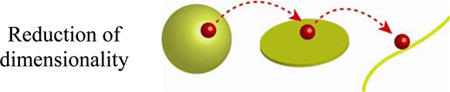 |
|
Speeds up targeting or increases depth of penetration into cell | |
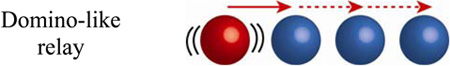 |
|
Accelerates signal transduction, amplifies signals | |
 |
|
Extends the “reach” of complexed chemicals | |
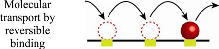 |
|
|
Crosslinks and strengthens filopodia |
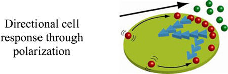 |
|
Protrusion and directed motility along chemoattractant gradients | |
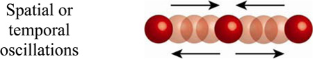 |
|
Precise positioning of cellular structures; Frequency-specific responses | |
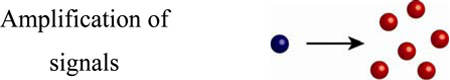 |
|
Sensing of chemoattractants | |
 |
|
Toggling between different functional states |
We close with some general observations we made while writing the manuscript. The first one is that diffusion is not at all a boring subject typically associated with “smearing-up” concentration gradients and with wasteful dissipation of chemical energy. When properly synchronized with chemical reactions, it can become a purposeful and powerful tool with which to transport, position, and control small-scale structures. In doing so, it can be amazingly precise – take, for instance, the Min system, where RD places the Z-ring with precision of ~1% of the cell’s length (tens of nanometers!). The second, and related point is that we are only beginning to learn about the astounding prowess and richness of cellular phenomena stemming from RD. While the macroscopic RD systems such as Turing or BZ patterns have been studied for decades, many papers on cellular RD we have cited in this Review are quite recent suggesting that this area of study is taking off. As the resolution of in-cell microscopy techniques[12–17, 266] improves, one might expect that more and more experimentalists will be able to track the paths of molecules within cells and more RD processes are likely to be discovered. It should be pointed out, however, that for this study to become science rather than (Lord Rutherford’s) “stamp-collecting”,[267] experiments must go hand-in hand with theory. Reaction-diffusion is simply too complex and often counter intuitive to understand without mathematical models. Fortunately, the construction and solution of RD equations follows well-defined rules, some of which we hope to have expounded in the present paper; more information on the mathematics of RD can be found in recent monographs on the subject.[64, 71, 268] Overall, further journey into the realm of cellular RD might not necessarily be easy and might require a combination of tools from various disciplines (chemistry, cell biology, imaging, mathematics, physics), but it certainly promises to be a great adventure.
Supplementary Material
Acknowledgements
This work was supported by grant #1U54CA119341-01, awarded by National Institutes of Health/ National Cancer Institute (NIH/NCI) and by the Center of Cancer Nanotechnology Excellence (CCNE) at Northwestern University, NIH grant #1R21CA137707-01 (both to BAG).
Biographies

Siowling Soh graduated with First Class Honors in chemical engineering from the National University of Singapore in 2002. He is currently a PhD candidate working with Prof. Bartosz A. Grzybowski in the Departments of Chemistry and of Chemical and Biological Engineering at Northwestern University. His scientific interests focus on complex chemical systems with emphasis on reaction-diffusion and reaction networks.

Marta Byrska received her M.Sc. degree in Biology from Jagiellonian University (Krakow, Poland) in 2007 with research conducted at the University of Chicago in the Department of Biochemistry and Molecular Biology. She is currently a graduate student with Prof. Bartosz A. Grzybowski at Northwestern University. Her research focuses on cell motility at the molecular level, in particular on the synchronization of actin filaments, microtubules and focal adhesions during migration of cancerous cells.

Kristiana Kandere-Grzybowska graduated summa cum laude in biology from the College of Saint Rose in 1998. She obtained doctoral degree in biochemistry from Tufts University in September 2003 (with T.C. Theoharides) followed by Department of Defense postdoctoral fellowship at Northwestern University. She is currently Research Assistant Professor working together with Prof. Bartosz A. Grzybowski in the Departments of Chemistry and of Chemical and Biological Engineering at Northwestern University. Her research interests are intracellular/cytoskeleton dynamics and cell motility in defined geometric confines and in cancer.

Bartosz A. Grzybowski graduated summa cum laude and Honoris in Chimia from Yale University in 1995. He obtained his doctoral degree in physical chemistry from Harvard University in August 2000 (with G. M. Whitesides). In June 2003, he joined the Faculty of Northwestern University where he is now Burgess Professor of Physical Chemistry and Chemical Systems Engineering. His scientific interests include self-assembly in non-equilibrium/dynamic systems, complex chemical networks, nanostructured materials and nanobiology. Prof. Grzybowski is a recipient of the ACS Colloids Young Investigator, NSF CAREER, and Gerhard Kanig Innovation Awards, and has recently been named a Pew Scholar in Biomedical Sciences, a Sloan Fellow and a Dreyfus Teacher-Scholar. His first book “Chemistry in Motion: Reaction-Diffusion Systems in Micro- and Nanotechnology” from Wiley was published earlier this year.
Contributor Information
Siowling Soh, Department of Chemical and Biological Engineering, Northwestern University, 2145 Sheridan Rd, Evanston, IL 60208.
Marta Byrska, Department of Chemical and Biological Engineering, Northwestern University, 2145 Sheridan Rd, Evanston, IL 60208.
Kristiana Kandere-Grzybowska, Department of Chemical and Biological Engineering, Northwestern University, 2145 Sheridan Rd, Evanston, IL 60208.
Bartosz A. Grzybowski, Department of Chemistry, Department of Chemical and Biological Engineering, Northwestern University, 2145 Sheridan Rd, Evanston, IL 60208, grzybor@northwestern.edu Homepage: http://www.dysa.northwestern.edu
References and Notes
- 1.Kholodenko BN, Kolch W. Cell. 2008;133:566. doi: 10.1016/j.cell.2008.04.033. [DOI] [PubMed] [Google Scholar]
- 2.Shimomura O, Johnson FH, Saiga Y. J. Cell. Comp. Physiol. 1962;59:223. doi: 10.1002/jcp.1030590302. [DOI] [PubMed] [Google Scholar]
- 3.Chalfie M, Tu Y, Euskirchen G, Ward WW, Prasher DC. Science. 1994;263:802. doi: 10.1126/science.8303295. [DOI] [PubMed] [Google Scholar]
- 4.Heim R, Prasher DC, Tsien RY. Proc. Natl. Acad. Sci. U. S. A. 1994;91:12501. doi: 10.1073/pnas.91.26.12501. [DOI] [PMC free article] [PubMed] [Google Scholar]
- 5.Shimomura O. Angew. Chem. 2009;121:5698. [Google Scholar]; Angew. Chem. Int. Ed. 2009;48:5590. [Google Scholar]
- 6.Chalfie M. Angew. Chem. 2009;121:5711. [Google Scholar]; Angew. Chem. Int. Ed. 2009;48:5603. [Google Scholar]
- 7.Tsien RY. Angew. Chem. 2009;121:5721. [Google Scholar]; Angew. Chem. Int. Ed. 2009;48:5612. [Google Scholar]
- 8.Jares-Erijman EA, Jovin TM. Nat. Biotechnol. 2003;21:1387. doi: 10.1038/nbt896. [DOI] [PubMed] [Google Scholar]
- 9.Atkins P, de Paula J. Physical Chemistry. 7th ed. New York: W. H. Freeman and Company; 2001. [Google Scholar]
- 10.Levine I. Physical Chemistry. 6th ed. New York: McGraw-Hill; 2008. [Google Scholar]
- 11.McQuarrie DA, Simon JD. Physical Chemistry: A Molecular Approach. University Science Books, Sausalito; 1997. [Google Scholar]
- 12.Huang B, Wang WQ, Bates M, Zhuang XW. Science. 2008;319:810. doi: 10.1126/science.1153529. [DOI] [PMC free article] [PubMed] [Google Scholar]
- 13.Rust MJ, Bates M, Zhuang XW. Nat. Methods. 2006;3:793. doi: 10.1038/nmeth929. [DOI] [PMC free article] [PubMed] [Google Scholar]
- 14.Hell SW. Nat. Biotechnol. 2003;21:1347. doi: 10.1038/nbt895. [DOI] [PubMed] [Google Scholar]
- 15.Hell SW. Science. 2007;316:1153. doi: 10.1126/science.1137395. [DOI] [PubMed] [Google Scholar]
- 16.Betzig E, Patterson GH, Sougrat R, Lindwasser OW, Olenych S, Bonifacino JS, Davidson MW, Lippincott-Schwartz J, Hess HF. Science. 2006;313:1642. doi: 10.1126/science.1127344. [DOI] [PubMed] [Google Scholar]
- 17.Gustafsson MGL. Proc. Natl. Acad. Sci. U. S. A. 2005;102:13081. doi: 10.1073/pnas.0406877102. [DOI] [PMC free article] [PubMed] [Google Scholar]
- 18.Durr NJ, Larson T, Smith DK, Korgel BA, Sokolov K, Ben-Yakar A. Nano Lett. 2007;7:941. doi: 10.1021/nl062962v. [DOI] [PMC free article] [PubMed] [Google Scholar]
- 19.Sonnichsen C, Alivisatos AP. Nano Lett. 2005;5:301. doi: 10.1021/nl048089k. [DOI] [PubMed] [Google Scholar]
- 20.Wang HF, Huff TB, Zweifel DA, He W, Low PS, Wei A, Cheng JX. Proc. Natl. Acad. Sci. U. S. A. 2005;102:15752. doi: 10.1073/pnas.0504892102. [DOI] [PMC free article] [PubMed] [Google Scholar]
- 21.Chen J, et al. Nano Lett. 2005;5:473. doi: 10.1021/nl047950t. [DOI] [PubMed] [Google Scholar]
- 22.Chen JY, et al. Adv. Mater. 2005;17:2255. [Google Scholar]
- 23.Kircher MF, Mahmood U, King RS, Weissleder R, Josephson L. Cancer Res. 2003;63:8122. [PubMed] [Google Scholar]
- 24.Bulte JWM, Kraitchman DL. NMR Biomed. 2004;17:484. doi: 10.1002/nbm.924. [DOI] [PubMed] [Google Scholar]
- 25.Zhao M, Beauregard DA, Loizou L, Davletov B, Brindle KM. Nat. Med. 2001;7:1241. doi: 10.1038/nm1101-1241. [DOI] [PubMed] [Google Scholar]
- 26.Chan WCW, Maxwell DJ, Gao XH, Bailey RE, Han MY, Nie SM. Curr. Opin. Biotechnol. 2002;13:40. doi: 10.1016/s0958-1669(02)00282-3. [DOI] [PubMed] [Google Scholar]
- 27.Mitchell P. Nat. Biotechnol. 2001;19:1013. doi: 10.1038/nbt1101-1013. [DOI] [PubMed] [Google Scholar]
- 28.Klarreich E. Nature. 2001;413:450. doi: 10.1038/35097256. [DOI] [PubMed] [Google Scholar]
- 29.Ludlow RF, Otto S. Chem. Soc. Rev. 2008;37:101. doi: 10.1039/b611921m. [DOI] [PubMed] [Google Scholar]
- 30.Wagner N, Ashkenasy G. Chem.-Eur. J. 2009;15:1765. doi: 10.1002/chem.200801850. [DOI] [PubMed] [Google Scholar]
- 31.Dadon Z, Wagner N, Ashkenasy G. Angew. Chem. 2008;120:6221. doi: 10.1002/anie.200702552. [DOI] [PubMed] [Google Scholar]; Angew. Chem. Int. Ed. 2008;47:6128. [Google Scholar]
- 32.Hjelmfelt A, Weinberger ED, Ross J. Proc. Natl. Acad. Sci. U. S. A. 1991;88:10983. doi: 10.1073/pnas.88.24.10983. [DOI] [PMC free article] [PubMed] [Google Scholar]
- 33.Arkin A, Ross J. Biophys. J. 1994;67:560. doi: 10.1016/S0006-3495(94)80516-8. [DOI] [PMC free article] [PubMed] [Google Scholar]
- 34.Lodish H, Berk A, Matsudaira P, Kaiser CA, Krieger M, Scott MP, Zipursky SL, Darnell J. Molecular Cell Biology. 5th ed. New York: W.H. Freeman and Company; 2004. [Google Scholar]
- 35.Murray JD. Mathematical Biology: An Introduction. 3rd ed. Vol. 1. New York: Springer-Verlag; 2002. [Google Scholar]
- 36.Murray JD. Mathematical Biology: Spatial Models and Biomedical Applications. 3rd ed. Vol. 2. New York: Springer-Verlag; 2003. [Google Scholar]
- 37.Zaikin AN, Zhabotinsky AM. Nature. 1970;225:535. doi: 10.1038/225535b0. [DOI] [PubMed] [Google Scholar]
- 38.Field RJ, Burger M. Oscillations and traveling waves in chemical systems. New York: John Wiley & Sons; 1985. [Google Scholar]
- 39.Bishop KJM, Grzybowski BA. Phys. Rev. Lett. 2006;97:128702. doi: 10.1103/PhysRevLett.97.128702. [DOI] [PubMed] [Google Scholar]
- 40.Wood PM, Ross J. J. Chem. Phys. 1985;82:1924. [Google Scholar]
- 41.Hanna A, Saul A, Showalter K. J. Am. Chem. Soc. 1982;104:3838. [Google Scholar]
- 42.Dekepper P, Epstein IR, Kustin K, Orban M. J. Phys. Chem. 1982;86:170. [Google Scholar]
- 43.Ross J, Muller SC, Vidal C. Science. 1988;240:460. doi: 10.1126/science.240.4851.460. [DOI] [PubMed] [Google Scholar]
- 44.Vanag VK, Yang LF, Dolnik M, Zhabotinsky AM, Epstein IR. Nature. 2000;406:389. doi: 10.1038/35019038. [DOI] [PubMed] [Google Scholar]
- 45.Lee KJ, McCormick WD, Ouyang Q, Swinney HL. Science. 1993;261:192. doi: 10.1126/science.261.5118.192. [DOI] [PubMed] [Google Scholar]
- 46.Ertl G. Science. 1991;254:1750. doi: 10.1126/science.254.5039.1750. [DOI] [PubMed] [Google Scholar]
- 47.Wolff J, Papathanasiou AG, Kevrekidis IG, Rotermund HH, Ertl G. Science. 2001;294:134. doi: 10.1126/science.1063597. [DOI] [PubMed] [Google Scholar]
- 48.Liesegang RE. Naturwiss. Wochenschr. 1896;10:353. [Google Scholar]
- 49.Chopard B, Luthi P, Droz M. Phys. Rev. Lett. 1994;72:1384. doi: 10.1103/PhysRevLett.72.1384. [DOI] [PubMed] [Google Scholar]
- 50.Fialkowski M, Bitner A, Grzybowski BA. Phys. Rev. Lett. 2005;94:018303. doi: 10.1103/PhysRevLett.94.018303. [DOI] [PubMed] [Google Scholar]
- 51.Flicker M, Ross J. J. Chem. Phys. 1974;60:3458. [Google Scholar]
- 52.Muller SC, Ross J. J. Phys. Chem. A. 2003;107:7997. [Google Scholar]
- 53.Ammelt E, Schweng D, Purwins HG. Phys. Lett. A. 1993;179:348. [Google Scholar]
- 54.Gurevich EL, Zanin AL, Moskalenko AS, Purwins HG. Phys. Rev. Lett. 2003;91:154501. doi: 10.1103/PhysRevLett.91.154501. [DOI] [PubMed] [Google Scholar]
- 55.Heaney PJ, Davis AM. Science. 1995;269:1562. doi: 10.1126/science.269.5230.1562. [DOI] [PubMed] [Google Scholar]
- 56.Short MB, Baygents JC, Beck JW, Stone DA, Toomey RS, Goldstein RE. Phys. Rev. Lett. 2005;94:018501. doi: 10.1103/PhysRevLett.94.018501. [DOI] [PubMed] [Google Scholar]
- 57.Glossary of Geology. 3rd ed. Alexandria: American Geological Institute; 1987. [Google Scholar]
- 58.Budrene EO, Berg HC. Nature. 1991;349:630. doi: 10.1038/349630a0. [DOI] [PubMed] [Google Scholar]
- 59.Budrene EO, Berg HC. Nature. 1995;376:49. doi: 10.1038/376049a0. [DOI] [PubMed] [Google Scholar]
- 60.Hess B. Naturwissenschaften. 2000;87:199. doi: 10.1007/s001140050704. [DOI] [PubMed] [Google Scholar]
- 61.Winfree AT. The Geometry of Biological Time. 2nd ed. New York: Springer-Verlag; 2001. [Google Scholar]
- 62.Kondo S, Asai R. Nature. 1995;376:765. doi: 10.1038/376765a0. [DOI] [PubMed] [Google Scholar]
- 63.Jiang TX, Widelitz RB, Shen WM, Will P, Wu DY, Lin CM, Jung HS, Chuong CM. Int. J. Dev. Biol. 2004;48:117. doi: 10.1387/ijdb.041788tj. [DOI] [PMC free article] [PubMed] [Google Scholar]
- 64.Deen WM. Analysis of Transport Phenomena. New York: Oxford University Press; 1998. [Google Scholar]
- 65.Van Kampen NG. Stochastic Processes in Physics and Chemistry. New York: Elsevier Science Publishers; 1981. [Google Scholar]
- 66.Metzler R, Klafter J. Phys. Rep.-Rev. Sec. Phys. Lett. 2000;339:1. [Google Scholar]
- 67.Turing AM. Philos. Trans. R. Soc. Lond. 1952;237:37. [Google Scholar]
- 68.Miura T, Matsumoto T. Proc. R. Soc. Lond. 2000;267:1185. doi: 10.1098/rspb.2000.1127. [DOI] [PMC free article] [PubMed] [Google Scholar]
- 69.Miura T. Insect. Soc. 2001;48:216. [Google Scholar]
- 70.Siegert F, Weijer CJ. Curr. Biol. 1995;5:937. doi: 10.1016/s0960-9822(95)00184-9. [DOI] [PubMed] [Google Scholar]
- 71.Grzybowski BA. Chemistry in Motion: Reaction-Diffusion Systems for Micro- and Nanotechnology. Chichester, UK: John Wiley & Sons; 2009. [Google Scholar]
- 72.Elowitz MB, Surette MG, Wolf PE, Stock JB, Leibler S. J. Bacteriol. 1999;181:197. doi: 10.1128/jb.181.1.197-203.1999. [DOI] [PMC free article] [PubMed] [Google Scholar]
- 73.Swaminathan R, Hoang CP, Verkman AS. Biophys. J. 1997;72:1900. doi: 10.1016/S0006-3495(97)78835-0. [DOI] [PMC free article] [PubMed] [Google Scholar]
- 74.Meyers J, Craig J, Odde DJ. Curr. Biol. 2006;16:1685. doi: 10.1016/j.cub.2006.07.056. [DOI] [PubMed] [Google Scholar]
- 75.Alberts B, Johnson A, Lewis J, Raff M, Roberts K, Walter P. Molecular Biology of the Cell. 4th ed. New York: Garland Science; 2002. [Google Scholar]
- 76.Howard J. Annu. Rev. Physiol. 1996;58:703. doi: 10.1146/annurev.ph.58.030196.003415. [DOI] [PubMed] [Google Scholar]
- 77.Lee JS, Mayes MS, Stromer MH, Scanes CG, Jeftinija S, Anderson LL. Exp. Biol. Med. 2004;229:632. doi: 10.1177/153537020422900707. [DOI] [PubMed] [Google Scholar]
- 78.Wacker I, Kaether C, Kromer A, Migala A, Almers W, Gerdes HH. J. Cell Sci. 1997;110:1453. doi: 10.1242/jcs.110.13.1453. [DOI] [PubMed] [Google Scholar]
- 79.Culic O, Gruwel MLH, Schrader J. Am. J. Physiol. 1997;273:C205. doi: 10.1152/ajpcell.1997.273.1.C205. [DOI] [PubMed] [Google Scholar]
- 80.Ghaemmaghami S, Huh W, Bower K, Howson RW, Belle A, Dephoure N, O'Shea EK, Weissman JS. Nature. 2003;425:737. doi: 10.1038/nature02046. [DOI] [PubMed] [Google Scholar]
- 81.Giannakakou P, Sackett DL, Ward Y, Webster KR, Blagosklonny MV, Fojo T. Nat. Cell Biol. 2000;2:709. doi: 10.1038/35036335. [DOI] [PubMed] [Google Scholar]
- 82.Prahlad V, Helfand BT, Langford GM, Vale RD, Goldman RD. J. Cell Sci. 2000;113:3939. doi: 10.1242/jcs.113.22.3939. [DOI] [PubMed] [Google Scholar]
- 83.Mimori-Kiyosue Y, Shiina N, Tsukita S. J. Cell Biol. 2000;148:505. doi: 10.1083/jcb.148.3.505. [DOI] [PMC free article] [PubMed] [Google Scholar]
- 84.Trostel SY, Sackett DL, Fojo T. Cell Cycle. 2006;5:2253. doi: 10.4161/cc.5.19.3291. [DOI] [PubMed] [Google Scholar]
- 85.Garner EC, Campbell CS, Mullins RD. Science. 2004;306:1021. doi: 10.1126/science.1101313. [DOI] [PubMed] [Google Scholar]
- 86.Garner EC, Campbell CS, Weibel DB, Mullins RD. Science. 2007;315:1270. doi: 10.1126/science.1138527. [DOI] [PMC free article] [PubMed] [Google Scholar]
- 87.Popp D, Yamamoto A, Iwasa M, Narita A, Maeda K, Maeda Y. Biochem. Biophys. Res. Commun. 2007;353:109. doi: 10.1016/j.bbrc.2006.11.130. [DOI] [PubMed] [Google Scholar]
- 88.Moller-Jensen J, Borch J, Dam M, Jensen RB, Roepstorff P, Gerdes K. Mol. Cell. 2003;12:1477. doi: 10.1016/s1097-2765(03)00451-9. [DOI] [PubMed] [Google Scholar]
- 89.Fogel MA, Waldor MK. Genes Dev. 2006;20:3269. doi: 10.1101/gad.1496506. [DOI] [PMC free article] [PubMed] [Google Scholar]
- 90.Moller-Jensen J, Jensen RB, Gerdes K. Trends Microbiol. 2000;8:313. doi: 10.1016/s0966-842x(00)01787-x. [DOI] [PubMed] [Google Scholar]
- 91.Mohl DA, Gober JW. Cell. 1997;88:675. doi: 10.1016/s0092-8674(00)81910-8. [DOI] [PubMed] [Google Scholar]
- 92.Gerdes K, Moller-Jensen J, Jensen RB. Mol. Microbiol. 2000;37:455. doi: 10.1046/j.1365-2958.2000.01975.x. [DOI] [PubMed] [Google Scholar]
- 93.Stock AM, Robinson VL, Goudreau PN. Annu. Rev. Biochem. 2000;69:183. doi: 10.1146/annurev.biochem.69.1.183. [DOI] [PubMed] [Google Scholar]
- 94.Hoch JA. Curr. Opin. Microbiol. 2000;3:165. doi: 10.1016/s1369-5274(00)00070-9. [DOI] [PubMed] [Google Scholar]
- 95.Wadhams GH, Armitage JP. Nat. Rev. Mol. Cell Biol. 2004;5:1024. doi: 10.1038/nrm1524. [DOI] [PubMed] [Google Scholar]
- 96.Maddock JR, Shapiro L. Science. 1993;259:1717. doi: 10.1126/science.8456299. [DOI] [PubMed] [Google Scholar]
- 97.Khan S, Spudich JL, McCray JA, Trentham DR. Proc. Natl. Acad. Sci. U. S. A. 1995;92:9757. doi: 10.1073/pnas.92.21.9757. [DOI] [PMC free article] [PubMed] [Google Scholar]
- 98.Segall JE, Manson MD, Berg HC. Nature. 1982;296:855. doi: 10.1038/296855a0. [DOI] [PubMed] [Google Scholar]
- 99.Segall JE, Ishihara A, Berg HC. J. Bacteriol. 1985;161:51. doi: 10.1128/jb.161.1.51-59.1985. [DOI] [PMC free article] [PubMed] [Google Scholar]
- 100.Camacho CJ, Kimura SR, DeLisi C, Vajda S. Biophys. J. 2000;78:1094. doi: 10.1016/S0006-3495(00)76668-9. [DOI] [PMC free article] [PubMed] [Google Scholar]
- 101.Duke TAJ, Le Novere N, Bray D. J. Mol. Biol. 2001;308:541. doi: 10.1006/jmbi.2001.4610. [DOI] [PubMed] [Google Scholar]
- 102.Cluzel P, Surette M, Leibler S. Science. 2000;287:1652. doi: 10.1126/science.287.5458.1652. [DOI] [PubMed] [Google Scholar]
- 103.Lipkow K, Andrews SS, Bray D. J. Bacteriol. 2005;187:45. doi: 10.1128/JB.187.1.45-53.2005. [DOI] [PMC free article] [PubMed] [Google Scholar]
- 104.Alon U, Surette MG, Barkai N, Leibler S. Nature. 1999;397:168. doi: 10.1038/16483. [DOI] [PubMed] [Google Scholar]
- 105.Almogy G, Stone L, Ben-Tal N. Biophys. J. 2001;81:3016. doi: 10.1016/S0006-3495(01)75942-5. [DOI] [PMC free article] [PubMed] [Google Scholar]
- 106.Vaknin A, Berg HC. Proc. Natl. Acad. Sci. U. S. A. 2004;101:17072. doi: 10.1073/pnas.0407812101. [DOI] [PMC free article] [PubMed] [Google Scholar]
- 107.Bi E, Lutkenhaus J. Nature. 1991;354:161. doi: 10.1038/354161a0. [DOI] [PubMed] [Google Scholar]
- 108.Trueba FJ. Arch. Microbiol. 1982;131:55. doi: 10.1007/BF00451499. [DOI] [PubMed] [Google Scholar]
- 109.Howard M, Rutenberg AD, de Vet S. Phys. Rev. Lett. 2001;87:278102. doi: 10.1103/PhysRevLett.87.278102. [DOI] [PubMed] [Google Scholar]
- 110.Meinhardt H, de Boer PAJ. Proc. Natl. Acad. Sci. U. S. A. 2001;98:14202. doi: 10.1073/pnas.251216598. [DOI] [PMC free article] [PubMed] [Google Scholar]
- 111.Kruse K. Biophys. J. 2002;82:618. doi: 10.1016/S0006-3495(02)75426-X. [DOI] [PMC free article] [PubMed] [Google Scholar]
- 112.Howard M, Rutenberg AD. Phys. Rev. Lett. 2003;90:128102. doi: 10.1103/PhysRevLett.90.128102. [DOI] [PubMed] [Google Scholar]
- 113.Huang KC, Meir Y, Wingreen NS. Proc. Natl. Acad. Sci. U. S. A. 2003;100:12724. doi: 10.1073/pnas.2135445100. [DOI] [PMC free article] [PubMed] [Google Scholar]
- 114.Kulkarni RV, Huang KC, Kloster M, Wingreen NS. Phys. Rev. Lett. 2004;93:228103. doi: 10.1103/PhysRevLett.93.228103. [DOI] [PubMed] [Google Scholar]
- 115.Raskin DM, de Boer PAJ. Proc. Natl. Acad. Sci. U. S. A. 1999;96:4971. doi: 10.1073/pnas.96.9.4971. [DOI] [PMC free article] [PubMed] [Google Scholar]
- 116.Zhou H, Lutkenhaus J. J. Bacteriol. 2003;185:4326. doi: 10.1128/JB.185.15.4326-4335.2003. [DOI] [PMC free article] [PubMed] [Google Scholar]
- 117.Lutkenhaus J. Annu. Rev. Biochem. 2007;76:539. doi: 10.1146/annurev.biochem.75.103004.142652. [DOI] [PubMed] [Google Scholar]
- 118.Romberg L, Levin PA. Annu. Rev. Microbiol. 2003;57:125. doi: 10.1146/annurev.micro.57.012903.074300. [DOI] [PMC free article] [PubMed] [Google Scholar]
- 119.Hu T, Shklovskii BI. Phys. Rev. E. 2006;74:021903. doi: 10.1103/PhysRevE.74.021903. [DOI] [PubMed] [Google Scholar]
- 120.Ptashne M, Gann A. Essays Biochem. 2001;37:1. doi: 10.1042/bse0370001. [DOI] [PubMed] [Google Scholar]
- 121.Klenin KV, Merlitz H, Langowski J, Wu CX. Phys. Rev. Lett. 2006;96:018104. doi: 10.1103/PhysRevLett.96.018104. [DOI] [PubMed] [Google Scholar]
- 122.von Hippel PH. Annu. Rev. Biophys. Biomol. Struct. 2007;36:79. doi: 10.1146/annurev.biophys.34.040204.144521. [DOI] [PMC free article] [PubMed] [Google Scholar]
- 123.Widom J. Proc. Natl. Acad. Sci. U. S. A. 2005;102:16909. doi: 10.1073/pnas.0508686102. [DOI] [PMC free article] [PubMed] [Google Scholar]
- 124.Riggs AD, Bourgeoi S, Cohn M. J. Mol. Biol. 1970;53:401. doi: 10.1016/0022-2836(70)90074-4. [DOI] [PubMed] [Google Scholar]
- 125.Halford SE, Marko JF. Nucleic Acids Res. 2004;32:3040. doi: 10.1093/nar/gkh624. [DOI] [PMC free article] [PubMed] [Google Scholar]
- 126.Wang YM, Austin RH, Cox EC. Phys. Rev. Lett. 2006;97:048302. doi: 10.1103/PhysRevLett.97.048302. [DOI] [PubMed] [Google Scholar]
- 127.Gowers DM, Wilson GG, Halford SE. Proc. Natl. Acad. Sci. U. S. A. 2005;102:15883. doi: 10.1073/pnas.0505378102. [DOI] [PMC free article] [PubMed] [Google Scholar]
- 128.van den Broek B, Lomholt MA, Kalisch SMJ, Metzler R, Wuite GJL. Proc. Natl. Acad. Sci. U. S. A. 2008;105:15738. doi: 10.1073/pnas.0804248105. [DOI] [PMC free article] [PubMed] [Google Scholar]
- 129.Bustamante C, Guthold M, Zhu XS, Yang GL. J. Biol. Chem. 1999;274:16665. doi: 10.1074/jbc.274.24.16665. [DOI] [PubMed] [Google Scholar]
- 130.Shimamoto N. J. Biol. Chem. 1999;274:15293. doi: 10.1074/jbc.274.22.15293. [DOI] [PubMed] [Google Scholar]
- 131.Givaty O, Levy Y. J. Mol. Biol. 2009;385:1087. doi: 10.1016/j.jmb.2008.11.016. [DOI] [PubMed] [Google Scholar]
- 132.An interesting variant of the jumping mechanism is observed in proteins having more than one DNA binding domains ( Halford SE, Gowers DM, Sessions RB. Nat. Struct. Biol. 2000;7:705. doi: 10.1038/78911. ) – for example, the V-shaped lac repressor, whose both “tips” can bind to DNA and can thus bring together two distant DNA loci. When this happens, thermal fluctuations can mediate the so-called intersegmental transfer of the protein from one DNA segment to another ( Berg OG, Winter RB, von Hippel PH. Biochemistry. 1981;20:6929. doi: 10.1021/bi00527a028. ). Similar to “jumping”, this mechanism allows the protein to travel hundreds of base pair away from its current site. However, while “jumping” involves dissociation of the protein from the DNA, the protein remains bound to the DNA during intersegmental transfer. Intersegmental transfer has been observed directly through scanning force microscopy (SFM) for E. coli RNA Polymerase on DNA ( Bustamante C, Guthold M, Zhu X, Yang G. J. Biol. Chem. 1999;274:16665. doi: 10.1074/jbc.274.24.16665. ) and has also been implicated to occur in the lac repressor ( Fried MG, Crothers DM. J. Mol. Biol. 1984;172:263. doi: 10.1016/s0022-2836(84)80026-1.).
- 133.Porecha RH, Stivers JT. Proc. Natl. Acad. Sci. U. S. A. 2008;105:10791. doi: 10.1073/pnas.0801612105. [DOI] [PMC free article] [PubMed] [Google Scholar]
- 134.Berg OG, Winter RB, Von Hippel PH. Biochemistry. 1981;20:6929. doi: 10.1021/bi00527a028. [DOI] [PubMed] [Google Scholar]
- 135.Viswanathan GM, Buldyrev SV, Havlin S, da Luz MGE, Raposo EP, Stanley HE. Nature. 1999;401:911. doi: 10.1038/44831. [DOI] [PubMed] [Google Scholar]
- 136.Bartumeus F, Da Luz MGE, Viswanathan GM, Catalan J. Ecology. 2005;86:3078. [Google Scholar]
- 137.Viswanathan GM, Afanasyev V, Buldyrev SV, Murphy EJ, Prince PA, Stanley HE. Nature. 1996;381:413. [Google Scholar]
- 138.Bartumeus F, Peters F, Pueyo S, Marrase C, Catalan J. Proc. Natl. Acad. Sci. U. S. A. 2003;100:12771. doi: 10.1073/pnas.2137243100. [DOI] [PMC free article] [PubMed] [Google Scholar]
- 139.Lomholt MA, Ambjornsson T, Metzler R. Phys. Rev. Lett. 2005;95:260603. doi: 10.1103/PhysRevLett.95.260603. [DOI] [PubMed] [Google Scholar]
- 140.Barkley MD. Biochemistry. 1981;20:3833. doi: 10.1021/bi00516a026. [DOI] [PubMed] [Google Scholar]
- 141.Lang BF, Gray MW, Burger G. Annu. Rev. Genet. 1999;33:351. doi: 10.1146/annurev.genet.33.1.351. [DOI] [PubMed] [Google Scholar]
- 142.Martin W, Stoebe B, Goremykin V, Hansmann S, Hasegawa M, Kowallik KV. Nature. 1998;393:162. doi: 10.1038/30234. [DOI] [PubMed] [Google Scholar]
- 143.Margulis L, Stolz JF. Adv. Space Res. 1984;4:195. doi: 10.1016/0273-1177(84)90562-3. [DOI] [PubMed] [Google Scholar]
- 144.de Duve C. Sci. Am. 1996;274:50. doi: 10.1038/scientificamerican0496-50. [DOI] [PubMed] [Google Scholar]
- 145.de Duve C. Nat. Rev. Genet. 2007;8:395. doi: 10.1038/nrg2071. [DOI] [PubMed] [Google Scholar]
- 146.Schott DH, Collins RN, Bretscher A. J. Cell Biol. 2002;156:35. doi: 10.1083/jcb.200110086. [DOI] [PMC free article] [PubMed] [Google Scholar]
- 147.Mohr E. Prog. Neurobiol. 1999;57:507. doi: 10.1016/s0301-0082(98)00066-5. [DOI] [PubMed] [Google Scholar]
- 148.Bashirullah A, Cooperstock RL, Lipshitz HD. Annu. Rev. Biochem. 1998;67:335. doi: 10.1146/annurev.biochem.67.1.335. [DOI] [PubMed] [Google Scholar]
- 149.Lasko P. FASEB J. 1999;13:421. doi: 10.1096/fasebj.13.3.421. [DOI] [PubMed] [Google Scholar]
- 150.Mowry KL, Cote CA. FASEB J. 1999;13:435. doi: 10.1096/fasebj.13.3.435. [DOI] [PubMed] [Google Scholar]
- 151.Bassell GJ, Oleynikov Y, Singer RH. FASEB J. 1999;13:447. doi: 10.1096/fasebj.13.3.447. [DOI] [PubMed] [Google Scholar]
- 152.Carson JH, Kwon SJ, Barbarese E. Curr. Opin. Neurobiol. 1998;8:607. doi: 10.1016/s0959-4388(98)80088-3. [DOI] [PubMed] [Google Scholar]
- 153.Deshler JO, Highett MI, Abramson T, Schnapp BJ. Curr. Biol. 1998;8:489. doi: 10.1016/s0960-9822(98)70200-3. [DOI] [PubMed] [Google Scholar]
- 154.King ML, Zhou Y, Bubunenko M. Bioessays. 1999;21:546. doi: 10.1002/(SICI)1521-1878(199907)21:7<546::AID-BIES3>3.0.CO;2-Z. [DOI] [PubMed] [Google Scholar]
- 155.Steward O. Neuron. 1997;18:9. doi: 10.1016/s0896-6273(01)80041-6. [DOI] [PubMed] [Google Scholar]
- 156.Takizawa PA, Sil A, Swedlow JR, Herskowitz I, Vale RD. Nature. 1997;389:90. doi: 10.1038/38015. [DOI] [PubMed] [Google Scholar]
- 157.Another motif commonly found in signaling pathways is composed of two forms of protein: active one - bound to GTP, and inactive one - bound to GDP nucleotide. This convertible system is controlled by two types of proteins of "opposing" activities – GEF (guanine exchange factor) that catalyses the GDP to GTP exchange, and GAP (GTPase activating protein) that induces the hydrolysis of GTP to GDP.
- 158.Yudushkin IA, Schleifenbaum A, Kinkhabwala A, Neel BG, Schultz C, Bastiaens PIH. Science. 2007;315:115. doi: 10.1126/science.1134966. [DOI] [PubMed] [Google Scholar]
- 159.Brown GC, Kholodenko BN. FEBS Lett. 1999;457:452. doi: 10.1016/s0014-5793(99)01058-3. [DOI] [PubMed] [Google Scholar]
- 160.Bastiaens P, Caudron M, Niethammer P, Karsenti E. Trends Cell Biol. 2006;16:125. doi: 10.1016/j.tcb.2006.01.005. [DOI] [PubMed] [Google Scholar]
- 161.Kholodenko BN. Trends Cell Biol. 2002;12:173. doi: 10.1016/s0962-8924(02)02251-1. [DOI] [PubMed] [Google Scholar]
- 162.Kholodenko BN. Nat. Rev. Mol. Cell Biol. 2006;7:165. doi: 10.1038/nrm1838. [DOI] [PMC free article] [PubMed] [Google Scholar]
- 163.Markevich NI, Tsyganov MA, Hoek JB, Kholodenko BN. Mol. Syst. Biol. 2006;2:8. doi: 10.1038/msb4100108. [DOI] [PMC free article] [PubMed] [Google Scholar]
- 164.Tischer C, Bastiaens PIH. Nat. Rev. Mol. Cell Biol. 2003;4:971. doi: 10.1038/nrm1258. [DOI] [PubMed] [Google Scholar]
- 165.Hubbard SR, Mohammadi M, Schlessinger J. J. Biol. Chem. 1998;273:11987. doi: 10.1074/jbc.273.20.11987. [DOI] [PubMed] [Google Scholar]
- 166.Verveer PJ, Wouters FS, Reynolds AR, Bastiaens PIH. Science. 2000;290:1567. doi: 10.1126/science.290.5496.1567. [DOI] [PubMed] [Google Scholar]
- 167.Carpenter G, Lembach KJ, Morrison MM, Cohen S. J. Biol. Chem. 1975;250:4297. [PubMed] [Google Scholar]
- 168.Cuvelier D, Thery M, Chu YS, Dufour S, Thiery JP, Bornens M, Nassoy P, Mahadevan L. Curr. Biol. 2007;17:694. doi: 10.1016/j.cub.2007.02.058. [DOI] [PubMed] [Google Scholar]
- 169.Lechleiter J, Girard S, Peralta E, Clapham D. Science. 1991;252:123. doi: 10.1126/science.2011747. [DOI] [PubMed] [Google Scholar]
- 170.Berridge MJ. Nature. 1993;361:315. doi: 10.1038/361315a0. [DOI] [PubMed] [Google Scholar]
- 171.Berridge MJ. J. Exp. Biol. 1997;200:315. doi: 10.1242/jeb.200.2.315. [DOI] [PubMed] [Google Scholar]
- 172.Stricker SA. Dev. Biol. 1995;170:496. doi: 10.1006/dbio.1995.1232. [DOI] [PubMed] [Google Scholar]
- 173.Fontanilla RA, Nuccitelli R. Biophys. J. 1998;75:2079. doi: 10.1016/S0006-3495(98)77650-7. [DOI] [PMC free article] [PubMed] [Google Scholar]
- 174.Meyer T, Stryer L. Annu. Rev. Biophys. Biophys. Chem. 1991;20:153. doi: 10.1146/annurev.bb.20.060191.001101. [DOI] [PubMed] [Google Scholar]
- 175.Lechleiter JD, Clapham DE. Cell. 1992;69:283. doi: 10.1016/0092-8674(92)90409-6. [DOI] [PubMed] [Google Scholar]
- 176.Strogatz SH. Nonlinear dynamics and chaos: with applications to physics, biology, chemistry, and engineering. Cambridge: Perseus Books Publishing; 1994. [Google Scholar]
- 177.Berridge MJ, Bootman MD, Lipp P. Nature. 1998;395:645. doi: 10.1038/27094. [DOI] [PubMed] [Google Scholar]
- 178.Wagner J, Li YX, Pearson J, Keizer J. Biophys. J. 1998;75:2088. doi: 10.1016/S0006-3495(98)77651-9. [DOI] [PMC free article] [PubMed] [Google Scholar]
- 179.Bezprozvanny I, Watras J, Ehrlich BE. Nature. 1991;351:751. doi: 10.1038/351751a0. [DOI] [PubMed] [Google Scholar]
- 180.Parys JB, Sernett SW, Delisle S, Snyder PM, Welsh MJ, Campbell KP. J. Biol. Chem. 1992;267:18776. [PubMed] [Google Scholar]
- 181.Atri A, Amundson J, Clapham D, Sneyd J. Biophys. J. 1993;65:1727. doi: 10.1016/S0006-3495(93)81191-3. [DOI] [PMC free article] [PubMed] [Google Scholar]
- 182.Kasai H, Augustine GJ. Nature. 1990;348:735. doi: 10.1038/348735a0. [DOI] [PubMed] [Google Scholar]
- 183.Dupont G, Combettes L, Leybaert L. Int. Rev. Cytol. 2007;261:193. doi: 10.1016/S0074-7696(07)61005-5. [DOI] [PubMed] [Google Scholar]
- 184.Dolmetsch RE, Xu KL, Lewis RS. Nature. 1998;392:933. doi: 10.1038/31960. [DOI] [PubMed] [Google Scholar]
- 185.Lewis RS. Biochem. Soc. Trans. 2003;31:925. doi: 10.1042/bst0310925. [DOI] [PubMed] [Google Scholar]
- 186.De Koninck P, Schulman H. Science. 1998;279:227. doi: 10.1126/science.279.5348.227. [DOI] [PubMed] [Google Scholar]
- 187.Markevich NI, Hoek JB, Kholodenko BN. J. Cell Biol. 2004;164:353. doi: 10.1083/jcb.200308060. [DOI] [PMC free article] [PubMed] [Google Scholar]
- 188.Slaby O, Lebiedz D. Biophys. J. 2009;96:417. doi: 10.1016/j.bpj.2008.09.044. [DOI] [PMC free article] [PubMed] [Google Scholar]
- 189.Olsen LF, Kummer U, Kindzelskii AL, Petty HR. Biophys. J. 2003;84:69. doi: 10.1016/S0006-3495(03)74833-4. [DOI] [PMC free article] [PubMed] [Google Scholar]
- 190.Kirschner M, Mitchison T. Cell. 1986;45:329. doi: 10.1016/0092-8674(86)90318-1. [DOI] [PubMed] [Google Scholar]
- 191.Holy TE, Leibler S. Proc. Natl. Acad. Sci. U. S. A. 1994;91:5682. doi: 10.1073/pnas.91.12.5682. [DOI] [PMC free article] [PubMed] [Google Scholar]
- 192.Wollman R, Cytrynbaum EN, Jones JT, Meyer T, Scholey JM, Mogilner A. Curr. Biol. 2005;15:828. doi: 10.1016/j.cub.2005.03.019. [DOI] [PubMed] [Google Scholar]
- 193.Rogers GC, Rusan NM, Peifer M, Rogers SL. Mol. Biol. Cell. 2008;19:3163. doi: 10.1091/mbc.E07-10-1069. [DOI] [PMC free article] [PubMed] [Google Scholar]
- 194.Karsenti E, Vernos I. Science. 2001;294:543. doi: 10.1126/science.1063488. [DOI] [PubMed] [Google Scholar]
- 195.Khodjakov A, Cole RW, Oakley BR, Rieder CL. Curr. Biol. 2000;10:59. doi: 10.1016/s0960-9822(99)00276-6. [DOI] [PubMed] [Google Scholar]
- 196.Mahoney NM, Goshima G, Douglass AD, Vale RD. Curr. Biol. 2006;16:564. doi: 10.1016/j.cub.2006.01.053. [DOI] [PubMed] [Google Scholar]
- 197.Clarke PR, Zhang CM. Nat. Rev. Mol. Cell Biol. 2008;9:464. doi: 10.1038/nrm2410. [DOI] [PubMed] [Google Scholar]
- 198.Caudron M, Bunt G, Bastiaens P, Karsenti E. Science. 2005;309:1373. doi: 10.1126/science.1115964. [DOI] [PubMed] [Google Scholar]
- 199.Kalab P, Weis K, Heald R. Science. 2002;295:2452. doi: 10.1126/science.1068798. [DOI] [PubMed] [Google Scholar]
- 200.Floer M, Blobel G. J. Biol. Chem. 1996;271:5313. doi: 10.1074/jbc.271.10.5313. [DOI] [PubMed] [Google Scholar]
- 201.Niethammer P, Bastiaens P, Karsenti E. Science. 2004;303:1862. doi: 10.1126/science.1094108. [DOI] [PubMed] [Google Scholar]
- 202.Kalab P, Pralle A, Isacoff EY, Heald R, Weis K. Nature. 2006;440:697. doi: 10.1038/nature04589. [DOI] [PubMed] [Google Scholar]
- 203.Gruss OJ, et al. Cell. 2001;104:83. doi: 10.1016/s0092-8674(01)00193-3. [DOI] [PubMed] [Google Scholar]
- 204.Nachury MV, Maresca TJ, Salmon WG, Waterman-Storer CM, Heald R, Weis K. Cell. 2001;104:95. doi: 10.1016/s0092-8674(01)00194-5. [DOI] [PubMed] [Google Scholar]
- 205.Wiese C, Wilde A, Moore MS, Adam SA, Merdes A, Zheng YX. Science. 2001;291:653. doi: 10.1126/science.1057661. [DOI] [PubMed] [Google Scholar]
- 206.Khodjakov A, Copenagle L, Gordon MB, Compton DA, Kapoor TM. J. Cell Biol. 2003;160:671. doi: 10.1083/jcb.200208143. [DOI] [PMC free article] [PubMed] [Google Scholar]
- 207.Maiato H, Rieder CL, Khodjakov A. J. Cell Biol. 2004;167:831. doi: 10.1083/jcb.200407090. [DOI] [PMC free article] [PubMed] [Google Scholar]
- 208.Rieder CL. Chromosoma. 2005;114:310. doi: 10.1007/s00412-005-0028-2. [DOI] [PMC free article] [PubMed] [Google Scholar]
- 209.Gilbert SF. Developmental Biology. 7th ed. Sunderland: Sinauer Associates; 2003. [Google Scholar]
- 210.Grinnell F. J. Cell Biol. 1994;124:401. doi: 10.1083/jcb.124.4.401. [DOI] [PMC free article] [PubMed] [Google Scholar]
- 211.Marin O, Valdeolmillos M, Moya F. Trends Neurosci. 2006;29:655. doi: 10.1016/j.tins.2006.10.001. [DOI] [PubMed] [Google Scholar]
- 212.Mandeville JTH, Lawson MA, Maxfield FR. J. Leukoc. Biol. 1997;61:188. doi: 10.1002/jlb.61.2.188. [DOI] [PubMed] [Google Scholar]
- 213.Friedl P, Wolf K. Nat. Rev. Cancer. 2003;3:362. doi: 10.1038/nrc1075. [DOI] [PubMed] [Google Scholar]
- 214.Kandere-Grzybowska K, Campbell CJ, Mahmud G, Komarova Y, Soh S, Grzybowski BA. Soft Matter. 2007;3:672. doi: 10.1039/b617308j. [DOI] [PubMed] [Google Scholar]
- 215.Burlacu S, Janmey PA, Borejdo J. Am. J. Physiol. 1992;262:C569. doi: 10.1152/ajpcell.1992.262.3.C569. [DOI] [PubMed] [Google Scholar]
- 216.Drenckhahn D, Pollard TD. J. Biol. Chem. 1986;261:12754. [PubMed] [Google Scholar]
- 217.Wegner A. J. Mol. Biol. 1976;108:139. doi: 10.1016/s0022-2836(76)80100-3. [DOI] [PubMed] [Google Scholar]
- 218.Fujiwara I, Takahashi S, Tadakuma H, Funatsu T, Ishiwata S. Nat. Cell Biol. 2002;4:666. doi: 10.1038/ncb841. [DOI] [PubMed] [Google Scholar]
- 219.Treadmilling in actin networks differs from treadmilling in individual filaments in several aspects. Within the network, new filaments are formed close to the membrane as branches of preexisting filaments with barbed ends elongating and pointed ends being capped at the branching points. As the cell moves on, filaments are turned over by debranching, severing and depolymerization of the pointed ends. Also, purified actin filaments treadmill very slowly at a rate of ~0.04 µm/min which cannot account for fast movement of keratocyte cells at ~10 µm/min. The faster filament turnover in cells is attributed to a number of actin-binding regulatory proteins. For further details, see Ref. [208], Pollard TD, Borisy GG. Cell. 2003;112:453. doi: 10.1016/s0092-8674(03)00120-x.., Wang YL. J. Cell Biol. 1985;101:597. doi: 10.1083/jcb.101.2.597.., and Svitkina TM, Borisy GG. J. Cell Biol. 1999;145:1009. doi: 10.1083/jcb.145.5.1009.
- 220.Wear MA, Schafer DA, Cooper JA. Curr. Biol. 2000;10:R891. doi: 10.1016/s0960-9822(00)00845-9. [DOI] [PubMed] [Google Scholar]
- 221.Schaub S, Bohnet S, Laurent VM, Meister JJ, Verkhovsky AB. Mol. Biol. Cell. 2007;18:3723. doi: 10.1091/mbc.E06-09-0859. [DOI] [PMC free article] [PubMed] [Google Scholar]
- 222.Novak IL, Slepchenko BM, Mogilner A. Biophys. J. 2008;95:1627. doi: 10.1529/biophysj.108.130096. [DOI] [PMC free article] [PubMed] [Google Scholar]
- 223.Mogilner A, Edelstein-Keshet L. Biophys. J. 2002;83:1237. doi: 10.1016/S0006-3495(02)73897-6. [DOI] [PMC free article] [PubMed] [Google Scholar]
- 224.Didry D, Carlier MF, Pantaloni D. J. Biol. Chem. 1998;273:25602. doi: 10.1074/jbc.273.40.25602. [DOI] [PubMed] [Google Scholar]
- 225.McGrath JL, Tardy Y, Dewey CF, Meister JJ, Hartwig JH. Biophys. J. 1998;75:2070. doi: 10.1016/S0006-3495(98)77649-0. [DOI] [PMC free article] [PubMed] [Google Scholar]
- 226.Denoting concentration of actin monomers as cA, the rate of the first order polymerization reaction is dcA/dt = −kcA. This solves to give cA/c0 = exp(−kt), where c0 is the initial concentration and 1/k is the characteristic time to achieve concentration ratio cA/c0, representative of the rate of “decay” of monomeric actin.
- 227. Some experiments claim that the speed of G-actin delivery to the leading edge exceeds 5 µm/s ( Zicha D, Dobbie IM, Holt MR, Monypenny J, Soong DYH, Gray C, Dunn GA. Science. 2003;300:142. doi: 10.1126/science.1082026..), which is difficult to explain by pure diffusion and thus has been speculated to involve hydrodynamic flow within the cell. One way to induce such a flow is through pressure differences: lower pressure in the regions where the cell extends protrusions (i.e., at the cell front) and higher pressure in the regions where it contracts (at the cell rear). The flow from high to low pressure locations would then deliver G-actin to the cell front. The validity of this scenario, however, has been questioned and authors like Novak ( Novak IL, Slepchenko BM, Mogilner A. Biophys J. 2008;95:1627. doi: 10.1529/biophysj.108.130096.) argue that pressure-driven flows do not have a significant effect on G-actin distribution.
- 228.Dai JW, Sheetz MP, Wan XD, Morris CE. J. Neurosci. 1998;18:6681. doi: 10.1523/JNEUROSCI.18-17-06681.1998. [DOI] [PMC free article] [PubMed] [Google Scholar]
- 229.Dai JW, Sheetz MP. Biophys. J. 1999;77:3363. doi: 10.1016/S0006-3495(99)77168-7. [DOI] [PMC free article] [PubMed] [Google Scholar]
- 230.Raucher D, Sheetz MP. J. Cell Biol. 1999;144:497. doi: 10.1083/jcb.144.3.497. [DOI] [PMC free article] [PubMed] [Google Scholar]
- 231.Erickson CA. J. Cell Sci. 1980;44:187. doi: 10.1242/jcs.44.1.187. [DOI] [PubMed] [Google Scholar]
- 232.Petersen NO, McConnaughey WB, Elson EL. Proc. Natl. Acad. Sci. U.S.A. 1982;79:5327. doi: 10.1073/pnas.79.17.5327. [DOI] [PMC free article] [PubMed] [Google Scholar]
- 233.Abraham VC, Krishnamurthi V, Taylor DL, Lanni F. Biophys. J. 1999;77:1721. doi: 10.1016/S0006-3495(99)77018-9. [DOI] [PMC free article] [PubMed] [Google Scholar]
- 234.Chhabra ES, Higgs HN. Nat. Cell Biol. 2007;9:1110. doi: 10.1038/ncb1007-1110. [DOI] [PubMed] [Google Scholar]
- 235.Abercrom M, Heaysman JE, Pegrum SM. Exp. Cell Res. 1970;60:437. doi: 10.1016/0014-4827(70)90537-9. [DOI] [PubMed] [Google Scholar]
- 236.Shlomovitz R, Gov NS. Phys. Rev. Lett. 2007;98:168103. doi: 10.1103/PhysRevLett.98.168103. [DOI] [PubMed] [Google Scholar]
- 237.Gov NS, Gopinathan A. Biophys. J. 2006;90:454. doi: 10.1529/biophysj.105.062224. [DOI] [PMC free article] [PubMed] [Google Scholar]
- 238.Veksler A, Gov NS. Biophys. J. 2007;93:3798. doi: 10.1529/biophysj.107.113282. [DOI] [PMC free article] [PubMed] [Google Scholar]
- 239.Raucher D, Sheetz MP. J. Cell Biol. 2000;148:127. doi: 10.1083/jcb.148.1.127. [DOI] [PMC free article] [PubMed] [Google Scholar]
- 240.Mogilner A, Rubinstein B. Biophys. J. 2005;89:782. doi: 10.1529/biophysj.104.056515. [DOI] [PMC free article] [PubMed] [Google Scholar]
- 241.Hall A. Science. 1998;279:509. doi: 10.1126/science.279.5350.509. [DOI] [PubMed] [Google Scholar]
- 242.Svitkina TM, Bulanova EA, Chaga OY, Vignjevic DM, Kojima S, Vasiliev JM, Borisy GG. J. Cell Biol. 2003;160:409. doi: 10.1083/jcb.200210174. [DOI] [PMC free article] [PubMed] [Google Scholar]
- 243.Vignjevic D, Kojima S, Svitkina T, Borisy GG. J. Cell Biol. 2006;174:863. doi: 10.1083/jcb.200603013. [DOI] [PMC free article] [PubMed] [Google Scholar]
- 244.Aratyn YS, Schaus TE, Taylor EW, Borisy GG. Mol. Biol. Cell. 2007;18:3928. doi: 10.1091/mbc.E07-04-0346. [DOI] [PMC free article] [PubMed] [Google Scholar]
- 245.Zigmond SH, Joyce M, Borleis J, Bokoch GM, Devreotes PN. J. Cell Biol. 1997;138:363. doi: 10.1083/jcb.138.2.363. [DOI] [PMC free article] [PubMed] [Google Scholar]
- 246.Parent CA, Devreotes PN. Science. 1999;284:765. doi: 10.1126/science.284.5415.765. [DOI] [PubMed] [Google Scholar]
- 247.Iglesias PA, Devreotes PN. Curr. Opin. Cell Biol. 2008;20:35. doi: 10.1016/j.ceb.2007.11.011. [DOI] [PubMed] [Google Scholar]
- 248.Janetopoulos C, Firtel RA. FEBS Lett. 2008;582:2075. doi: 10.1016/j.febslet.2008.04.035. [DOI] [PMC free article] [PubMed] [Google Scholar]
- 249.Meinhardt H, Gierer A. Bioessays. 2000;22:753. [Google Scholar]
- 250.Meinhardt H. J. Cell Sci. 1999;112:2867. doi: 10.1242/jcs.112.17.2867. [DOI] [PubMed] [Google Scholar]
- 251.Kutscher B, Devreotes P, Iglesias PA. Sci. STKE. 2004:pl3. doi: 10.1126/stke.2192004pl3. [DOI] [PubMed] [Google Scholar]
- 252.Levchenko A, Iglesias PA. Biophys. J. 2002;82:50. doi: 10.1016/S0006-3495(02)75373-3. [DOI] [PMC free article] [PubMed] [Google Scholar]
- 253.Skupsky R, Losert W, Nossal RJ. Biophys. J. 2005;89:2806. doi: 10.1529/biophysj.105.061564. [DOI] [PMC free article] [PubMed] [Google Scholar]
- 254.Ma L, Janetopoulos C, Yang L, Devreotes PN, Iglesias PA. Biophys. J. 2004;87:3764. doi: 10.1529/biophysj.104.045484. [DOI] [PMC free article] [PubMed] [Google Scholar]
- 255.Levine H, Kessler DA, Rappel WJ. Proc. Natl. Acad. Sci. U. S. A. 2006;103:9761. doi: 10.1073/pnas.0601302103. [DOI] [PMC free article] [PubMed] [Google Scholar]
- 256.Narang A, Subramanian KK, Lauffenburger DA. Ann. Biomed. Eng. 2001;29:677. doi: 10.1114/1.1385805. [DOI] [PubMed] [Google Scholar]
- 257.Subramanian KK, Narang A. J. Theor. Biol. 2004;231:49. doi: 10.1016/j.jtbi.2004.05.024. [DOI] [PubMed] [Google Scholar]
- 258.We make two general comments about the model: (1) The need for Turing-like mechanism. If A and I were both immobile or were both diffusing at the same rate, the cell would be incapable of sensing chemoattractant gradients. In either of these cases A and I would be present at similar concentrations throughout the cell, and the effects of activation and inhibition would effectively cancel out leading to a spatially homogeneous distribution of R (see eqn. 22) (2) Predictions of the model. Note that I is polarized in the same direction as R because I is activated by S – this is reflected by the second term on the right-hand side of Equation 21 where the rate of growth of I is proportional to S.
- 259.For instance, the LEGI model also accounts for the experimental observation that when the cell experiences a spatially homogeneous increase in the concentration of the chemoattractant, it “adapts” by transiently increasing the concentrations of both A and I. Later, these concentrations drop to the initial, steady-state values.
- 260.Sasaki AT, Chun C, Takeda K, Firtel RA. J. Cell Biol. 2004;167:505. doi: 10.1083/jcb.200406177. [DOI] [PMC free article] [PubMed] [Google Scholar]
- 261.Janetopoulos C, Ma L, Devreotes PN, Iglesias PA. Proc. Natl. Acad. Sci. U. S. A. 2004;101:8951. doi: 10.1073/pnas.0402152101. [DOI] [PMC free article] [PubMed] [Google Scholar]
- 262.Horvath J, Szalai I, De Kepper P. Science. 2009;324:772. doi: 10.1126/science.1169973. [DOI] [PubMed] [Google Scholar]
- 263.Epstein IR, Pojman JA. An Introduction to Nonlinear Chemical Dynamics: Oscillations, waves, patterns and chaos. New York: Oxford University Press; 1998. [Google Scholar]
- 264.Epstein IR, Showalter K. J. Phys. Chem. 1996;100:13132. [Google Scholar]
- 265.Lagzi I, Kowalczyk B, Grzybowski BA. in preparation. [Google Scholar]
- 266.Kandere-Grzybowska K, Campbell C, Komarova Y, Grzybowski BA, Borisy GG. Nat. Methods. 2005;2:739. doi: 10.1038/nmeth796. [DOI] [PubMed] [Google Scholar]
- 267.Gallagher R, Appenzeller T. Science. 1999;284:79. [Google Scholar]
- 268.Crank J. The Mathematics of diffusion. London: Oxford University Press; 1975. [Google Scholar]
- 269.Matteoni R, Kreis TE. J. Cell Biol. 1987;105:1253. doi: 10.1083/jcb.105.3.1253. [DOI] [PMC free article] [PubMed] [Google Scholar]
- 270.Nielsen E, Severin F, Backer JM, Hyman AA, Zerial M. Nat. Cell Biol. 1999;1:376. doi: 10.1038/14075. [DOI] [PubMed] [Google Scholar]
- 271.Klopfenstein DRC, Kappeler F, Hauri HP. EMBO J. 1998;17:6168. doi: 10.1093/emboj/17.21.6168. [DOI] [PMC free article] [PubMed] [Google Scholar]
- 272.Kulic IM, Brown AEX, Kim H, Kural C, Blehm B, Selvin PR, Nelson PC, Gelfand VI. Proc. Natl. Acad. Sci. U. S. A. 2008;105:10011. doi: 10.1073/pnas.0800031105. [DOI] [PMC free article] [PubMed] [Google Scholar]
- 273.Kloc M, Zearfoss NR, Etkin LD. Cell. 2002;108:533. doi: 10.1016/s0092-8674(02)00651-7. [DOI] [PubMed] [Google Scholar]
- 274.Hirokawa N, Takemura R. Nat. Rev. Neurosci. 2005;6:201. doi: 10.1038/nrn1624. [DOI] [PubMed] [Google Scholar]
- 275.Tabb JS, Molyneaux BJ, Cohen DL, Kuznetsov SA, Langford GM. J. Cell Sci. 1998;111:3221. doi: 10.1242/jcs.111.21.3221. [DOI] [PubMed] [Google Scholar]
- 276.Rogers SL, Gelfand VI. Curr. Biol. 1998;8:161. doi: 10.1016/s0960-9822(98)70063-6. [DOI] [PubMed] [Google Scholar]
- 277.Semenova I, Burakov A, Berardone N, Zaliapin I, Slepchenko B, Svitkina T, Kashina A, Rodionov V. Curr. Biol. 2008;18:1581. doi: 10.1016/j.cub.2008.08.070. [DOI] [PMC free article] [PubMed] [Google Scholar]
- 278.Mermall V, Post PL, Mooseker MS. Science. 1998;279:527. doi: 10.1126/science.279.5350.527. [DOI] [PubMed] [Google Scholar]
- 279.Sherwood L. Fundamentals of Physiology: A Human Perspective. 3rd ed. Belmont, Calif.: Brooks/Cole; 2005. [Google Scholar]
- 280.Falcke M. Adv. Phys. 2004;53:255. [Google Scholar]
- 281.Athale CA, Dinarina A, Mora-Coral M, Pugieux C, Nedelec F, Karsenti E. Science. 2008;322:1243. doi: 10.1126/science.1161820. [DOI] [PubMed] [Google Scholar]
- 282.Schaus TE, Taylor EW, Borisy GG. Proc. Natl. Acad. Sci. U. S. A. 2007;104:7086. doi: 10.1073/pnas.0701943104. [DOI] [PMC free article] [PubMed] [Google Scholar]
- 283.Kostrewa D, Winkler FK. Biochemistry. 1995;34:683. doi: 10.1021/bi00002a036. [DOI] [PubMed] [Google Scholar]
- 284.Small JV, Geiger B, Kaverina I, Bershadsky A. Nat. Rev. Mol. Cell Biol. 2002;3:957. doi: 10.1038/nrm971. [DOI] [PubMed] [Google Scholar]
- 285.Ptacek J, et al. Nature. 2005;438:679. doi: 10.1038/nature04187. [DOI] [PubMed] [Google Scholar]
Associated Data
This section collects any data citations, data availability statements, or supplementary materials included in this article.