Moderate Levels of Activation Lead to Forgetting In the Think/No-Think Paradigm

Abstract

Using the think/no-think paradigm (Anderson & Green, 2001), researchers have found that suppressing retrieval of a memory (in the presence of a strong retrieval cue) can make it harder to retrieve that memory on a subsequent test. This effect has been replicated numerous times, but the size of the effect is highly variable. Also, it is unclear from a neural mechanistic standpoint why preventing recall of a memory now should impair your ability to recall that memory later. Here, we address both of these puzzles using the idea, derived from computational modeling and studies of synaptic plasticity, that the function relating memory activation to learning is U-shaped, such that moderate levels of memory activation lead to weakening of the memory and higher levels of activation lead to strengthening. According to this view, forgetting effects in the think/no-think paradigm occur when the suppressed item activates moderately during the suppression attempt, leading to weakening; the effect is variable because sometimes the suppressed item activates strongly (leading to strengthening) and sometimes it does not activate at all (in which case no learning takes place). To test this hypothesis, we ran a think/no-think experiment where participants learned word-picture pairs; we used pattern classifiers, applied to fMRI data, to measure how strongly the picture associates were activating when participants were trying not to retrieve these associates, and we used a novel Bayesian curve-fitting procedure to relate this covert neural measure of retrieval to performance on a later memory test. In keeping with our hypothesis, the curve-fitting procedure revealed a nonmonotonic relationship between memory activation (as measured by the classifier) and subsequent memory, whereby moderate levels of activation of the to-be-suppressed item led to diminished performance on the final memory test, and higher levels of activation led to enhanced performance on the final test.

1. Introduction

Decades of memory research have established that retrieval is not a passive process whereby cues ballistically trigger recall of associated memories – in situations where the associated memory is irrelevant or unpleasant, we all possess some (imperfect) ability to prevent these memories from coming to mind (Anderson & Huddleston, 2012). The question of interest here concerns the long-term consequences of these suppression attempts: How does suppressing retrieval of a memory now affect our ability to subsequently retrieve that memory later?

Recently, this issue has been studied using the think/no-think paradigm (Anderson & Green, 2001; for reviews, see Anderson & Levy, 2009, Anderson & Huddleston, 2012, and Raaijmakers & Jakab, submitted). In the standard version of this paradigm, participants learn a set of novel paired associates like “elephant-wrench”. Next, during the think-no think phase, participants are presented with cue words (e.g., “elephant”) from the study phase. For pairs assigned to the think condition, participants are given the cue word and instructed to retrieve the studied associate. For pairs assigned to the no-think condition, participants are given the cue word and instructed to not think of the studied associate. In the final phase of the experiment, participants are given a memory test for think pairs, no-think pairs, and also baseline pairs that were presented at study but not during the think/no-think phase. Anderson and Green found that think items were recalled at above-baseline levels, and no-think items were recalled at below-baseline levels. This below-baseline suppression suggests that the act of deliberately suppressing retrieval of a memory can impair subsequent recall of that memory.

Extant accounts of think/no-think have focused on the role of cognitive control in preventing no-think items from being retrieved during the no-think trial. One way that cognitive control can influence performance on no-think trials is by sending top-down excitation to other associates of the cue. For example, for the cue “elephant”, participants might try to focus on other associates of the cue (e.g., “gray” or “wrinkly”) to avoid thinking of “wrench”; these substitute associations will compete with “wrench” and (if they receive enough top-down support) they will prevent wrench from being retrieved (Hertel & Calcaterra, 2005). Another way that cognitive control systems may be able to influence performance is by directly shutting down the hippocampal system, thereby preventing retrieval of the episodic memory of “wrench” (Depue et al., 2007). For additional discussion of these cognitive control strategies and their potential role in think-no think, see Levy & Anderson (2008), Bergström et al. (2009), Munakata et al. (2011), Depue (2012), Benoit & Anderson (2012), and Anderson & Huddleston (2012).

The goal of the work presented here is to address two fundamental questions about forgetting of no-think items. The first key question pertains to the relationship between activation dynamics (during the no-think trial) and long-term memory for the no-think items: Why does the use of cognitive control during the no-think trial lead to forgetting of the no-think item on the final memory test? Logically speaking, the fact that the no-think memory was successfully suppressed during the no-think trial does not imply that the memory will stay suppressed on the final memory test; to explain forgetting on the final memory test, the activation dynamics that are present during the no-think trial must somehow trigger a lasting change in synaptic weights relating to the no-think item. Anderson’s executive control theory (Levy & Anderson, 2002, 2008; Anderson & Levy, 2009, 2010; Anderson & Huddleston, 2012; see also Depue, 2012) asserts that successful application of cognitive control during the no-think trial causes lasting inhibition of the no-think memory; however, crucially, Anderson’s theory does not provide a mechanistic account of how we get from successful cognitive control to weakened synapses – there is a gap in the causal chain that needs to be filled in.

The second key question relates to variability in the expression of these inhibitory memory effects. While the basic no-think forgetting effect has been replicated many times (see Anderson & Huddleston, 2012 for a meta-analysis and review of 32 published studies, which showed an average decrease in recall of 8%), there have also been several failures to replicate this effect (e.g., Bulevich et al., 2006; Bergström et al., 2007; Hertel & Mahan, 2008; Mecklinger et al., 2009; for additional discussion of these findings, see Anderson & Huddleston, 2012 and Raaijmakers & Jakab, submitted).

In this paper, we explore the idea that both of the aforementioned questions – why does suppression (during a trial) cause forgetting, and why are memory inhibition effects so variable – can be answered using a simple learning principle that we refer to as the nonmonotonic plasticity hypothesis. According to this principle, the relationship between memory activation and strengthening/weakening is U-shaped, as shown in Figure 1: Very low levels of memory activation have no effect on memory strength; moderate levels of memory activation lead to weakening of the memory; and higher levels of memory activation lead to strengthening of the memory.

Figure 1.

Hypothesized nonmonotonic relationship between the level of activation of a memory and strengthening/weakening of that memory. Moderate levels of activation lead to weakening of the memory, whereas higher levels of activation lead to strengthening of the memory. The background color redundantly codes whether memory activation values are linked to weakening (red) or strengthening (green).

The nonmonotonic plasticity hypothesis can be derived from neurophysiological data on synaptic plasticity: Studies of learning at individual synapses in rodents have found a U-shaped function whereby moderate depolarizing currents and intermediate concentrations of postsynaptic Ca²⁺ ions (indicative of moderate excitatory input) generate long-term depression (i.e., synaptic weakening), and stronger depolarization and higher Ca²⁺ concentrations (indicative of greater excitatory input) generate long-term potentiation (i.e., synaptic strengthening) (Artola et al., 1990; Hansel et al., 1996; see also Bear, 2003). To bridge between these findings and human memory data, our group built a neural network model that instantiates nonmonotonic plasticity at the synaptic level, and we used the model to simulate performance in a wide range of episodic and semantic learning paradigms (Norman et al., 2006a, 2007). These simulations clearly showed that non-monotonic plasticity “scales up” from the synaptic level to the level of neural ensembles: In the model, moderate activation of the neural ensemble responsible for encoding a memory led to overall weakening of that neural ensemble (by weakening synapses within the ensemble and synapses coming into the ensemble) and diminished behavioral expression of the memory (for a related result see Gotts & Plaut, 2005). The overall effect of non-monotonic plasticity in the model was to sharpen the contrast between strongly activated memories and less-strongly activated memories, by increasing the strength of the former and reducing the strength of the latter; this, in turn, reduced the degree of competition between these memories on subsequent retrieval attempts (Norman et al., 2006a, 2007).¹

The nonmonotonic plasticity hypothesis provides an answer to both questions posed earlier: Why does suppression on the no-think trial lead to forgetting on the final test, and why are no-think forgetting effects so variable? The nonmotonic plasticity hypothesis can explain long-lasting forgetting by positing that the associate becomes moderately active during the no-think trial. Spreading activation from the cue pushes the activation of the memory upward, and cognitive control pushes the activation of the memory downward. This can result in a dynamic equilibrium where the memory is somewhat active (because of spreading activation) but not strongly active (because of cognitive control). If the memory ends up falling into the “dip” of the plasticity curve shown in Figure 1, this will result in weakening of the memory, making it harder to retrieve on the final test.

The nonmonotonic plasticity hypothesis also can explain why forgetting effects are sometimes not found for no-think items (Bulevich et al., 2006): Note that the “moderate activity” region that leads to forgetting is bounded on both sides by regions of the curve that are associated with no learning and memory strengthening, respectively. If memory activation is especially low on a particular trial (e.g., because of especially effective cognitive control), then – according to the plasticity curve – no learning will take place. Likewise, if memory activation is too high on a particular trial (e.g., because of a temporary lapse in cognitive control), then – according to the plasticity curve – it will be strengthened, not weakened. The key point here is that, even if the average level of memory activation (across no-think trials) corresponds to the exact center of the dip in the plasticity curve, any variability around that mean might result in memories falling outside of the dip, thereby reducing the size of the forgetting effect. This theoretical effect here resonates with the Goldilocks fairy tale: To get forgetting, the level of activation can not be too high or too low – it has to be “just right”.

Importantly, this U-shaped relationship between activation and subsequent memory is also predicted by Anderson’s executive control hypothesis. Anderson & Levy (2010) motivate this U-shaped relationship in terms of a “demand-success tradeoff”: As activation of the no-think memory increases, the demand for cognitive control increases, thereby increasing the likelihood that cognitive control will be engaged (leading to lasting inhibition of the memory). However, strong activation of the no-think memory also increases the odds that cognitive control mechanisms will fail to suppress the memory; according to Anderson’s theory, when cognitive control mechanisms fail, no lasting suppression occurs. Putting these two countervailing trends together, the overall prediction is a U-shaped curve with a “sweet spot” in the middle (where there is enough activation to trigger a suppression attempt, but not so much activation that the suppression attempt fails). The goal of the work described here was to test this shared prediction of our theory and Anderson’s executive control theory; later, in the Discussion section, we talk about potential ways of teasing apart these theoretical accounts of inhibition.

How can we experimentally demonstrate that moderate activation leads to forgetting? As experimenters, our instinct is to try to carefully devise a set of conditions that elicit just the right amount of memory activation. However, there are fundamental limits on our ability (as experimenters) to control activation dynamics – there will always be some variability in participants’ memory state, making it difficult to reliably land memories in the dip of the plasticity curve.

To get around this problem, we used an alternative strategy. Instead of trying to exert more control over how strongly the no-think associate activates, we used pattern classifiers, applied to fMRI data, to measure how strongly memories were activating on individual no-think trials, and we related this covert neural measure of retrieval to performance on the final memory test. If the nonmonotonic plasticity hypothesis is correct, then moderate levels of memory activation (as measured by the classifier) should lead to forgetting on the final test, but higher and lower levels of activation should not lead to forgetting.

To facilitate our pattern classification analyses, we had participants learn word-picture pairs instead of word-word pairs. Our design leverages prior work showing that 1) fMRI pattern classifiers are very good at detecting category-specific activity (e.g., the degree to which scenes or faces are being processed) based on a single fMRI scan (acquired over a period of approximately 2 seconds; for relevant reviews, see Haynes & Rees, 2006; Norman et al., 2006b; Pereira et al., 2009; Tong & Pratte, 2012; Rissman & Wagner, 2012), and 2) classifiers trained on perception of categorized stimuli can be used to detect when participants are thinking of that category on a memory test (see, e.g., Polyn et al., 2005; Lewis-Peacock & Postle, 2008, 2012; Kuhl et al., 2011, 2012; Zeithamova et al., 2012). In our study, the picture associates were drawn from four categories: faces, scenes, cars, and shoes. For example, participants might study the word “nickel” paired with the image of a particular face, and the word “acid” paired with the image of a particular scene. We trained fMRI pattern classifiers to track activation relating to the four categories, then we used the category classifiers to covertly track retrieval of picture associates during the think-no think phase of the experiment.

To illustrate the logic of the experiment, consider a no-think trial where the participant was given the word “nickel” and instructed to not think of the associated picture. If nickel was paired with a face at study, we would use the face classifier on this trial to measure the activation of the face associate. Our prediction for this trial is that moderate levels of face activity should be associated with forgetting, whereas higher levels of face activity should be associated with improved memory.

A key assumption of this approach is that we can use classifiers that are tuned to detect category activation to track retrieval of specific items (here, no-think associates). This strategy of using category classifiers to track retrieval of paired associates from episodic memory has been used to good effect in several previous studies (e.g., Kuhl et al., 2011, 2012; Zeithamova et al., 2012). Logically speaking, there can be fluctuations in category activation that are unrelated to retrieval of no-think associates. The assumption we are making here is that, in the context of this paradigm, category and item activity covary well enough for us to use the former to index the latter. We revisit the assumptions underlying this approach and consider alternative explanations of our data in the Discussion section.

2. Material and methods

2.1. Overview of the study

The paradigm was composed of four phases, spread out over two days. The study phase, which was not scanned, took place on Day 1 (see Section 2.3.1). In this phase, participants learned word-picture pairs using a learn-to-criterion procedure; each pair was trained until participants correctly remembered it once. Pictures were chosen from the following categories: faces, scenes, cars, shoes. The think/no-think phase, which was scanned, took place on Day 2 (see Section 2.3.2). For this phase, some studied pairs were assigned to the think condition, others were assigned to the no-think condition, and others were assigned to a baseline condition, meaning that they did not appear at all during the think/no-think phase. For pairs assigned to the think condition, participants were given the word cue and instructed to retrieve the associated picture. For pairs assigned to the no-think condition, participants were given the word cue and instructed to not retrieve the associated picture. Each cue assigned to the no-think condition was presented 12 times during this phase; each cue assigned to the think condition was presented 6 times during this phase. Following the think/no-think phase on Day 2, participants were given the functional localizer phase, which was also scanned (see Section 2.3.3). In this phase, participants viewed pictures blocked by category and performed a simple one-back matching task. Data from this phase were used to train the category-specific classifiers. After the functional localizer phase, participants exited the scanner and were given a final memory test for the pairs that they learned during the study phase (see Section 2.3.4).

Our primary goal was to estimate the shape of the “plasticity curve” (relating memory retrieval strength for no-think items to subsequent memory for those items), to see how well it fits with the nonmonotonic plasticity hypothesis illustrated in Figure 1. To accomplish this goal, we used a fMRI pattern classifier to measure memory activation during no-think trials (see Section 2.5). We then used a novel Bayesian curve-fitting procedure to estimate the posterior distribution over plasticity curves, given the neural and behavioral data (see Section 2.7).

2.2. Participants

31 participants (19 female, aged 18–35) participated in a paid experiment spanning 2 days, advertised as an experiment on “attention and mental imagery”. All of the participants were native English speakers and were drawn from the Princeton community.

We excluded five of the 31 participants for the following reasons: One participant was excluded because they fell asleep during the scanning session. Another participant was excluded because (due to a technical glitch) they did not study the full set of items. Finally, three participants were excluded because they performed poorly (more than 2 SD below the mean = less than 55% correct) on the functional localizer one-back task; these participants’ poor performance suggests that they were not paying close attention to the stimuli during the functional localizer. Since the functional localizer data were used to train the classifier, inattention during this phase could have compromised classifier training and (through this) could have compromised our ability to track memory retrieval on no-think trials.

2.2.1. Stimuli

During the experiment, participants learned 54 word-picture pairs. 18 words were paired with faces, 18 words were paired with scenes, 9 words were paired with cars, and 9 words were paired with shoes. Two additional word-car pairs and two additional word-shoe pairs were set aside for use as primacy and recency filler stimuli during the study phase. There were also 10 pictures from each category that were used during the functional localizer phase (but not elsewhere in the experiment). All of the associate images were black and white photographs. The face photos depicted anonymous and unfamiliar male faces with neutral expressions; images were square-cropped to show the face only (not hair). The scene photos depicted bedroom interiors. Car and shoe photos depicted these items from a side view. See Figure 2a for sample images.

Figure 2.

a) Examples of the car, face, scene and shoe stimuli used in the study. b, c, d) Timelines for the study phase (b), think-no think phase (c), and test phase (d).

The word cues were imageable nouns drawn from the Toronto Word Pool (Friendly et al., 1982) and other sources (mean K-F frequency, when available, was 24; mean imageability [1 = low, 7 = high], when available, was 5.7; mean length was 5.5 letters). The word pool was filtered to exclude nouns that were judged to be semantically related to any of the image categories (to minimize encoding variability between word/image pairs), leaving a pool of 611 words. The word-picture pairings were generated by drawing randomly from the pool of available words and pictures for each participant, subject to the constraints outlined above.

Controlling the low-level visual characteristics of the image categories

Images from all four categories were matched for size and luminance. The scene photographs were rectangular, yet the cars, faces, and shoes all had irregular boundaries and took up differently sized areas on the screen. To compensate for this, we generated noisy background images by scrambling the Fourier components of the scenes, and placed each car, face and shoe image onto one, making them the same rectangular size and shape as the scenes. Additionally, the various photographs differed in their luminance profile. In an effort to reduce this, we utilized Matlab’s imadjust and adapthiseq functions to readjust the contrast, normalize the luminance within each “tile” of the image, and then smooth the boundaries between tiles. To combine the separate boundary shape/size and luminance compensation procedures described above, we first equalized the scene images, generated the scrambled backgrounds, superimposed the other categories on top of the backgrounds, and then ran the luminance equalization for these compound images.

2.3. Behavioral methods

2.3.1. Study phase (day 1, outside the scanner)

On the first day, participants learned a set of paired associations between words and images.

Initial presentations

Each of the pairs was presented once initially. In each presentation trial, the cue word appeared alone for 1500ms (to ensure that participants attended to it), and then both the cue word and associate image were presented together for 4000ms - see Figure 2b.

Subsequent presentations

For the rest of the study phase, participants’ memory for each of the paired associates was tested in a randomized order. For each pair, they were shown the cue word for 4000ms and then asked to make a 4-alternative forced choice for the category of the associated image (2000ms time limit). If they were correct, they were then asked to make a 4-alternative forced choice between the correct associate and three familiar foil images (2500ms time limit). Foils were selected randomly on each trial from the set of studied pictures from that category (e.g., if the correct response was a face, the foils were three faces that had been paired with other words at study). Both of the 4-alternative forced choice tests used button presses; the left-to-right ordering of the stimuli was randomized on each trial. After each button press, participants were shown a feedback display for 750ms indicating the accuracy of their response (a red X was shown if the response was incorrect, and a green smiley-face emoticon was shown if the response was correct). If their responses on either of these forced-choice memory tests were wrong (or too slow), the cue and image were re-presented together for 4000ms (see Figure 2b). Note that, in the trial illustrated in the figure, the participant made the wrong item response, so the participant was shown the cue and image together at the end of the trial. In order to minimize encoding variability due to primacy and recency effects, two filler pairs (one word-car pair and one word-shoe pair) were used as primacy buffers (appearing at the beginning of each presentation and testing run) and two other filler pairs (again, one word-car pair and one word-shoe pair) were used as recency buffers (appearing at the end of each presentation and testing run) throughout the study phase. These four pairs did not appear at all outside of the study phase of the experiment.

Every pair was tested (with re-presentation for wrong responses) until it had been answered correctly once, at which point it was dropped from the study set. The order of (remaining) pairs in the study set was randomly shuffled after each pass through the study set. This study-to-criterion procedure was designed to enable the formation of reasonably strong associations and to minimize the encoding variability between pairs.

2.3.2. Think/no-think phase (day 2, inside the scanner)

During the think/no-think phase, the 54 pairs were randomly assigned to either the think group (36 pairs), the no-think group (8 pairs), or the baseline group (10 pairs). Assignment of pairs to groups was random, subject to the following constraints: 12 faces, 12 scenes, 6 cars, and 6 shoes were assigned to the think condition; 4 faces and 4 scenes were assigned to the no-think condition; and 5 faces and 5 scenes were assigned to the baseline condition. For the think pairs, participants practiced retrieving the associates. For the no-think pairs, they practiced suppressing recollection of the associates. The baseline pairs did not appear at all during this phase. We decided to only use faces and scenes (i.e., not cars and shoes) in the no-think condition because we wanted to maximize our ability to detect (possibly faint) memory activation in that condition – numerous prior studies have found that face processing and place processing (e.g., scenes, houses) are more detectable in fMRI data than processing of other categories (e.g., Haxby et al., 2001; Lashkari et al., 2010; Vul et al., 2012).

The think/no-think phase was scanned; the scanning period was divided into six scanner runs. Each think pair appeared once per run, and each no-think pair appeared twice, for a total of 6 repetitions per think pair, and 12 repetitions per no-think pair. We used 12 repetitions for no-think items because of prior work showing that large numbers of no-think trials are needed to generate forgetting (i.e., below-baseline memory) for no-think items (e.g., Anderson & Green, 2001; Anderson et al., 2011). The ordering of the trials was randomized. As has been done in other think/no-think studies (e.g., Anderson et al., 2004), the instruction to either think or not think in response to a cue was conveyed via the color of the cue word: If the cue word was presented in green, this indicated to participants that they should think of the associate; if the cue word was presented in red, this indicated to participants that they should not think of the associate.

Figure 2c shows the timelines for think and no-think trials. Each think trial consisted of a word-only cue presentation (4000ms), a category memory test (2000ms), and then a fixation task (4000ms). During the word-only cue presentation, participants were cued with the word for that pair colored green and asked to form a vivid and detailed mental image of its associate for as long as the word was on the screen. Then, for the category memory test, they responded to a 4-alternative forced choice with the category of the associate. For the fixation task, participants were asked to fixate on a small “+” in the center of the screen and to count silently how many times it changed brightness for as long as the cross remained on the screen (brightness changes occurred at intervals uniformly sampled from 250ms to 1500ms).

Each no-think trial consisted of a word-only cue presentation (4000ms) and then a fixation task (4000ms). During the word-only cue presentation, participants were cued with the word for that pair colored red and asked to try as hard as possible to avoid thinking about the associated image. Participants were told that they could accomplish this goal in any way they saw fit, as long as they kept paying attention to and looking at the red word throughout the presentation period. The fixation task was the same as for think trials.

Note that there were no image presentations during any part of the think/no-think phase, nor was any feedback given. Participants were discouraged from deliberately thinking about the no-think associates at any point during the think/no-think phase and from averting their gaze during the word-only cue period of no-think trials. They were also questioned about their strategies after the experiment to confirm that the instructions had been followed.

2.3.3. Functional localizer (day 2, inside the scanner)

In the final functional scanning run, participants performed a 7-minute 1-back task on images of cars, faces, scenes and shoes. Our aim here was to generate a clean, robust neural signal in response to viewed images that we could use to train the classifier.

Each image was presented for 1s as part of a 16-image block; images were sized so they subtended approximately 20 degrees by 20 degrees of visual angle. Participants performed a one-back test: They were asked to press a button on each trial to indicate whether the current image exactly matched the previous image. These trial-by-trial responses provided a straightforward indication of alertness that helped us pick out inattentive participants. As noted in Section 2.2, three participants were excluded because their one-back accuracy level was more than 2 SDs below the mean; for the 26 participants included in our main analyses, the mean one-back accuracy level was .87 and the standard deviation across participants was .07.

Each block comprised a single category of images, e.g. solely faces. There were 18 blocks in total (6 face, 6 scene, 3 car, 3 shoe). We created three between-subjects counterbalanced 1-back designs, in each case ensuring there were 10 matches in each block, that each exemplar appeared the same number of times as every other in that category, and that every category block followed and was followed by every other roughly the same number of times. Each block was separated by a 10s fixation period to allow the haemodynamic response to subside. Although the functional localizer stimuli were generated in the same manner and belonged to the same four categories as the association images previously studied, none of the specific exemplars used in this phase had appeared during the study phase.

2.3.4. Final memory test (day 2, immediately after the scanning session)

Participants’ memory for all the pairs was tested in this final phase of the experiment, conducted after all the scanning had been completed. On each trial, participants were first presented with a word-only cue, in black ink (4000ms). They were then presented with a 4-alternative forced choice for the category of the associated image (2000ms), followed by a 4-alternative forced choice for the individual exemplar (2500ms). As in the study phase, foils on the item memory test were randomly sampled from the set of studied pictures from that category (including NT, T, and baseline associates). No feedback was given; see Figure 2d. A lack of response was marked as incorrect. Unlike the study phase, participants were always presented with both the category and the exemplar forced-choice tests (e.g., if the correct category was face and the participant incorrectly chose shoe, they were still presented with the 4-alternative forced choice test for individual faces). Participants were asked to do their best to remember the associates, even if they had previously been presented in red as no-think pairs or excluded from the think/no-think phase altogether as baseline pairs. For the analyses described below, we considered a pair to have been remembered correctly only if both the category and the exemplar responses were correct.

2.4. fMRI data collection

2.4.1. Scanning details

The fMRI data were acquired on a Siemens Allegra 3-Tesla scanner at the Center for the Study of Brain, Mind, and Behavior at Princeton University. Anatomical brain images were acquired with a fast (5-minute) MP-RAGE sequence containing 160 sagittally oriented slices covering the whole brain, with TR = 2500ms, TE = 4.38ms, flip angle = 8, voxel size = 1.0 × 1.0 × 1.0mm, and field of view = 256mm. Functional images were acquired with an EPI sequence, containing 34 axial slices covering almost the whole brain, collected with a TR = 2000ms, TE = 30ms, flip angle = 75, voxel size = 3.0 × 3.0 × 3.96mm, field of view = 192mm.

The first six runs were for the think/no-think phase (253 volumes each). The 7th run was for the functional localizer phase (238 volumes). The final run was for the anatomical scan. Each run began with a 10s blank period to allow the scanner signal to stabilize, and ended with an 8s blank period to allow for the time lag of the haemodynamic response. In total, we collected 253 volumes for each of the 6 think/no-think functional runs, followed by 238 volumes for the functional localizer run, totaling 1756 functional volumes. Combined with the 5-minute anatomical scan, this amounted to a little over an hour of scanning, excluding breaks between runs and the brief localizer scout and EPI test runs beforehand.

2.4.2. fMRI preprocessing

The functional data were preprocessed using the AFNI software package (Cox, 1996). Differences in slice timing were corrected by interpolation to align each slice to the same temporal origin. Every functional volume was motion-corrected by registering it to a base volume near the end of the functional localizer (7th) run, which directly preceded the anatomical scan (Cox & Jesmanowicz, 1999). A brain-only mask was created (dilated by 2 voxels to ensure no cortex was accidentally excluded) using AFNI’s 3dAutomask command. Signal spikes were then smoothed away on a voxel-by-voxel basis. Each voxel’s timecourse was normalized into a percentage signal change by subtracting and dividing by its mean (separately for each run), truncating outlier values at 2. No spatial smoothing was applied to the data. Baseline, linear and quadratic trends were removed from each voxel’s timecourse (separately for each run). The functional data were then imported into Matlab (Mathworks, Natick MA) using the Princeton MVPA toolbox (Detre et al., 2006). In Matlab, each voxel’s timecourse was finally z-scored (separately for each run).

Each participant’s anatomical scan was warped into Talairach space using AFNI’s automated @auto_tlrc procedure. These rigid-body warp parameters were stored and used later for anatomical masking (see Section 2.5.2) and for generating classifier importance maps (showing which regions contributed most strongly to the classifier’s output; see Supplementary Materials).

2.5. fMRI pattern classification methods

All pattern classification analyses were performed using the Princeton MVPA Toolbox in Matlab (Detre et al., 2006; downloadable from http://www.pni.princeton.edu/mvpa).

2.5.1. Ridge regression

To decode cognitive state information from fMRI data, we trained a ridge-regression model (Hastie et al., 2001; Hoerl & Kennard, 1970; for applications of this algorithm to neuroimaging data see, e.g., Newman & Norman, 2010; Poppenk & Norman, 2012). The ridge regression algorithm learns a linear mapping between a set of input features (here, voxels) and an outcome variable (here, the presence of a particular cognitive state, e.g., thinking about scenes). Like standard multiple linear regression, the ridge-regression algorithm adjusts feature weights to minimize the squared error between the predicted label and the correct label. Unlike standard multiple linear regression, ridge regression also includes an L2 regularization term that biases it to find a solution that minimizes the sum of the squared feature weights. Ridge regression uses a parameter (λ) that determines the impact of the regularization term.

To set the ridge penalty λ, we explored how changing the ridge penalty affected our ability to classify the functional localizer data (using the cross-validation procedure described in Section 2.5.4). We found that the function relating λ to cross-validation accuracy was relatively flat across a wide range of λ values (spanning from 0.001 to 50). We selected a λ value in the middle of this range (λ = 2) and used it for all of our classifier analyses. Note that we did not use the think/no-think fMRI data in any way while selecting λ (otherwise, we would be vulnerable to concerns about circular analysis when classifying the think/no-think data; Kriegeskorte et al., 2009).

2.5.2. Anatomical masking

Following Kuhl et al. (2011) we applied an anatomical mask composed of fusiform gyrus and parahippocampal gyrus to the data. The mask was generated by using AFNI’s TT Daemon to identify fusiform gyrus and parahippocampal gyrus bilaterally in Talairach space. These region-specific masks were combined into one mask (using the “OR” function in AFNI’s 3dcalc) and then converted into each participant’s native space (at functional resolution) using AFNI’s 3dfractionize program. Finally, the fusiform-parahippocampal mask was intersected with each participant’s whole-brain mask using the “AND” function in AFNI’s 3dcalc.

2.5.3. Training the ridge-regression model

We trained a separate ridge-regression model for each of the four categories (face, scene, car, shoe) based on fMRI data collected during the functional localizer phase. Specifically, the models were trained on individual scans from this phase (where each scan was acquired over a 2-second period). For each category, we created a boxcar regressor indicating when items from that category were onscreen during the functional localizer. To adjust for the haemodynamic response, we convolved these boxcar responses with the gamma-variate model of the haemodynamic response, and then applied a binary threshold (setting the threshold at half the maximum value in the convolved timecourse). The effect of this procedure was to shift the regressors forward by 3 scans (i.e., 6 seconds in total; Polyn et al., 2005; McDuff et al., 2009).

We then used these shifted regressors as target outputs for the category-specific ridge-regression models. For example, the face-category model was trained to give a response of 1 to all of the scans where the shifted face regressor was equal to 1, and to give a response of 0 to all of the scans where the shifted face regressor was equal to 0 (i.e., scans where participants were viewing scenes, cars, and shoes). Scans from the inter-block interval (i.e., scans not labeled as being related to face, scene, car, or shoe) were not included in the training procedure. Note that including all four categories in the classifier training procedure forces the classifier to find aspects of scene processing that discriminate scenes from all of the other categories, not just faces; likewise, it forces the classifier to find aspects of face processing that discriminate faces from all of the other categories, not just scenes. If we only included face and scene scans at training (such that scenes were present if and only if faces were absent), the classifier might opportunistically learn to detect scenes based on the absence of face activity, without learning anything about scenes per se. After the ridge-regression model has been trained in this way, it can be applied to individual scans (not presented at training) and it will generate a real-valued estimate of the presence of the relevant cognitive state (e.g., scene processing) during that scan.

To gain insight into which brain regions were driving classifier performance, we constructed importance maps for the face and scene classifiers using the procedure described in McDuff et al. (2009). This procedure identifies which voxels were most important in driving the classifier’s output when each category (e.g., scene) was present during classifier training. The importance maps are presented in the Supplementary Materials, along with a detailed description of how the maps were constructed.

2.5.4. Testing the ridge-regression model

In our analyses, we used the ridge-regression model to decode brain activity during the functional localizer phase and also during the think/no-think phase. There are three questions that we can ask about overall classifier sensitivity: First, during the functional localizer, how well can we decode which category participants are viewing? Second, during think trials, when participants are given a word cue and asked to retrieve the associated image, how well can we decode the category of the image? Finally, during no-think trials, when participants are given a word cue and asked to not retrieve the associated image, can we nonetheless decode the category of the image?

Note that our primary interest was in decoding face and scene information (since these were the only categories used on no-think trials). As such, all of the analyses described below relate to face and scene decoding, not car and shoe decoding. To decode face and scene activity from the functional localizer phase, we used a six-fold cross-validation procedure. In each fold, we trained the ridge regression model on all of the car and shoe blocks plus five out of the six face and scene blocks. The ridge-regression model was then tested on individual scans from the “left out” face and scene blocks. To decode face and scene activity on think and no-think trials, we trained the ridge-regression model on all of the blocks from the functional localizer phase. For a given think or no-think trial, we wanted to decode retrieval-related activity elicited by the appearance of the word cue. To accomplish this goal, we created a boxcar regressor for the scan when the cue appeared, shifted the regressor by 3 scans (i.e., 6 seconds) to account for lag in the haemodynamic response, and then we applied the trained ridge-regression model to this scan (i.e., the fourth scan in the trial). For all of the above training/testing schemes, distinct sets of scans were used for training and testing, thereby avoiding issues with circular analysis (Kriegeskorte et al., 2009)

2.6. Evaluating classifier sensitivity

2.6.1. Basic tests of scene-face discrimination

To assess the ridge-regression model’s ability to discriminate between scenes and faces, we computed the difference in the amount of scene evidence (i.e., the output of the scene ridge-regression model) and face evidence (i.e., the output of the face ridge-regression model) on individual scans, and computed how this scene – face evidence measure varied across scans where participants were processing scenes vs. faces. Ideally, when participants are either viewing or remembering scenes, there should be more scene evidence than face evidence, and when participants are viewing or remembering faces, there should be more face evidence than scene evidence. We conducted this sensitivity analysis separately for the functional localizer phase, think trials, and no-think trials.

Specifically, for each of these three phases of the experiment, we computed the distribution of scene – face evidence scores for scene trials and the distribution of scene – face evidence scores for face trials, and then we measured the separation of these distributions using an area-under-the-ROC (AUC) measure. An AUC score of .5 indicates chance levels of discrimination and an AUC score of 1.0 indicates perfect separation of the two distributions (Fawcett, 2006).

2.6.2. Event-related averages

The above sensitivity analyses assess whether the ridge-regression models show different outputs for faces and scenes, but they do not assess how sensitive the models are to faces and scenes, considered on their own. It is possible that this differential sensitivity could be primarily driven by sensitivity to one category and not the other. This question is crucial because our primary curve-fitting analysis (described in Section 2.7 below) hinges on being able to detect the precise degree of scene and face memory activation on individual no-think trials; if it turns out that we can detect memory retrieval much better for one category than another, we should focus our analyses on the better-detected category.

To address this issue, we plotted event-related averages of face and scene classifier evidence for the first 7 scans of think and no-think trials (starting with the scan when the cue word appeared), as a function of whether the picture associated with the cue was a face or a scene. We assessed sensitivity by examining the difference in classifier evidence for the “correct” category vs. the “incorrect” category; this measure can be computed separately for face-associate and scene-associate trials.

Another benefit of looking at both correct-category and incorrect-category classifier evidence is that we could assess whether there were nonspecific factors that affected these two values in tandem (for example, increased task engagement could boost both face and scene classifier evidence at the same time). Naively, one might think that the best way to track memory retrieval is to look at correct-category classifier evidence only (e.g., to track memory retrieval on scene trials, just look at scene classifier evidence). However, to the extent that there were common, non-memory-related factors that affected face and scene classifier evidence in tandem, it might be more effective to track memory retrieval by looking at the difference in correct-category vs. incorrect-category classifier evidence – taking the difference between these classifier evidence values should cancel out these common, non-memory-related influences, thereby giving us a more sensitive measure of memory retrieval strength.

2.7. Estimating the plasticity curve

The main goal of our experiment was to characterize how memory activation during the no-think phase affected participants’ ability to subsequently retrieve that memory on the final test. This relationship can be expressed in the form of a plasticity curve that relates memory activation (as measured using our fMRI ridge-regression procedure) on the x-axis to memory strengthening/weakening on the y-axis. Figure 1 depicts an idealized plasticity curve. We wanted to use the neural and behavioral data collected during this experiment to estimate the curve’s actual shape, and to assess how well it fit with the nonmonotonic plasticity hypothesis that is depicted in Figure 1. This section contains a high-level overview of our procedure for estimating the shape of the plasticity curve. Mathematical details are provided in the Supplementary Materials. The Supplementary Materials also contain the results of simulated-data analyses that establish the sensitivity and specificity of our curve-fitting procedure.

The curve-fitting procedure can be understood in the context of Bayesian inference. For each word-picture pair that we included in the experiment, we collected neural measurements (using the classifier) of how much the associate activated during the no-think phase, and we also collected a final behavioral measurement of whether the associate was remembered correctly on the final test. Our goal was to take these neural and behavioral measurements and infer a posterior probability distribution over plasticity curves. That is, given the neural and behavioral measurements, which curves were most probable?

The desired posterior probability distribution, P(curve | behavioral data, neural data), is proportional to the likelihood of the data given each curve: P(behavioral data | curve, neural data), multiplied by the prior probability of the curve: P(curve). Put another way: Computing the posterior distribution involves searching over the space of curves and evaluating the likelihood of each curve – how well does the curve (in conjunction with the neural data) predict the behavioral memory outcomes? Note that we used a uniform prior that (within the space of curves that we considered) did not favor one curve over another; as such, the relative ranking of curves in the posterior distribution was driven by the likelihood term.

It is obviously infeasible to compute the likelihood term for all possible curves. To make this tractable, we took the following steps: First, we defined a parameterized family of curves that allowed us to describe the plasticity curve using six numbers (thereby moving us into six-dimensional space instead of infinite-dimensional space). We also defined a concrete set of criteria that allowed us to determine (in a binary fashion) for each curve whether it was consistent or inconsistent with the nonmonotonic plasticity hypothesis, based on these six curve parameters. Next, since the six-dimensional curve space was still too large to search exhaustively, we used an adaptive importance-sampling procedure (MacKay, 2003). This procedure allowed us to construct an approximate posterior probability distribution while sampling only a small fraction of the possible curves in the six-dimensional curve space. The curve parameterization, our criteria for theory-consistency, and our method for generating the initial set of samples are described in Section 2.7.1.

Section 2.7.2 describes how we scaled our classifier measure of memory activation to fit within the 0-to-1 range required by our curve parameterization. For each sampled curve, we assigned an importance weight to the curve indicating the probability of that curve given the neural and behavioral data; this procedure is described in Section 2.7.3.

Next, we generated a new set of samples by taking the best (i.e., most probable) curves from the previous generation and distorting them slightly (see Section 2.7.4). From this point forward, we iterated between assigning importance weights to samples and generating new samples based on these importance weights. The collection of weighted samples generated by this process can be interpreted as an approximate posterior probability distribution over curves.

We used this collection of weighted samples to generate a mean predicted curve and also credible intervals indicating the spread of the distribution around this mean curve (Gelman et al., 2004). We also computed the overall posterior probability that the curve was consistent with our theory. These procedures are described in more detail in Section 2.7.5

We used nonparametric statistical tests to evaluate the reliability of our results (see Section 2.7.6). Crucially, we did not collect enough data from individual participants to estimate the shape of the curve on a participant-by-participant basis. To get around this limit, we pooled trials from all participants, treating them as if they came from a single “megaparticipant”. Despite our use of this megaparticipant design, we were still able to estimate the across-participant reliability of our results by means of a bootstrap resampling procedure.

In the following sections, we describe the individual steps of the curve-fitting procedure in more detail. To preserve the readability of this section, we describe the methods in narrative form here, without equations. We provide a mathematically detailed treatment of the curve-fitting procedure in the Supplementary Materials. For researchers interested in replicating and/or extending our results, we have also prepared a fully documented, downloadable toolbox containing our curve-fitting software routines (in Matlab) and the data files that we used to generate the curves shown in the Results section. The toolbox is called P-CIT (“Probabilistic Curve Induction and Testing”) and it can be downloaded from http://code.google.com/p/p-cit-toolbox/. ^2,3

2.7.1. Curve parameterization, theory consistency, and initial sampling

Curve parameterization

Each plasticity curve specifies a relationship between our classifier measure of memory activation (which was scaled between 0 and 1; see Section 2.7.2 below for discussion of the scaling procedure) and memory strengthening/weakening, where strengthening is indicated by positive y-axis values and weakening is indicated by negative y axis values. The y-axis was bounded between −1 and 1 (note that these are arbitrary units – the absolute value of the y-axis coordinate does not directly correspond to any real-world performance measure).

For our importance-sampling procedure, we parameterized the plasticity curves in a piecewise linear fashion, with six parameters: y₁, y₂, y₃, y₄, x₁, and x₂. The parameters are illustrated in Figure 3. Each curve was defined by the following four points: the leftmost point (0, y₁); two inner points (x₁, y₂) and (x₂, y₃), where x₁ was constrained to be less then x₂; and the rightmost point (1, y₄). This parameterization is capable of generating a wide range of curves, some of which fit with the nonmonotonic plasticity hypothesis, and some of which do not.

Figure 3.

Illustration of piecewise-linear parameterized curve with six adjustable parameters.

Theory consistency

We defined a formal set of criteria for labeling curves as theory consistent (i.e., consistent with the nonmonotonic plasticity hypothesis) or theory inconsistent. In words: A curve was considered to be theory consistent if – moving from left to right –one of the inner points dipped below the leftmost point (and below zero), and then the curve subsequently rose above zero. These criteria ensured that curves labeled theory consistent all had the characteristic “dip” shown in Figure 1. Given that there is disagreement among theories regarding the shape of the right-hand part of the curve (i.e., does the curve monotonically increase after the dip, or does it rise up then fall back down again; see Footnote 1) we still considered curves to be theory consistent if they met the aforementioned criteria and then (after rising above zero) they showed a decrease from their maximum height. See the Supplementary Materials for additional details on how we assessed theory consistency.

Initial sampling

To seed the importance-sampling procedure, we generated 100,000 curves by sampling uniformly from curve space. That is, for each sampled curve, its y₁, y₂, y₃, and y₄ parameters were sampled uniformly from −1 to 1, and its two x parameters were sampled uniformly from 0 to 1. The smaller one of the sampled x parameters was used as the x₁ coordinate and the larger x parameter was used as the x₂ coordinate (this ensured that the x₁ < x₂ criterion was met). Note that, if we consider the entire space of curves that can be generated using this parameterization, less than half of the total volume of curve space (38.5%, to be precise) is theory-consistent. ⁴ As such, sampling uniformly at the outset of the curve-fitting procedure slightly biased the algorithm towards theory-inconsistent curves. In practice, however, this initial sampling bias had no effect on the output of the curve-fitting procedure – it was swamped by the effect of subsequent curve sampling iterations (which focused on high-likelihood regions of the curve space, as described below in Section 2.7.4).

2.7.2. Scaling the classifier evidence

For the purpose of the curve-fitting algorithm, we rescaled our classifier measure of memory retrieval (which were will henceforth refer to as classifier evidence) to fit between zero and one. To enact this rescaling, we first took all of the classifier evidence values from no-think trials (pooling across items and participants; that gives us 26 participants × 8 items/participant × 12 trials/item measurements) and computed the standard deviation of this pooled distribution. We then eliminated all measurements that fell more than 3 standard deviations above or below the mean. After dropping outliers, we linearly rescaled the classifier evidence values so that the maximum evidence value equaled one and the minimum evidence value equaled zero.

2.7.3. Computing importance weights for individual curves

For each of the sampled curves, we computed an importance weight that reflected the probability of the curve given the neural and behavioral data. The procedure for computing the importance weight for a particular curve can be broken down into four steps: First, we used the measured classifier evidence scores and the curve shape to compute the predicted net effect of the no-think phase on memory for each of the pairs assigned to the no-think condition (i.e., based on the neural evidence scores for a particular item and the curve shape, did we predict that the no-think phase would lead to an increment or decrement in subsequent memory for the pair, and if so, by how much?). Second, we compiled a table that listed, for each pair assigned to the no-think condition (amalgamating across all participants), both the predicted net effect of the no-think phase, and also the actual memory outcome (i.e., correctly remembered or not). Third, we fed this table into a logistic-regression model to measure how well the net-effect scores (generated based on this particular curve, and neural data) predicted behavioral memory outcomes. We summarized the goodness-of-fit of the logistic-regression model using a likelihood score: How probable were the behavioral outcomes given this curve and the neural data? Fourth, we converted the likelihood scores for the curves into importance weights that indicated the probability of each curve, given the data. These four steps are illustrated in Figure 4 and described in detail below.

Figure 4.

Illustration of the four steps involved in computing importance weights for sampled curve; see text for a detailed explanation of each step (note that this figure shows illustrative data, not actual data from the study).

Step one: Computing the predicted net effect of the no-think phase on subsequent memory for an item

For each pair that was assigned to the no-think condition, the cue word for that pair appeared 12 separate times during the think/no-think phase (along with the instruction to not think of the associate). For each of these 12 no-think trials, we collected a classifier evidence value indicating the strength of activation of the associated memory. Each of these 12 no-think trials was a separate learning opportunity – that is, each one of these trials could have exerted its own effect on subsequent memory. To compute the predicted effect of these 12 no-think trials (conditionalized on a particular shape of the plasticity curve), we looked up the 12 classifier evidence values for that item on the plasticity curve. Figure 4a illustrates this process: For a given classifier evidence value, we used the curve to predict how that trial would affect subsequent memory. The 12 blue dots in the figure illustrate (hypothetical) classifier evidence values observed for a given item across 12 no-think trials; red arrows in the figure indicate a predicted decrease in accessibility; green arrows indicate a predicted increase in accessibility. One important question is how to combine the predicted effects of the 12 trials to get an overall “net effect” prediction for each item. For this analysis, we chose the simplest option, which was to assume that these learning effects combined in a linear fashion, such that the net effect of the 12 no-think trials for an item was the sum of the effects of each individual no-think trial. The net effect is represented in the figure by the large, dark-red arrow on the right side of the plot (the faded arrows next to the dark-red arrow show how the net effect was obtained by summing the individual-trial effects).

Step two: Compiling the table of predicted net effects and behavioral memory outcomes

We used the procedure described in the previous subsection to get, for each item, a predicted net effect of the no-think procedure on subsequent memory. We also knew, for each item, whether or not it was remembered correctly on the final memory test (1 = correct memory, 0 = incorrect memory). We used this information to compile a table that listed, for each no-think pair from each participant, the predicted net effect of the no-think procedure and the final memory outcome (see Figure 4b). Across all participants, there were 8 no-think pairs/participant × 26 participants = 208 no-think items; as such, the full table contained 208 rows corresponding to no-think items.

In addition to the 208 rows corresponding to no-think items, we also added rows corresponding to baseline items. Because baseline items did not appear during the think/no-think phase, the predicted net effect of the think/no-think phase was zero for these items. Thus, for each baseline item, we added a row with a zero predicted net effect, along with a binary value indicating whether or not that baseline item was remembered correctly on the final test. ⁵ Across all participants, there were 10 baseline pairs/participant × 26 participants = 260 baseline items; as such, the final table included 468 rows (= 208 no-think items and 260 baseline items). Our detailed rationale for including the baseline items in the table is discussed in the Supplementary Materials. In short: Including the baseline items did not affect our estimate of the shape of the plasticity curve (i.e., was there a dip) but it did help to anchor our estimate of the vertical position of the curve (i.e., the mean value of the curve on the strengthening-weakening dimension).

Step three: Evaluating the fit between predicted net effects and behavioral memory outcomes

The next step in the analysis procedure was to use the data in the table (described above) to evaluate how well the “predicted net effect” values corresponded to actual memory outcomes. Intuitively, if the curve being considered accurately describes the relationship between memory activation and plasticity, then net-effect values generated using that curve should be strongly related to memory outcomes (i.e., no-think items with larger/more positive net effects should be remembered better than no-think items with smaller/more negative net effects). To assess the strength of this relationship, we fit a logistic-regression model to the data in the table – that is, we used the real-valued net-effect scores to predict binary memory outcomes. The logistic regression model had two parameters: β₀ (the intercept) and β₁ (the slope). This step of the process is illustrated in Figure 4c: Each dot in the figure corresponds to an item (i.e., a row of the table), and the blue curve is the fitted logistic function.

For reasons of mathematical simplicity and computational efficiency, we used a model where β₀ and β₁ were shared across all of the samples (curves) being considered; thus, rather than picking the β values that optimized the logistic regression fit for each individual curve, we chose β parameters that optimized the fit across the entire distribution of samples (our method is three times faster than fitting a different set of β values to each sampled curve). The specific procedure that we used to accomplish this goal is described in the Supplementary Materials. After selecting the β values, we summarized the goodness-of-fit of the logistic regression using a likelihood value that indicated the probability of the observed memory outcomes under the fitted model – bigger likelihood values indicated better fits.

Step four: Computing importance weights

The final step in the importance-sampling procedure was to compute (for each sampled curve) an importance weight that reflected the probability of that curve, given the data. For the initial set of samples (which were generated by sampling uniformly from the curve space), the importance weight for each curve was equal to the likelihood value computed in the previous step. For subsequent sets of samples (which were generated by distorting previously sampled curves, instead of via uniform sampling; see Section 2.7.4 below), the formula for computing importance weights was slightly different (see the Supplementary Materials), but it still was primarily driven by the likelihood values computed in the previous step. After the importance weights were computed for each curve, we renormalized the importance weights so they summed to one – this property allowed us to interpret the importance weight for a given curve as the (approximate) probability of that curve. This step of the process is illustrated in Figure 4d. In the figure, each circle corresponds to a sampled curve (with a particular set of parameters), and the height of the circle indicates the magnitude of the importance weight for that curve. In the actual analysis, the curves were located in a six-dimensional parameter space; here, for expository purposes, we are only showing one dimension of the parameter space.

2.7.4. Iterative resampling

After assigning importance weights to the 100,000 samples (using the procedure outlined above), the next step in the curve estimation process was to generate a new set of samples, according to the following procedure: First, we sampled (with replacement) from the existing set of curves according to their importance weights, such that curves with large importance weights were selected more often. Second, for each (re-)sampled curve, we slightly distorted the parameters of the curve. These two steps were repeated 100,000 times so as to generate 100,000 new samples. This procedure had the effect of concentrating the samples in regions of curve parameter space that were associated with large importance weights.

After generating these new samples, we alternated between 1) assigning importance weights to these new samples, and 2) resampling based on the new importance weights. In total, we ran the procedure for 20 iterations of generating samples and then assigning importance weights (we found empirically that the goodness-of-fit of the model tended to converge after 10-to-15 iterations; see the Supplementary Materials for details). The resulting collection of weighted samples (after 20 generations of the adaptive sampling procedure) can be interpreted as an approximate posterior probability distribution over curves. That is, regions of curve parameter space containing samples with high importance weights were relatively probable (given the neural and behavioral data), and regions containing samples with low importance weights were relatively improbable.

2.7.5. Computing mean curves, credible intervals, and theory consistency

Mean curves and credible intervals

To generate a mean predicted curve, we averaged together the sampled curves in the final population of samples, weighted by their importance values. We also computed credible intervals to indicate the spread of the posterior probability distribution around the mean curve. We did this by evaluating the final set of sampled curves at regular intervals along the x (i.e., memory activation) axis. For each x coordinate, we computed the 90% credible interval by finding the range of y values that contained the middle 90% of the curve probability mass. ⁶

Evaluating theory consistency

In addition to estimating the curve shape, we also estimated the overall posterior probability that the curve was theory consistent; henceforth, we refer to this value as P(theory consistent). For each sample in the final set of weighted samples, we labeled that sample as theory consistent or theory inconsistent according to the criteria discussed earlier (in Section 2.7.1). P(theory consistent) is equivalent to the fraction of the posterior probability mass associated with theory-consistent (vs. theory-inconsistent) samples; to compute this value, we simply summed together the importance weights associated with theory-consistent samples. This number provides an efficient summary of how well the data supported our hypothesis.

2.7.6. Nonparametric statistical tests

To evaluate our curve-fitting results, we ran two distinct nonparametric statistical tests.

Estimating the probability that our results could have arisen due to chance

The first nonparametric statistical test estimated the probability that our results could have arisen by chance: i.e., what is the probability of obtaining a particular value of P(theory consistent), under the null hypothesis that no relationship was present between the neural and behavioral data?

To answer this question, we used a permutation test procedure where we scrambled the trial-by-trial relationship between neural measurements and memory performance on the final test. Specifically, we took the data table described above in Section 2.7.3 and Figure 4b (with columns for predicted net effects and behavioral memory outcomes) and we permuted the memory outcome column within each condition (no think, baseline) within each participant. This permutation instantiated the null hypothesis that there was no real relationship between the predictions in the first column (which were derived from neural data) and the behavioral data in the second column. Doing the permutation in this manner ensured that the overall level of memory accuracy within each condition within each participant was not affected by the permutation – the only thing that was affected was the relationship between neural data and behavior.

We permuted the data 1000 times; for each permutation, we re-ran the entire adaptive importance-sampling procedure and re-computed P(theory consistent). The resulting 1000 P(theory consistent) values served as an empirical null distribution for P(theory consistent) – i.e., this is the distribution we would expect if there were no real relationship between brain activity and behavior. By measuring where our actual value of P(theory consistent) fell on this distribution, we were able to compute the probability of getting this value or higher under the null hypothesis. For example, if our actual value of P(theory consistent) exceeded 95 percent of the null distribution, this would tell us that the probability of obtaining our result due to chance was less than .05.

Estimating the across-subject reliability of curve-fitting results

As noted above, we did not collect enough data from individual participants to do curve-fitting on a participant-by-participant basis; rather, we pooled trials from all the participants together into a single “megaparticipant” data table and then ran the curve-fitting analysis. As has been discussed extensively in the fMRI literature, this kind of fixed-effects design (where data are pooled across participants) permits inferences about the particular set of participants that we studied but not about the population as a whole (Woods, 1996; Holmes & Friston, 1998). The permutation test described in the preceding section asks the question: What is the probability of obtaining a P(theory consistent) value this large (or larger) in this particular set of participants under the null hypothesis? Crucially, the permutation test does not speak to the across-subject reliability of our results: i.e., what is the probability that we would obtain evidence in favor of theory-consistency if we re-ran the experiment in a new set of participants sampled from the same population? In a fixed-effects analysis like the permutation test described above, there is always the possibility that results could be driven by a small subset of unrepresentative participants.

To estimate the across-subject reliability of our results, we ran a bootstrap resampling analysis (Efron & Tibshirani, 1986). In our basic curve-fitting analysis, we assembled our data table by concatenating the data rows from all 26 participants: (8 no-think items + 10 baseline items per participant) × 26 participants = 468 rows in total. In the bootstrap analysis, we re-created the data table by sampling from the set of 26 participants 26 times with replacement and then concatenating the data rows from the resampled participants. The net result was a data table that was the same size as the original, where the table was composed of a different mix of participants than the original matrix. We will refer to this resampled set of 26 participants as a pseudoreplication of the original dataset. After creating the resampled data table, we ran our curve estimation procedure and estimated P(theory consistent).

We carried out this procedure – resampling with replacement to create a pseudoreplication of the original dataset, then recomputing P(theory consistent) – 1000 times. Intuitively, if our results were reliable across participants, then we would hope that these pseudoreplications would also show strong evidence for theory consistency. To quantitatively estimate the across-subject reliability of our results, we computed the fraction of the pseudoreplications where P(theory consistent) was above .5 (indicating a balance of evidence in favor of theory consistency).

3. Results

3.1. Behavioral results

The left-hand panel of Figure 5 shows the average level of memory performance on the final test (indexed using our “both correct” measure: correct memory for the category and correct recognition of the specific item) for items assigned to the baseline, no-think, and think conditions. Numerically, no-think memory performance was below baseline and think memory performance was above baseline; however, neither of these differences approached significance on an across-subjects paired t-test. The same pattern was observed when we separately analyzed face trials (middle panel) and scene trials (right-hand panel). ⁷

Figure 5.

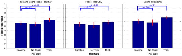
Memory performance on the final test (operationalized as the percentage of items where both category and item responses were correct), as a function of condition. Left panel: data for face trials and scene trials combined; middle panel: data for face trials only; right panel: data for scene trials only. Error bars indicate the SEM. Within each panel, think and no-think memory performance were compared to baseline using an across-subjects paired t-test.

3.2. fMRI results

3.2.1. Basic sensitivity analyses

Before launching into our curve-fitting analyses, we wanted to assess how sensitive the classifier was (overall) to scene and face information in different phases of the experiment. Figure 6 shows how well the difference in scene and face classifier evidence discriminated between face trials and scene trials in the functional localizer phase (where participants viewed faces and scenes), think trials (where participants were trying to remember picture associates, some of which were faces and some of which were scenes), and no-think trials (where participants were trying not to remember picture associates, some of which were faces and some of which were scenes). The figure shows that, not surprisingly, classifier sensitivity to the face/scene distinction was highest for the functional localizer, next-highest for think trials, and lowest for no-think trials. Crucially, classifier sensitivity was significantly above chance in all three conditions, including the no-think condition; that is, we were able to decode (with above-chance sensitivity) the category of the picture associate, even on trials where participants were specifically instructed not to retrieve the associate. The fact that classifier sensitivity was above chance in the no-think condition licensed us to explore (in our curve-fitting analyses, described below) how classifier evidence on no-think trials related to memory performance on the final test.

Figure 6.

Scene vs. face classification for the functional localizer, think trials, and no-think trials. Sensitivity was indexed using area under the ROC (AUC); the red line indicates chance performance (AUC = .5). AUC was computed separately for each condition within each participant. Error bars indicate the SEM. * indicates that sensitivity in that condition was significantly above chance according to an across-subjects t-test, p ≤ .001.

3.2.2. Event-related averages

Figure 7 shows average face and scene classifier evidence for the first 7 scans of think and nothink trials, as a function of whether the associate was a scene or a face. Each scan lasted two seconds, and scan 1 corresponds to the onset of the cue word. In addition to showing face and scene classifier evidence, the figure also shows the difference between classifier evidence for the “correct” category (i.e., the category of the associated memory) and the “incorrect” category. For each time point in each condition, we compared this “correct - incorrect classifier difference” measure to zero using an across-subjects t-test.

Figure 7.

Event-related averages of face and scene classifier evidence for the first 7 scans of think and no-think trials, split by whether the associate was a face (left side) or scene (right side). Each scan lasted 2 seconds. Dif = difference between classifier evidence for the correct vs. incorrect category. The ribbon around the dif line indicates the SEM. * indicates that dif was significantly greater than zero at that time point according to an across-subjects t-test, p < .05.

For think trials, classifier evidence for the correct category rose above classifier evidence for the incorrect category for both faces and scenes. For both categories, this difference was numerically maximal (and statistically significant, across participants) at scan 4, which is the scan that we used to read out memory retrieval strength for our curve-fitting analyses (see Section 2.5.4).

For no-think trials, the difference between correct-category and incorrect-category classifier evidence rose significantly above zero for scenes (as with scene think trials, the difference was numerically maximal and statistically significant at scan 4). However, there was no apparent difference between correct-category and incorrect-category classifier evidence on no-think face trials. Overall, these results suggest that we were receiving a useful memory signal on scene but possibly not on face no-think trials, and thus it might be useful to focus our curve-fitting analysis on scene no-think trials. We return to this point later in the Results section and in the Discussion section.

The event-related averages also show that there was considerable shared variance between correct-category and incorrect-category classifier evidence over the course of a trial; the memory effect was a small difference riding on top of this nonspecific effect. Based on this information, we opted to use the difference in correct vs. incorrect category evidence as our trial-by-trial measure of memory retrieval in our curve-fitting analyses, as opposed to looking just at the classifier evidence corresponding to the correct category. Looking at the difference should reduce the influence of non-memory-specific factors that affect both correct-category and incorrect-category classifier evidence values in tandem. ⁸

3.2.3. Curve-fitting analyses

Figure 8 shows the results of our curve-fitting procedure when it was applied to no-think data from all no-think trials (mixing together scene trials and face trials). The posterior probability of theory-consistency, P(theory consistent), was computed to be .51 in this analysis, indicating that the algorithm was almost perfectly uncertain about whether the underlying curve was theory-consistent. ⁹

Figure 8.

Results from our curve-fitting procedure, applied to data from all no-think trials (regardless of the category of the associated image). The dark line in the figure indicates the mean of the posterior distribution over curves, and the gray ribbon indicates the 90% credible interval (i.e., 90% of the probability mass is contained within the gray ribbon).

As stated above (see Figure 7), classifier evidence was reliably greater for scenes than faces on scene no-think trials, but – on face no-think trials – scene and face classifier evidence were indistiguishable from one another on average. One possible explanation for our poor initial curve-fitting results is that the classifier was not providing a useful index of memory retrieval on face trials, and the lack of good “signal” on these face trials was preventing the curve-fitting algorithm from uncovering the true underlying shape of the curve.

To address this issue, we ran the curve-fitting analysis separately on scene and face trials – if face trials were dragging down the overall P(theory consistent) value, then the results should be better when we focus just on scene trials. The results are shown in Figure 9. For faces, P(theory consistent) was low (0.40), but for scenes P(theory consistent) was substantially higher (0.76) and the recovered curve showed a pronounced U shape. ¹⁰

Figure 9.

Results from our curve-fitting procedure, applied to data from no-think trials with scene associates (on the left) and face associates (on the right). In both figures, the dark line indicates the mean of the posterior distribution over curves, and the gray ribbon indicates the 90% credible interval (i.e., 90% of the probability mass is contained within the gray ribbon).

Given that the scene results were more promising, we asked: What are the odds of getting a result this good due to chance? To test this, we ran a nonparametric permutation test (see Section 2.7.6). This permutation analysis yielded an empirical null distribution of P(theory consistent) values – this is the distribution that we would expect to observe if there were no real relationship between brain activity and behavior. This empirical null distribution is shown in Figure 10, along with the actual P(theory consistent) value. Out of 1000 samples in the null distribution, only 6 samples from the null showed a P(theory consistent) value greater than the actual P(theory consistent) value of .76. This finding suggests that it is very unlikely that we would have obtained a theory-consistency value this high due to chance (p < .01).

Figure 10.

Results of a permutation test of the P(theory consistent) value obtained for no-think, scene trials. The blue bars indicate the empirical null distribution of P(theory consistent) values, generated under the null hypothesis that there was no real relationship between brain activity and behavior. The green dot indicates the value of P(theory consistent) that was actually observed for no-think, scene trials. 6 out of 1000 permuted samples yielded a P(theory consistent) value greater than the actually observed value.

Readers will note that the mean of the computed null distribution was above .5, indicating a potential bias in the null toward theory consistency; this is especially surprising, given the fact – noted earlier – that theory-consistent curves occupy less than half of the total curve volume: 38.5%. This property of the null distribution is a consequence of our use of a very conservative permutation-testing procedure. As mentioned in Section 2.7.6, we permuted the behavioral memory outcome column within each condition (no think, baseline) within each participant, thereby ensuring that the overall level of memory performance within each condition within each participant was not affected by the permutation. A drawback of this procedure is that, if all of the behavioral memory outcomes within a participant/condition combination are the same (e.g., a particular participant correctly remembered all no-think items), then the permutation procedure will not change the data for that participant/condition. If the data do not change, this has the effect of pulling the null distribution towards the real data, thereby making it harder to obtain a significant difference between the real data and the null distribution. The fact that we obtained a highly significant effect despite this issue testifies to the strength of the effect. ¹¹

As noted in the Section 2.7.6, the permutation analysis permits inferences about the particular set of participants that we studied but not the population as a whole. To estimate the across-subject reliability of our results, we ran a bootstrap resampling analysis. For this analysis, we ran 1000 pseudoreplications of the experiment by sampling with replacement from our pool of 26 participants. Figure 11 shows the distribution of theory-consistency values that we obtained across the 1000 pseudoreplications. Crucially, we found that 95% (947 out of 1000) of the pseudoreplications showed theory-consistency values above .5 (indicating a balance of evidence in favor of our theory). These results suggest that, if we re-ran the experiment with new participants sampled from the same population, the odds are very high that we would obtain evidence consistent with our theory.

Figure 11.

Results of a bootstrap test assessing the across-participant reliability of the no-think, scene results. Green bars indicate the distribution of P(theory consistent) values obtained by running 1000 pseudoreplications of the experiment. For each pseudoreplication, we sampled 26 participants with replacement from our actual set of 26 participants, and we re-computed P(theory consistent). 947 out of 1000 pseudoreplications had P(theory consistent) values greater than .5.

4. Discussion

By applying pattern classifiers to fMRI data, we were able to derive a trial-by-trial readout of memory retrieval on no-think trials. We used this readout of the neural activity to predict subsequent memory for no-think items, and we found that the relationship between activation and subsequent memory was nonmonotonic for scene trials: Moderate activity of no-think scenes was associated with subsequent forgetting, but higher and lower levels of scene activity were not associated with forgetting (for discussion of scene/face differences see Section 4.3 below). While there have been many other fMRI studies of the think/no-think paradigm (Anderson et al., 2004; Depue et al., 2007; Levy & Anderson, 2012; Butler & James, 2010; Depue et al., 2010; Huddleston & Anderson, in preparation), ours is the first to use pattern classifiers to track memory activation, and it is the first to look for (and find) a nonmonotonic relationship between memory activation and learning.

4.1. Related results

The findings from this study converge with other results from our lab showing a relationship between moderate levels of brain activity (as measured by a classifier) and subsequently reduced performance. Apart from the present study, we have completed two experiments showing this pattern: a priming study (Newman & Norman, 2010) and a study looking at the effects of switching items into and out of working memory (Lewis-Peacock & Norman, 2012); both of these studies are briefly described below.

In the Newman & Norman (2010) priming study, participants were presented with two stimuli at once (e.g., a red-tinted face and a grayscale shoe) and they were asked to attend to the red-tinted stimulus while ignoring the grayscale stimulus. On a subset of trials (ignored repetition trials), participants were then asked to respond to the stimulus that they just ignored. Based on the nonmonotonic plasticity hypothesis, Newman & Norman (2010) predicted that the effect of ignoring the grayscale distractor on subsequent reaction time to that item would be U-shaped: Moderate levels of distractor processing should lead to weakening of the representation and thus slower responding (a negative priming effect; Tipper, 1985), whereas higher levels of distractor processing should lead to strengthening of the representation and thus faster responding (a positive priming effect). To test this prediction, Newman & Norman (2010) used category-specific pattern classifiers, applied to EEG data, to measure – on a trial-by-trial basis – the degree to which participants were processing the to-be-ignored stimulus during the initial display (e.g., if the distractor was a house, we would use the house classifier to track distractor processing). As predicted, Newman & Norman (2010) found a U-shaped relationship between distractor processing (as measured by the classifier) and subsequent reaction time: Low levels of distractor processing did not result in priming; moderate distractor processing led to a robust negative priming effect; and higher levels of distractor processing led to a (non-significant) hint of positive priming. Importantly, the overall difference in reaction time between ignored repetition trials and control trials (aggregating across all trials) was not significant – as in our think-no think experiment, clear evidence for inhibition only emerged when we used a pattern classifier to identify trials with moderate activation.

In the Lewis-Peacock & Norman (2012) study, we explored the long-term consequences of unloading items from working memory. When an item goes from being strongly active in working memory to being inactive, it necessarily has to pass through the “moderately active” zone. If, for whatever reason, a memory happens to linger in this moderately active zone while it is being unloaded from working memory, then – according to the nonmonotonic plasticity hypothesis – the memory will be weakened, making it harder to retrieve in the future. To test this prediction, we used a working memory switching paradigm. At the start of each trial, a face and a scene were briefly presented, followed by a delay. On 2/3 of the trials, participants were given a match-to-sample test for the scene at the end of the delay period. However, on the remaining 1/3 of the trials, the scene test was replaced by a switch cue instructing the participants that (after another delay) they would be tested on the face, not the scene; based on prior work, we hypothesized that the switch cue would result in participants loading the face into working memory and unloading the scene from working memory (Lewis-Peacock & Postle, 2012). Finally, at the end of the experiment, we gave participants a surprise memory test for the scenes that they viewed on switch trials – our main interest was in relating the dynamics of unloading scenes from working memory (during switch trials) to recognition memory for those scenes on the final test. We used a classifier to measure scene activity during switch trials, and we found that lingering activation of scene representations after the switch cue was associated with worse subsequent memory for those scenes. This result is somewhat counterintuitive (in the sense that more scene activation was associated with worse subsequent memory) but it fits with our theory of learning, which posits that sustained moderate (vs. low) activation can damage a memory.

It is worth noting that the think/no-think study, the Newman & Norman (2010) negative-priming study, and the Lewis-Peacock & Norman (2012) working-memory-switching study probed memory in very different ways: The think/no-think study tested memory for intentionally studied paired-associates from long-term memory; the Newman & Norman (2010) study looked at short-term reaction-time priming effects; and the Lewis-Peacock & Norman (2012) study looked at recognition memory for individual scenes after incidental study. The fact that all three paradigms showed a similar pattern fits with the idea that nonmonotonic plasticity is a general principle of learning that applies across multiple time scales and dependent measures. In ongoing work, we are looking for nonmonotonic effects across an even wider range of paradigms (e.g., statistical learning; see Section 4.2).

In addition to our lab’s neuroimaging studies, we should also mention a recent behavioral study by Keresztes & Racsmany (2012) that found a nonmonotonic relationship between interference and forgetting using a variant of the retrieval practice paradigm (Anderson et al., 1994). In this experiment, participants studied paired associates; next, they practiced retrieving a subset of these paired associates; finally, their memory was tested for practiced pairs as well as other items that were related or unrelated to the practiced pairs. Crucially, instead of measuring the activation of competing items (during retrieval practice) using a neuroimaging pattern classifier, Keresztes & Racsmany (2012) used participants’ reaction time during the retrieval practice trial as a proxy for the activation of competing items (long reaction time = high activation). As predicted by our theory, Keresztes & Racsmany (2012) found that moderate reaction times during retrieval practice (indicating moderate activation of competing items) led to more retrieval-induced forgetting of competing items than higher or lower reaction times. This study demonstrates that it is possible to map out a nonmonotonic plasticity curve using behavior alone, if you have a sufficiently sensitive behavioral measure of competition and sufficiently well-controlled stimuli.

4.2. Role of cognitive control

As noted in the Introduction, the observed U-shaped pattern is predicted both by the nonmonotonic plasticity hypothesis (Bienenstock et al., 1982; Diederich & Opper, 1987; Gardner, 1988; Senn & Fusi, 2005; Vico & Jerez, 2003; Norman et al., 2006a, 2007) and also by the executive control hypothesis (see, e.g., Levy & Anderson, 2002; Anderson & Levy, 2010). Importantly, both theories posit a role for cognitive control in driving memory weakening; the key difference between theories is whether this role is direct or indirect. According to the executive control hypothesis, successful application of cognitive control during the no-think phase is necessary and sufficient to trigger memory weakening. By contrast, the nonmonotonic plasticity hypothesis posits that the key underlying determinant of whether memories are strengthened or weakened is the degree of activation of the memory (i.e., is it low, moderate, or high), and that cognitive control processes indirectly affect learning by affecting the level of activation of competing memories. For example, in the think/no-think paradigm, cognitive control processes can boost forgetting by taking an item that would normally fall in the high-activation (strengthening) region of the curve and pushing it down into the moderate-activation (weakening) region of the curve. Since both theories predict a relationship between cognitive control and learning, both theories are equally compatible with extant neuroimaging findings showing a relationship between the activation of “cognitive control” regions (e.g., in prefrontal cortex) and forgetting of no-think items (e.g., Anderson et al., 2004; Depue et al., 2007).

One potential way to tease apart the theories is to look for nonmonotonic effects in paradigms that do not load heavily on cognitive control. The nonmonotonic plasticity hypothesis predicts that – if we could engineer a situation where a memory activates moderately in the absence of intentional suppression – forgetting should still occur. We are currently testing this hypothesis using a statistical learning paradigm where participants view a stream of faces and scenes and make simple judgments about these items (male/female for faces; indoor/outdoor for scenes; Kim et al., 2012). Previous studies of statistical learning have demonstrated that people make implicit predictions based on previously experienced statistical regularities – for example, if scene A was followed by face B the first time it appeared, then participants might implicitly predict face B when scene A is viewed again (see, e.g., Turk-Browne et al., 2010). If participants make an implicit prediction that is not confirmed, the predicted representation may end up with a moderate level of activation, leading to weakening of the memory. The statistical learning paradigm does not completely eliminate demands on cognitive control processes, but it does rely much less on intentional suppression than the paradigms we have explored up to this point (e.g., think/no-think, negative priming). As such, a successful demonstration of nonmonotonic plasticity in this paradigm would provide incremental support for the idea that “inhibitory” memory effects can occur without intentional suppression.

4.3. Differences between scenes and faces

In our curve-fitting analysis, we obtained strong evidence for the predicted U-shaped relationship between no-think classifier activity and memory performance on scene trials, but not on face trials. We think this difference may be a consequence of the classifier being more sensitive to scene activity than face activity on no-think trials. As reported in Figure 7, scene classifier evidence reliably exceeded face classifier evidence on scene no-think trials, but there was no reliable difference between face and scene classifier evidence on face no-think trials. ¹² The difference between theory-consistent and theory-inconsistent curves can be quite subtle – to the extent that scenes generate a “higher-fidelity” classifier signal, this may have given us the extra resolution that was required to discriminate between theory-consistent curves and (highly similar) theory-inconsistent curves (see the Supplementary Materials for simulations showing how measurement noise can result in theory-consistent curves being mistaken for theory-inconsistent curves, or vice-versa).

Results from the functional localizer phase provide converging support for the idea that (in our study) classifier sensitivity was higher for scenes than for faces. During the functional localizer, the average difference in correct-category vs. incorrect-category classifier evidence was larger when participants viewed scenes (scene evidence = .41; face evidence = −.15; difference = .56, SEM = .02) than when they viewed faces (face evidence = .32; scene evidence = −.15; difference = .47, SEM = .02), p < .005 according to an across-subjects paired t-test. Furthermore, a recent fMRI study by Reddy et al. (2010) suggests that this principle (i.e., places being more detectable than faces in fMRI data) may extend to other paradigms. As in our study, Reddy et al. (2010) trained their classifier on periods of time when participants were viewing categorized images (in their study, they used famous faces, famous buildings, tools, and food), using voxels from ventral-temporal cortex; they then applied the trained classifier to periods of time when participants were imagining items from those categories. In this “perception to imagery” condition, they found that single-trial classification accuracy for place (i.e., building) decoding was substantially higher than single-trial accuracy for face decoding.

4.4. Using category-specific activity to track item retrieval

In the analyses described above, we used category-specific activation (as measured by the classifier) as an index of how strongly individual items were being retrieved. Our preferred explanation of the observed association between moderate levels of classifier evidence and forgetting is that 1) moderate levels of classifier evidence reflect moderate levels of memory activation, and 2) moderate levels of memory activation result in memory weakening. However, alternative accounts of this finding are possible. For example, it is possible that moderate levels of classifier evidence could reflect strong activation of generic scene information, as opposed to moderate activation of specific scene information. We know from prior studies that the parahippocampal place area (PPA) responds strongly to layout information (Epstein & Kanwisher, 1998; Epstein et al., 1999); if the participant strongly retrieves the idea that “this word was linked to a bedroom scene”, but no specific layout information, this could result in moderate PPA activation and (through this) moderate output of the scene classifier. If participants form a new association between the word cue and the (retrieved) generic scene information, this new association could interfere with retrieval of the old association at test, thereby explaining the observed linkage between moderate levels of classifier evidence (here, interpreted as strong generic scene retrieval) and forgetting on the final test. ¹³

Fortunately, it is possible to arbitrate between our preferred interpretation of the data and this alternative interpretation by relating classifier output to (behavioral) category memory accuracy. Our preferred hypothesis (i.e., moderate classifier output reflects moderate activation of both category and item information) implies that moderate classifier output should be associated with forgetting of both category and item information. In this case, we should see the same nonmonotonic curve (showing a linkage between moderate classifier output and forgetting) when we relate classifier output to behavioral category memory accuracy. By contrast, the alternative hypothesis (i.e., moderate classifier output reflects strong activation of category information, and weak activation of item information) implies that moderate classifier output should be associated with improved category memory (since, by hypothesis, the category representation is strongly activated, and strong activation leads to further memory strengthening).

To address this question, we ran an analysis relating classifier evidence on scene trials to category memory accuracy. The shape of the resulting curve was qualitatively identical to the shape that we observed in our primary analyses relating classifier evidence on scene trials to item memory accuracy; crucially, moderate levels of classifier evidence were associated with forgetting of category activation. This result supports our preferred interpretation of moderate classifier evidence (i.e., that it reflects moderate overall activation) and goes against the alternative explanation described above. ¹⁴

4.5. Interpreting unscaled classifier evidence values

Before feeding the classifier evidence values into the curve-fitting algorithm, we computed the difference between correct-category and incorrect-category classifier evidence, and we scaled these difference scores to fit within a 0-to-1 range. Both steps are important: Taking the difference between correct-category and incorrect-category evidence corrects for nonspecific factors (e.g., task engagement) that affect classifier evidence for both categories in tandem, and scaling is necessary to get the curve-fitting algorithm to work (since the algorithm expects 0-to-1 x values). However, scaling has the drawback of obscuring the actual classifier evidence values.

To gain further insight into what the classifier is doing, we can look at the unscaled classifier evidence values: For the “scene-only” curve-fitting analysis shown in Figure 9, the minimum scene – face classifier evidence value was −.62 and the maximum value was .77; these values were mapped onto zero and one, respectively, on the x-axis of the scaled curve. The minimum y-value on the scene-only plasticity curve (the “dip”) corresponds to an unscaled scene – face value of −.31. Up to this point, we have been interpreting the left side of the scene-only plasticity curve (from the leftmost edge to the dip) as reflecting low-to-moderate levels of scene recall. However, the unscaled scores – showing greater face evidence than scene evidence on these trials – suggest that participants may be incorrectly recalling faces (or possibly items from other categories) on these trials.

While we can not rule this out, there are two important reasons to be skeptical of this interpretation. First, we should note that face classifier evidence and scene classifier evidence are not pure indices of face and scene processing, respectively. As reported above in Section 4.3, the face classifier shows a characteristic negative deflection when participants view scenes during the functional localizer, and the scene classifier shows a characteristic negative deflection when participants view faces during the functional localizer; other studies have found a similar “push-pull” relationship between face-specific and scene-specific processing regions (e.g., Gazzaley et al., 2005). To the extent that this push-pull relationship exists during no-think trials, low levels of scene processing could be expressed both as low levels of activity in scene-specific regions and high levels of activity in face-specific regions, resulting in negative scene – face classifier evidence scores. Second, if we interpret the left side of the scene-only plasticity curve as reflecting varying degrees of face recall (such that face recall is highest at the left edge, and somewhat lower at the point of the dip), it is unclear why the dip occurs. Why should high levels of face recall on no-think trials lead to better subsequent scene memory than moderate levels of face recall? If anything, higher levels of face recall should predict worse subsequent scene memory on the final test.

4.6. Limitations and future directions

Fostering low-to-moderate activation

While the nonmonotonicity in the plasticity curve was statistically reliable, our curve-fitting results still reflect considerable uncertainty about the precise shape of the plasticity curve. In large part, this residual uncertainty is due to undersampling of key regions of “memory activation space”. Pooling across all no-think trials from all participants, the shape of the distribution of classifier evidence scores is Gaussian, with greater density in the middle than on the edges; this undersampling of the edges is evident in the credible intervals in Figure 8 and Figure 9, which bulge outward (indicating greater uncertainty) on the left and right edges of the plot. Undersampling of the edges is problematic for our estimation procedure, insofar as the left edge of the curve is the part that distinguishes theory consistent curves from (theory-inconsistent) monotonically increasing curves. One way to address this problem is to include conditions that are specifically aimed at sampling the low-to-moderate activation range. For example, in the Lewis-Peacock & Norman (2012) working-memory-switching study, we measured scene activity for several seconds after the scene was deemed to be irrelevant on that trial; in this situation, where nothing was onscreen cuing the scene, the resulting levels of classifier evidence ranged from very low to moderate (relative to parts of the trial where participants were actively maintaining the scene).

Another way to address this undersampling problem is to move toward adaptive real-time fMRI procedures, where we measure memory activation using pattern classifiers and then dynamically adjust the parameters of the experiment to increase the odds that memory activation will fall within the “dip” of the plasticity curve. For example, if we observe that a particular cue is eliciting too much memory activation (leading to strengthening), we could present the cue more briefly on the next trial, which hopefully will reduce the amount of memory activation elicited by the cue. We have adaptive studies of this sort underway now in our lab. If we devise a paradigm that reliably elicits moderate activation (using fMRI neurofeedback) this could be used to enact targeted weakening of undesirable memories (e.g., in PTSD patients).

Linking back to neurophysiology

This research was motivated by the well-established U-shaped function relating the depolarization of postsynaptic neurons to long-term potentiation and depression (Artola et al., 1990; Hansel et al., 1996). This U-shaped synaptic plasticity function is a possible explanation of the results reported here; according to this hypothesis, when a scene memory activates moderately (as indicated by the classifier), the neurons representing the scene memory are moderately depolarized, resulting in long-term depression (i.e., weakening) of the synapses underlying that memory. The current dataset does not allow us to assess whether this explanation is correct – our fMRI measure is several steps removed from neural firing, and there is no guarantee that moderate classifier output corresponds to moderate post-synaptic depolarization. In future work, we plan to extend this research to other imaging modalities (e.g., multi-unit electrophysiology) that provide a more resolved picture of neural activity; this will allow us to more definitively assess the relationship between the cognitive-level phenomena discussed here and the synaptic mechanisms described by Artola et al. (1990) and others.

4.7. Conclusions

In summary, we used a Bayesian curve-fitting procedure (described here for the first time) to demonstrate a nonmonotonic relationship between the activation of scene memories on no-think trials and subsequent memory for these scenes on the final memory test: Moderate activation of no-think scenes led to forgetting but higher and lower levels did not. From a practical perspective, this nonmonotonic relationship helps to explain why some studies have failed to observe significant forgetting of no-think items. From a theoretical perspective, these results are consistent with neural network models positing that moderate activation leads to synaptic weakening (e.g., Norman et al., 2006a, 2007) and also with theories positing that memory inhibition is caused by successful (but not unsuccessful) application of cognitive control (Anderson & Levy, 2010). Researchers interested in pursuing these kinds of analyses (i.e., assessing the shape of the relationship between memory activation and subsequent memory) are encouraged to download our P-CIT curve-fitting toolbox from http://code.google.com/p/p-cit-toolbox/.

• We used pattern classifiers to measure memory activation in a think/no-think study.

• We estimated how memory activation on no-think trials related to subsequent recall.

• This relationship was estimated using a novel Bayesian importance sampling algorithm.

• The relationship between activation and subsequent recall was found to be U-shaped.

References

- Anderson M, Levy B. Suppressing unwanted memories. Current Directions in Psychological Science. 2009;18:189–194. doi: 10.1177/0963721417689881. [DOI] [PMC free article] [PubMed] [Google Scholar]
- Anderson MC, Bjork RA, Bjork EL. Remembering can cause forgetting: retrieval dynamics in long-term memory. Journal of Experimental Psychology: Learning, Memory, and Cognition. 1994;20:1063–1087. doi: 10.1037//0278-7393.20.5.1063. [DOI] [PubMed] [Google Scholar]
- Anderson MC, Green C. Suppressing unwanted memories by executive control. Nature. 2001;410:366–369. doi: 10.1038/35066572. [DOI] [PubMed] [Google Scholar]
- Anderson MC, Huddleston E. Towards a cognitive and neurobiological model of motivated forgetting. In: Belli RF, editor. True and False Recovered Memories. Springer; 2012. pp. 53–120. [DOI] [PubMed] [Google Scholar]
- Anderson MC, Levy BJ. On the relationship between interference and inhibition in cognition. In: Benjamin AS, editor. Successful remembering and successful forgetting: a festschrift in honor of Robert A Bjork. Psychology Press; 2010. pp. 107–132. [Google Scholar]
- Anderson MC, Ochsner KN, Kuhl B, Cooper J, Robertson E, Gabrieli SW, Glover GH, Gabrieli JD. Neural systems underlying the suppression of unwanted memories. Science. 2004;303:232–235. doi: 10.1126/science.1089504. [DOI] [PubMed] [Google Scholar]
- Anderson MC, Reinholz J, Kuhl BA, Mayr U. Intentional suppression of unwanted memories grows more difficult as we age. Psychology & Aging. 2011;26:397–405. doi: 10.1037/a0022505. [DOI] [PubMed] [Google Scholar]
- Artola A, Brocher S, Singer W. Different voltage-dependent thresholds for inducing long-term depression and long-term potentiation in slices of rat visual cortex. Nature. 1990;347:69–72. doi: 10.1038/347069a0. [DOI] [PubMed] [Google Scholar]
- Bauml KH, Hanslmayr S. Forgetting in the no-think paradigm: interference or inhibition? Proceedings of the National Academy of Sciences USA. 2010;107:E3. doi: 10.1073/pnas.0912576107. [DOI] [PMC free article] [PubMed] [Google Scholar]
- Bear M. Bidirectional synaptic plasticity: from theory to reality. Philosophical Transactions of the Royal Society of London Series B: Biological Sciences. 2003;358:649–655. doi: 10.1098/rstb.2002.1255. [DOI] [PMC free article] [PubMed] [Google Scholar]
- Benoit RG, Anderson MC. Opposing mechanisms support the voluntary forgetting of unwanted memories. Neuron. 2012;76:450–460. doi: 10.1016/j.neuron.2012.07.025. [DOI] [PMC free article] [PubMed] [Google Scholar]
- Bergström Z, de Fockert J, Richardson-Klavehn A. ERP and behavioural evidence for direct suppression of unwanted memories. NeuroImage. 2009;48:726–737. doi: 10.1016/j.neuroimage.2009.06.051. [DOI] [PubMed] [Google Scholar]
- Bergström ZM, Velmans M, de Fockert J, Richardson-Klavehn A. ERP evidence for successful voluntary avoidance of conscious recollection. Brain Research. 2007;1151:119–33. doi: 10.1016/j.brainres.2007.03.014. [DOI] [PubMed] [Google Scholar]
- Bienenstock EL, Cooper LN, Munro PW. Theory for the development of neuron selectivity: Orientation specificity and binocular interaction in visual cortex. Journal of Neuroscience. 1982;2:32–48. doi: 10.1523/JNEUROSCI.02-01-00032.1982. [DOI] [PMC free article] [PubMed] [Google Scholar]
- Bulevich JB, Roediger HL, Balota DA, Butler AC. Failures to find suppression of episodic memories in the think/no-think paradigm. Memory & Cognition. 2006;34:1569–1577. doi: 10.3758/bf03195920. [DOI] [PubMed] [Google Scholar]
- Butler A, James K. The neural correlates of attempting to suppress negative versus neutral memories. Cognitive, Affective, & Behavioral Neuroscience. 2010;10:182–194. doi: 10.3758/CABN.10.2.182. [DOI] [PubMed] [Google Scholar]
- Cox RW. AFNI: software for analysis and visualization of functional magnetic resonance neuroimages. Computers and Biomedical Research. 1996;29:162–173. doi: 10.1006/cbmr.1996.0014. [DOI] [PubMed] [Google Scholar]
- Cox RW, Jesmanowicz A. Real-time 3d image registration for functional MRI. Magnetic Resonance in Medicine. 1999;42:1014–1018. doi: 10.1002/(sici)1522-2594(199912)42:6<1014::aid-mrm4>3.0.co;2-f. [DOI] [PubMed] [Google Scholar]
- Depue B, Burgess G, Willcutt E, Ruzic L, Banich M. Inhibitory control of memory retrieval and motor processing associated with the right lateral prefrontal cortex: Evidence from deficits in individuals with ADHD. Neuropsychologia. 2010;48:3909–3917. doi: 10.1016/j.neuropsychologia.2010.09.013. [DOI] [PMC free article] [PubMed] [Google Scholar]
- Depue BE. A neuroanatomical model of prefrontal inhibitory modulation of memory retrieval. Neuroscience and Biobehavioral Reviews. 2012;36:1382–1399. doi: 10.1016/j.neubiorev.2012.02.012. [DOI] [PMC free article] [PubMed] [Google Scholar]
- Depue BE, Curran T, Banich MT. Prefrontal regions orchestrate suppression of emotional memories via a two-phase process. Science. 2007;317:215–219. doi: 10.1126/science.1139560. [DOI] [PubMed] [Google Scholar]
- Detre G, Polyn SM, Moore CD, Natu VS, Singer BD, Cohen JD, Haxby JV, Norman KA. The Multi-Voxel Pattern Analysis (MVPA) toolbox. Poster presented at the Annual Meeting of the Organization for Human Brain Mapping.2006. [Google Scholar]
- Diederich S, Opper M. Learning of correlated patterns in spin-glass networks by local learning rules. Physical Review Letters. 1987;58:949–952. doi: 10.1103/PhysRevLett.58.949. [DOI] [PubMed] [Google Scholar]
- Efron B, Tibshirani R. Bootstrap methods for standard errors, confidence intervals, and other measures of statistical accuracy. Statistical Science. 1986;1:54–75. [Google Scholar]
- Epstein R, Harris A, Stanley D, Kanwisher N. The parahippocampal place area: recognition, navigation, or encoding? Neuron. 1999;23:115–125. doi: 10.1016/s0896-6273(00)80758-8. [DOI] [PubMed] [Google Scholar]
- Epstein R, Kanwisher N. A cortical representation of the local visual environment. Nature. 1998;392:598–601. doi: 10.1038/33402. [DOI] [PubMed] [Google Scholar]
- Fawcett T. An introduction to ROC analysis. Pattern Recognition Letters. 2006;27:861–874. [Google Scholar]
- Friendly M, Franklin P, Hoffman D, Rubin D. The toronto word pool: Norms for imagery, concreteness, orthographic variables, and grammatical usage for 1,080 words. Behavior Research Methods. 1982;14:375–399. [Google Scholar]
- Gardner E. The space of interactions in neural network models. Journal of Physics A: Mathematical and General. 1988;21:257–270. [Google Scholar]
- Gazzaley A, Cooney JW, McEvoy K, Knight RT, D’Esposito M. Top-down enhancement and suppression of the magnitude and speed of neural activity. Journal of Cognitive Neuroscience. 2005;17:507–517. doi: 10.1162/0898929053279522. [DOI] [PubMed] [Google Scholar]
- Gelman A, Carlin J, Stern H, Rubin D. Bayesian Data Analysis. Chapman and Hall; 2004. [Google Scholar]
- Gotts SJ, Plaut DC. Neural mechanisms underlying positive and negative repetition priming. Poster presented at the Annual Meeting of the Cognitive Neuroscience Society.2005. [Google Scholar]
- Hansel C, Artola A, Singer W. Different threshold levels of postsynaptic [Ca2+]i have to be reached to induce LTP and LTD in neocortical pyramidal cells. Journal of Physiology (Paris) 1996;90:317–319. doi: 10.1016/s0928-4257(97)87906-5. [DOI] [PubMed] [Google Scholar]
- Hastie T, Tibshirani R, Friedman J. The Elements of Statistical Learning. New York, NY: Springer; 2001. [Google Scholar]
- Haxby JV, Gobbini MI, Furey ML, Ishai A, Schouten JL, Pietrini P. Distributed and overlapping representations of faces and objects in ventral temporal cortex. Science. 2001;293:2425–2430. doi: 10.1126/science.1063736. [DOI] [PubMed] [Google Scholar]
- Haynes JD, Rees G. Decoding mental states from brain activity in humans. Nature Reviews Neuroscience. 2006;7:523–534. doi: 10.1038/nrn1931. [DOI] [PubMed] [Google Scholar]
- Hertel P, Mahan A. Depression-related differences in learning and forgetting responses to unrelated cues. Acta Psychologica. 2008;127:636–644. doi: 10.1016/j.actpsy.2007.11.004. [DOI] [PubMed] [Google Scholar]
- Hertel PT, Calcaterra G. Intentional forgetting benefits from thought substitution. Psychonomic Bulletin and Review. 2005;12:484–489. doi: 10.3758/bf03193792. [DOI] [PubMed] [Google Scholar]
- Hoerl A, Kennard R. Ridge regression: Biased estimation for nonorthogonal problems. Technometrics. 1970;12:55– 67. [Google Scholar]
- Holmes AP, Friston KJ. Generalisability, random effects and population inference. NeuroImage. 1998;7:S754. [Google Scholar]
- Huber D, Tomlinson T, Rieth C, Davelaar E. Reply to Bäuml and Hanslmayr: Adding or subtracting memories? The neural correlates of learned interference vs. memory inhibition. Proceedings of the National Academy of Sciences USA. 2010;107:E4–E4. [Google Scholar]
- Huddleston E, Anderson MC. Retrieval suppression modulates activation in content-specific neocortical areas. (in preparation) [Google Scholar]
- Keresztes A, Racsmany M. Interference resolution in retrieval-induced forgetting: Behavioral evidence for a nonmonotonic relationship between interference and forgetting. Memory and Cognition. 2012 doi: 10.3758/s13421-012-0276-3. [DOI] [PubMed] [Google Scholar]
- Kim G, Lewis-Peacock JA, Norman KA, Turk-Browne NB. Context-based prediction and memory suppression. Poster presented at the Society for Neuroscience Annual Meeting.2012. [Google Scholar]
- Kriegeskorte N, Simmons WK, Bellgowan PS, Baker CI. Circular analysis in systems neuroscience: the dangers of double dipping. Nature Neuroscience. 2009;12:535–540. doi: 10.1038/nn.2303. [DOI] [PMC free article] [PubMed] [Google Scholar]
- Kuhl BA, Bainbridge WA, Chun MM. Neural reactivation reveals mechanisms for updating memory. Journal of Neuroscience. 2012;32:3453–3461. doi: 10.1523/JNEUROSCI.5846-11.2012. [DOI] [PMC free article] [PubMed] [Google Scholar]
- Kuhl BA, Rissman J, Chun MM, Wagner AD. Fidelity of neural reactivation reveals competition between memories. Proceedings of the National Academy of Sciences USA. 2011;108:5903–5908. doi: 10.1073/pnas.1016939108. [DOI] [PMC free article] [PubMed] [Google Scholar]
- Lashkari D, Vul E, Kanwisher N, Golland P. Discovering structure in the space of fMRI selectivity profiles. Neuroimage. 2010;50:1085–1098. doi: 10.1016/j.neuroimage.2009.12.106. [DOI] [PMC free article] [PubMed] [Google Scholar]
- Levy BJ, Anderson MC. Inhibitory processes and the control of memory retrieval. Trends in Cognitive Sciences. 2002;6:299–305. doi: 10.1016/s1364-6613(02)01923-x. [DOI] [PubMed] [Google Scholar]
- Levy BJ, Anderson MC. Individual differences in the suppression of unwanted memories: the executive deficit hypothesis. Acta Psychologica. 2008;127:623–635. doi: 10.1016/j.actpsy.2007.12.004. [DOI] [PubMed] [Google Scholar]
- Levy BJ, Anderson MC. Purging of memories from conscious awareness tracked in the human brain. J Neurosci. 2012;32:16785–16794. doi: 10.1523/JNEUROSCI.2640-12.2012. [DOI] [PMC free article] [PubMed] [Google Scholar]
- Lewis-Peacock J, Norman KA. Deactivation of items in working memory can weaken long-term memory. Poster presented at the Cognitive Neuroscience Society Annual Meeting.2012. [Google Scholar]
- Lewis-Peacock JA, Postle BR. Temporary activation of long-term memory supports working memory. Journal of Neuroscience. 2008;28:8765–8771. doi: 10.1523/JNEUROSCI.1953-08.2008. [DOI] [PMC free article] [PubMed] [Google Scholar]
- Lewis-Peacock JA, Postle BR. Decoding the internal focus of attention. Neuropsychologia. 2012;50:470–478. doi: 10.1016/j.neuropsychologia.2011.11.006. [DOI] [PMC free article] [PubMed] [Google Scholar]
- MacKay D. Information theory, inference, and learning algorithms. Cambridge Univ Pr; 2003. [Google Scholar]
- McDuff SGR, Frankel HC, Norman KA. Multivoxel pattern analysis reveals increased memory targeting and reduced use of retrieved details during single-agenda source monitoring. Journal of Neuroscience. 2009;29:508–516. doi: 10.1523/JNEUROSCI.3587-08.2009. [DOI] [PMC free article] [PubMed] [Google Scholar]
- Mecklinger A, Parra M, Waldhauser G. ERP correlates of intentional forgetting. Brain Research. 2009;1255:132–147. doi: 10.1016/j.brainres.2008.11.073. [DOI] [PubMed] [Google Scholar]
- Munakata Y, Herd SA, Chatham CH, Depue BE, Banich MT, O’Reilly RC. A unified framework for inhibitory control. Trends in Cognitive Sciences. 2011;15:453–459. doi: 10.1016/j.tics.2011.07.011. [DOI] [PMC free article] [PubMed] [Google Scholar]
- Newman EL, Norman KA. Moderate excitation leads to weakening of perceptual representations. Cerebral Cortex. 2010;20:2760–2770. doi: 10.1093/cercor/bhq021. [DOI] [PMC free article] [PubMed] [Google Scholar]
- Nieuwenhuis S, Forstmann BU, Wagenmakers EJ. Erroneous analyses of interactions in neuroscience: a problem of significance. Nature Neuroscience. 2011;14:1105–1107. doi: 10.1038/nn.2886. [DOI] [PubMed] [Google Scholar]
- Norman KA, Newman EL, Detre G. A neural network model of retrieval-induced forgetting. Psychological Review. 2007;114:887–953. doi: 10.1037/0033-295X.114.4.887. [DOI] [PubMed] [Google Scholar]
- Norman KA, Newman EL, Detre GJ, Polyn SM. How inhibitory oscillations can train neural networks and punish competitors. Neural Computation. 2006a;18:1577–1610. doi: 10.1162/neco.2006.18.7.1577. [DOI] [PubMed] [Google Scholar]
- Norman KA, Polyn SM, Detre GJ, Haxby JV. Beyond mind-reading: Multi-voxel pattern analysis of fMRI data. Trends in Cognitive Sciences. 2006b;10:424–430. doi: 10.1016/j.tics.2006.07.005. [DOI] [PubMed] [Google Scholar]
- Paz-Alonso PM, Ghetti S, Matlen BJ, Anderson MC, Bunge SA. Memory suppression is an active process that improves over childhood. Frontiers in Human Neuroscience. 2009;3:24. doi: 10.3389/neuro.09.024.2009. [DOI] [PMC free article] [PubMed] [Google Scholar]
- Pereira F, Mitchell T, Botvinick M. Machine learning classifiers and fMRI: a tutorial overview. Neuroimage. 2009;45:199–209. doi: 10.1016/j.neuroimage.2008.11.007. [DOI] [PMC free article] [PubMed] [Google Scholar]
- Polyn SM, Natu VS, Cohen JD, Norman KA. Category-specific cortical activity precedes retrieval during memory search. Science. 2005;310:1963–1966. doi: 10.1126/science.1117645. [DOI] [PubMed] [Google Scholar]
- Poppenk J, Norman K. Mechanisms supporting superior source memory for familiar items: A multi-voxel pattern analysis study. Neuropsychologia. 2012 doi: 10.1016/j.neuropsychologia.2012.07.010. [DOI] [PMC free article] [PubMed] [Google Scholar]
- Raaijmakers JGW, Jakab E. Rethinking inhibition theory: On the problematic status of the inhibitory theory for forgetting. (submitted) [Google Scholar]
- Reddy L, Tsuchiya N, Serre T. Reading the mind’s eye: decoding category information during mental imagery. Neuroimage. 2010;50:818–825. doi: 10.1016/j.neuroimage.2009.11.084. [DOI] [PMC free article] [PubMed] [Google Scholar]
- Rissman J, Wagner AD. Distributed representations in memory: insights from functional brain imaging. Annual Review of Psychology. 2012;63:101–128. doi: 10.1146/annurev-psych-120710-100344. [DOI] [PMC free article] [PubMed] [Google Scholar]
- Senn W, Fusi S. Learning only when necessary: better memories of correlated patterns in networks with bounded synapses. Neural Computation. 2005;17:2106–2138. doi: 10.1162/0899766054615644. [DOI] [PubMed] [Google Scholar]
- Tipper SP. The negative priming effect: inhibitory priming by ignored objects. The Quarterly Journal of Experimental Psychology A, Human Experimental Psychology. 1985;37:571–590. doi: 10.1080/14640748508400920. [DOI] [PubMed] [Google Scholar]
- Tomlinson TD, Huber DE, Rieth CA, Davelaar EJ. An interference account of cue-independent forgetting in the no-think paradigm. Proceedings of the National Academy of Sciences USA. 2009;106:15588–15593. doi: 10.1073/pnas.0813370106. [DOI] [PMC free article] [PubMed] [Google Scholar]
- Tong F, Pratte MS. Decoding patterns of human brain activity. Annual Review of Psychology. 2012;63:483–509. doi: 10.1146/annurev-psych-120710-100412. [DOI] [PMC free article] [PubMed] [Google Scholar]
- Turk-Browne NB, Scholl BJ, Johnson MK, Chun MM. Implicit perceptual anticipation triggered by statistical learning. Journal of Neuroscience. 2010;30:11177–11187. doi: 10.1523/JNEUROSCI.0858-10.2010. [DOI] [PMC free article] [PubMed] [Google Scholar]
- Vico F, Jerez J. Stable neural attractors formation: Learning rules and network dynamics. Neural Processing Letters. 2003;18:1–16. [Google Scholar]
- Vul E, Lashkari D, Hsieh PJ, Golland P, Kanwisher N. Data-driven functional clustering reveals dominance of face, place, and body selectivity in the ventral visual pathway. Journal of Neurophysiology. 2012 doi: 10.1152/jn.00354.2011. [DOI] [PMC free article] [PubMed] [Google Scholar]
- Woods RP. Modeling for intergroup comparisons of imaging data. Neuroimage. 1996;4:84–94. doi: 10.1006/nimg.1996.0058. [DOI] [PubMed] [Google Scholar]
- Zeithamova D, Dominick AL, Preston AR. Hippocampal and ventral medial prefrontal activation during retrieval-mediated learning supports novel inference. Neuron. 2012;75:168–179. doi: 10.1016/j.neuron.2012.05.010. [DOI] [PMC free article] [PubMed] [Google Scholar]
Associated Data
This section collects any data citations, data availability statements, or supplementary materials included in this article.