Model for macroevolutionary dynamics

Significance

Genera are often viewed as artificial constructs of taxonomic practice. Here, we show that a stochastic model that includes three events with constant rates—species formation, extinction of species, and origination of new genera—can describe well the species-within-genus distributions for large taxa. Predictions from the model, including origination times of large taxa and origination rates of genera, match values obtained by other methods. Likewise, estimated extinction rates are close to speciation rates, which is consistent with the paleontological record. The model’s success emphasizes that, although taxonomic groupings are manmade, they nonetheless reflect natural evolutionary processes.

Abstract

The highly skewed distribution of species among genera, although challenging to macroevolutionists, provides an opportunity to understand the dynamics of diversification, including species formation, extinction, and morphological evolution. Early models were based on either the work by Yule [Yule GU (1925) Philos Trans R Soc Lond B Biol Sci 213:21–87], which neglects extinction, or a simple birth–death (speciation–extinction) process. Here, we extend the more recent development of a generic, neutral speciation–extinction (of species)–origination (of genera; SEO) model for macroevolutionary dynamics of taxon diversification. Simulations show that deviations from the homogeneity assumptions in the model can be detected in species-per-genus distributions. The SEO model fits observed species-per-genus distributions well for class-to-kingdom–sized taxonomic groups. The model’s predictions for the appearance times (the time of the first existing species) of the taxonomic groups also approximately match estimates based on molecular inference and fossil records. Unlike estimates based on analyses of phylogenetic reconstruction, fitted extinction rates for large clades are close to speciation rates, consistent with high rates of species turnover and the relatively slow change in diversity observed in the fossil record. Finally, the SEO model generally supports the consistency of generic boundaries based on morphological differences between species and provides a comparator for rates of lineage splitting and morphological evolution.

What we know about the diversification of life on earth comes primarily from two types of evidence: the fossil record and evolutionary relationships among contemporary taxa. Each of these sources is limited: the paleontological record is incomplete and often difficult to interpret, whereas inference about the past dynamics of a system from its current state depends on having suitable models. Given these limitations, it is not surprising that macroevolution still lacks a unifying paradigmatic framework. Of particular importance is the continuing debate about the relative importance of intrinsic biotic effects vs. extrinsic physical/geochemical factors (1).

Because of the bewildering complexity of biological systems, stochastic minimal models have become very important. A definition of minimal in this context would disregard both endogenous and exogenous effects; these models are neutral, providing no role for fitness or selection, and they are homogeneous with respect to speciation and extinction rates across species and over time. Predictions of such models can be compared with the gross features of a time series extracted from fossil data (2) or contemporary patterns of taxonomic richness (3).

Although the assumptions of neutrality and homogeneity are unrealistically strong, two considerations support the use of these minimal stochastic models. First, such models fill the classical negative role of the null hypothesis, namely to assess the need for an alternative explanation. Thus, the abundance of a particular species does not indicate its relative evolutionary success unless the species abundance distribution differs significantly from the outcome of a random birth–death process (4, 5). An interesting example is the great variation in abundance observed among surnames in human populations, which presumably has nothing to do with selective pressure against or for a certain last name but is the outcome of a simple stochastic process (6, 7).

Second, some elements of a null model may be more realistic than they seem at first glance. For example, although a species may be driven to extinction by a superior competitor possessing a favorable genetic mutation, a deterministic description of this process that assumes a fixed fitness for each species may be naïve. Many events, including climate change, invasion of other species, emergence of new pathogens, and favorable mutations, may change the rules of the game and even reverse relative evolutionary success. Deterministic processes, such as natural selection, are thus immersed in noisy environments dominated by random events. A fully stochastic model that neglects effects of selection indeed provides a plausible description of reality, at least in its broad outlines. Our aim here is to explore the implications of a minimal model for macroevolution based on a stochastic speciation–extinction–origination (SEO) process. The model’s predictions fit many distributions of the number of species within genera as well as other features associated with past dynamics of species evolution. Because the SEO model describes these data well, we suggest that it might serve as a standard null model of diversification in the first (negative) sense explained above.

Similar models have been developed in the past (8, 9) and applied recently to analyze taxonomically organized patterns of diversity (10). We compare these models and applications with our model below. In addition, whereas previous species-within-genus distributions (SGDs) were based on partial datasets, we have also reconstructed SGDs from the largest datasets currently available (http://www.sp2000.org/) (11), containing more than 1 million species (details in SI Appendix).

Based on these datasets, we consider whether the neutral homogenous SEO model is a plausible or semiplausible description of the evolutionary process. To this end, we use the correspondence between the SGD and the SEO process as an inference technique, showing, for example, that the origination times inferred for higher taxonomic groups match estimates based on molecular inference and fossil data.

The fact that the SEO model not only closely fits SGDs but also successfully infers diversification rates and origination times reinforces the validity of the genus as a morphologically recognized level in the taxonomic hierarchy. Such is the case, even though genera and species are subjective constructs of the taxonomists who describe species and infer their relationships. Thus, the borders defining genera are unlikely to be consistent among taxonomists or among taxonomic groups. However, unless taxonomic distinctions differ substantially for larger vs. smaller genera (e.g., a strong bias among taxonomists to making large genera smaller and small genera larger), such inconsistencies between taxonomists would only add to the underlying stochasticity of SGDs. SI Appendix shows a simulated demonstration of this point. A recent study showed a basic similarity between morphologically defined and DNA sequence-defined genera (12). Moreover, because new genera may arise within existing genera, some level of paraphyly is to be expected before lineages become sorted into reciprocally monophyletic relationships.

Of course, too much noise would make it impossible to model the system. However, there is no reason to assume that inconsistencies between taxonomists would have reached that threshold, especially when dealing with classifications within large taxa (e.g., kingdoms and classes), which are the creations of many individuals following diverse taxonomic muses over long periods. Individual biases in such a large system will tend to cancel each other. Furthermore, the fact that we are able to build a realistic model that fits the data well, as we will show, lends support to the use of the taxonomic system as a description of evolutionary diversification. If the actual diversification process differed strongly from the pattern suggested below, it is unlikely that the bias and the noise associated with classification practices would lead to such nice agreement between the theory and the data.

Even with the rise of modern phylogenetic analysis, the traditional taxonomic system is, in fact, still widely used. Thus, phylogenetic comparative studies regularly calculate features such as species richness, morphological diversity, and functional diversity for major lineages, which correspond to established taxonomic groups (13–16). Our model can shed light on the underlying evolutionary dynamics of this pervasive but poorly understood system.

Indeed, a taxonomy-based approach has certain advantages compared with phylogenetic approaches. New genera reflect a certain level of divergence from the traits of contemporary relatives; the origin or multiple origins of new genera within a clade can lead to paraphyly, multiple paraphyly, or even polyphyly of a morphologically circumscribed genus. This fact is part of the reality of evolution. Current molecular phylogenetic practices insist on monophyly of taxonomic entities, thereby artificially erasing a part of the evolutionary history of a clade. The SEO model is blind to monophyly and therefore, more faithful, in some respects, to the processes of evolutionary diversification. Taxonomies incorporate phenotypic information in a sense that molecular phylogenetics does not.

In addition, attempts to interpret diversification from molecular phylogenies have been unsuccessful, particularly in the sense that estimated rates of extinction are always minor compared with speciation, which is in stark contrast to the fossil record (17). Our SEO model is more consistent with the fossil record in estimating rates of extinction that approach rates of speciation. Finally, although the taxonomic system may be flawed, modern phylogenetics are also imperfect reflections of evolutionary history, particularly at the genus and species taxonomic levels, where many nodes are poorly supported. Hence, a phenotypic-based approach can contribute to our understanding of the dynamics of evolution leading to the current biodiversity.

Previous models

One of the oldest questions of macroevolution concerns the long-tailed distribution of the number of species within a genus. Many genera are monotypic; few have large numbers of species. In modern phylogenetic analysis, the same phenomenon manifests itself as marked differences in the sizes of sister lineages in a phylogenetic tree (18, 19). The question's history starts with the pioneering work of Yule (3).

Some explanations for the SGDs have followed pattern-oriented approaches, such as in assuming that the SGD follows a Poisson or geometric distribution (20). A more sophisticated, process-oriented explanation was offered in the work by Nee et al. (21), which suggested that various-sized clades could represent random samples from a phylogenetic tree. The simultaneous broken stick distribution (22) produced by random diversification also has been applied to the SGD. Some of these models and others (23–26) will be discussed below.

Most attempts to explain the SGD have been based on the assumption that the observed distribution reflects an underlying stochastic process. The original neutral model by Yule (3), for example, includes a fixed rate of speciation λ (splitting) for all evolutionary lineages. Moreover, a new species forms a new genus with probability ν, which is also fixed, ensuring perfect neutrality of both lineage and morphological diversification (which provide the basis for defining new species and genera, respectively). For any random process of this kind, one has to define the unit of time, which in the case of the work by Yule (3), must be 1/λ (i.e., the typical speciation time). One cannot retrieve a numerical value for this time from the SGD itself; λ simply sets the generation time of the process. For that reason, λ does not appear in the SGD, and the Yule distribution is characterized by only one parameter, ν (3). This simple process generates a steady state distribution for n_m (the number of genera with m species),

where 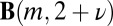is the beta function (27) and C is a normalization factor, such that the sum gives the total number of species. The tail of this distribution is described by the large m asymptotics of the beta function, which is a simple power function (the convergence to this asymptotic expression is very fast in the relevant parameter regime) (SI Appendix):

Some features of the process by Yule (3) and its corresponding SGD are noteworthy. First, as mentioned above, the Yule process is neutral (3), in the sense that the speciation rate is the same for all species and all times. Similarly, the chance of a new species to be the first member of a new genus is constant for any speciation event. Second, the distributions (Eq. 1 and expression 2) are not equilibrium distributions: as the number of species grows exponentially with time, so does, say, the number of genera with m species. However, if λ is the speciation rate, the actual number of species within a genus after a long time follows a deterministic behavior [i.e., ]. Therefore, n_m normalized by the total number of genera (which is the probability of having a genus of a specific size) is an equilibrium distribution.

The distribution suggested by Yule (3) [and other works that assumed strict power law statistics (25, 26)] generally fits observed data poorly, deviating meaningfully from the data (see below and SI Appendix for additional analyses), which can be seen in Fig. 1 for the SGD for the kingdom Animalia (11), and the best fit of the Yule function obtained by the least squares method.

Fig. 1.

The SGD statistics for the kingdom Animalia. The graph shows the number (n) of genera with m species on a double logarithmic scale (Pareto plot) with logarithmic binning (SI Appendix). The solid black line is the best fit of Yule’s model (Eq. 1) to the data, for which ν = 0.2 (3). This value was obtained by a least squares fit (distance has been measured in logarithmic units), where ν is a free parameter. The solid red line is the best fit of the SEO model (Eq. 4), with a diversification (speciation minus extinction) rate of γ = 0.063 ± 0.0032 and the probability of origination of a new genus (on speciation) of ν = 0.026 ± 0.001. The confidence intervals were obtained from a parametric bootstrap (more details in SI Appendix). A nonparametric bootstrap leads to confidence intervals about one-half the size. The slight deviations for m = 1 reflect the inadequacy of the continuous theory in this regime as explained in the text. Using Monte Carlo simulations, we can get estimates for the case m = 1 (Table 2). In the inset, we present the ratio between the observed statistics and the models’ predictions as a way to assess the models’ validity. A valid model should present a random distribution of the ratios around one, whereas an invalid model will present a trend. Yule (3) was aware of this problem and added two more parameters that improved the fit to the data, but these parameters obscured the underlying process. A discussion of this topic is in SI Appendix.

In Fig. 1, Inset, we present the ratio between the data and the fit of each point. Such a plot is needed to understand whether the deviations of the data from the model are caused by random noise (in which case the ratio should be distributed homogenously around one) or a systematic deviation between the model and the data (in which case there would be a trend of the ratio). The latter scenario, which is the case for the model by Yule (3), implies that the model describes the data poorly.

The problematic fit reflects the property of Yule’s expression (Eq. 1) that, for m > 2, the distribution quickly converges to the asymptotic power law (expression 2 and SI Appendix) (3). Thus, when plotted on a log–log scale, the SGD should decrease linearly as increases. Accordingly, the black line in Fig. 1 (which corresponds to Yule’s prediction) is quite straight on a log–log scale, as expected, and the bending at values of is almost invisible. In contrast, the actual data (blue circles), although linear for large m, exhibit a pronounced shoulder for small values of m, which is below the extrapolation of the large m straight line behavior.

Many empirical SGDs for different-sized taxa show the same type of bending at intermediate values of m (see below), which implies that Yule’s theory is incomplete. Some modern versions of Yule’s theory [like the version in the work by Scotland and Sanderson (28)] gave up the homogeneity assumption, but the resulting fits to empirical data suffer from similar problems.

Our aim here is to extend Yule’s model (3), while keeping its two main features: neutrality (all species have the same speciation rate and the same chance of forming a new genus on speciation) and homogeneity (rates are fixed in time). We suggest, in accord with the work by Patzkowsky (8), that Yule’s approach falls short, not because of its neutrality or homogeneity assumptions but rather, because it neglects extinction. In Yule’s model, the number of species is always growing, and existing species never go extinct. We will explain how extinction affects the qualitative features of the SGD statistics.

SEO Model

Although all species eventually go extinct, one might suppose that a speciation-only theory should work. Let us again assume speciation at rate λ and extinction at rate μ. As long as λ > μ (as suggested by the long-term average of branching rates estimated from available data) (29), the net diversification rate γ = λ − μ is positive. Given that γ determines the rate of increase in the number of species within a genus, the size of an extant genus has been growing on average. One can imagine that a speciation-only model with γ as the speciation rate might yield the same results as a model with both extinction and speciation but having the same net diversification rate γ. If, within 1 My, we have three speciation events and two extinctions on average, why can we not use a theory with one speciation per 1 My instead?

The answer has to do with the importance of fluctuations in this type of stochastic process, particularly in the presence of an absorbing state. Although the size of a genus increases on average, a given genus may also disappear because of random extinction events. After extinction, a genus cannot recover. Accordingly, the ratio between the numbers of genera in the larger genus size classes will satisfy the prediction of Yule’s theory (3), because with a positive diversification rate, they rarely go extinct; thus, the net growth rate approach works. For small genera, however, fluctuation-induced extinctions of a genus are relatively frequent, and one can notice a substantial underrepresentation of small genera with respect to the ratio suggested in Eq. 1. As can be seen in Fig. 1, the right tail of the distribution indeed follows a power law, but with respect to this power law, there is a pronounced underrepresentation of small genera that characterizes most SGDs.

The importance of extinction events and their role in shaping macroevolutionary patterns were already pointed out in the works by Aldous et al. (30, 31), which considered many features of the tree of life using a model that includes, as our model does, speciation, extinction, and origination of new genera. Aldous et al. (30, 31) assumed, however, that the overall diversification rate is zero, and therefore, on average, the number of lineages is kept fixed along the tree of life. The increase in the number of species with time appears only through the boundary conditions [i.e., Aldous et al. (30, 31) considered the set of γ = 0 processes conditioned on the number of species at present].

We suggest that the increase in the number of taxa through time is not a coincidence but that it reflects the fact that the diversification rate of extant clades has been positive. We also have to condition our process on the number of species at present, but the underlying dynamics are different; accordingly, the SGD has a totally different form. In particular, the real SGD statistics may admit a power law tail, and therefore, the chance of finding a huge genus is small but not negligibly small. As we shall show below, this result emerges naturally for γ > 0 processes, as is the case for most of the groups that we analyzed. In the model by Aldous et al. (30, 31) [also in a similar case considered recently by Foote (10)], the number of species within a genus is decreasing on average, because some of the speciation events lead to the origination of a new genus and do not contribute to the growth of the genus from which they emerged. For these models, there is a natural cutoff for the size of a genus, which is in contrast with most of the empirical datasets analyzed.

We assume that the current distribution of genus sizes within a clade (i.e., the existing species descending from a common ancestor) results from a neutral and homogenous stochastic process that includes speciation, extinction, and origination of new genera. In the SEO process, any species may produce an offspring lineage at rate λ or go extinct at rate μ, resulting in a diversification rate γ = λ − μ. In principle, the diversification rate may be either positive or negative, but clades with negative γ must disappear eventually. The rate may be defined with any unit of time, but the most natural unit is the average species lifetime. Accordingly, the extinction rate μ is fixed at one, and the speciation rate and genus origination rate are quantified as multiples of the extinction rate. Thus, although the SEO model is composed of three events, as a mathematical model of the SGD, it has only two free parameters—the diversification and origination rates.

On speciation, the newly emerging species may either be similar to its parent, in which case it will belong to the same genus, or differ substantially, thus becoming the first member of a new genus, with probability ν (0 < ν ≤ 1). Note that each of the new species can become a new genus, and thus, ν is a fraction of λ—the total rate of appearance of new species—and not γ, the net increase in number of species. Note that our model does not require that genera and other clades be monophyletic, because new genera can emerge from a branch of an existing genus, and it is likely that only young genera will be monophyletic. In one example that we analyzed below (32), we have observed this phenomenon.

The continuum approximation of the SEO process is given by the following equation (6, 7, 33) (SI Appendix has a description of the derivation):

where n(m) is the number of genera of size m. Here, (the number of species) and n(m) are regarded as continuous variables and not as integers, because the derivation of Eq. 3 neglects the discrete character of , following a standard procedure to describe a stochastic process by means of a Fokker–Plank equation (34). This approximation fails only for very small values, typically for m = 1 and m = 2 (35, 36). Accordingly, to compare the number of monotypes (m = 1) with the empirical data, we use numerical techniques as explained below.

The steady state solution of Eq. 3 takes two forms: one for γ > ν and one for γ < ν [both given in terms of the Kummer function ] (27). The qualitative difference between the two regimes is that, when species split more frequently than new genera originate, the number of species per genus increases on average. When the diversification rate is smaller than the genus origination rate, the size of a genus shrinks on average, and thus, one does not expect to find extremely large genera. When the system reaches a steady state, if γ > ν, the large asymptotic is a power law:

where , , and is the current population size (number of species observed today). For γ < ν, the SEO dynamics support a truncated power law distribution (i.e., the probability of very large genera is exponentially small; here, ):

In the following section, we will see that, for most of the empirically observed SGDs, it seems that the average growth rate of a genus is slightly larger than zero (i.e., that γ > ν). This finding is in contrast with the model suggested in the works by Chu and Adami (23) and Adami and Chu (24), where all taxa are extinction prone (i.e., the average number of daughter species that belong to the same genus is smaller than one). If this result were the case, one would expect an exponential cutoff of n(m) for large m, which is not the case for most of the taxonomic levels analyzed below.

Our model was previously introduced by Patzkowsky (8). However, he did not present an analytic solution, which we have just done, but limited model development to a recursion expression for the SGD that can be used to obtain a numerical solution. The advantage of analytic solutions is that they enable a general understanding of the shape of the SGD distribution for all cases and not just for those cases that were solved numerically. For example, only with the analytical solution can one observe that the two regimes present a qualitatively different behavior of the large genera (Eqs. 4 and 5).

Moreover, Patzkowsky (8) did not compare his model with SGD data, which we do below, but rather, he compared the average genus size as a function of time with paleontological data. Przeworski and Wall (9) applied the model by Patzkowsky to the SGD of real datasets but only used the size of the largest genus and the number of monotypes (i.e., genera of size one) rather than the whole distribution. This choice is problematic, because these two quantities are the noisiest parts of the SGD distribution and thus, do not permit a fine-tuned comparison of the model with the data. Therefore, Przeworski and Wall incorrectly claimed that the model cannot differentiate between dissimilar sets of parameters, believing that all sets of parameters will produce the same results. We show that the model can, indeed, differentiate between dissimilar sets of parameters, and thus, the speciation and origination rates can be inferred from the data. Because of what they perceived to be a limitation, Przeworski and Wall used a specific set of parameters to test different growth models (e.g., exponential growth vs. logistic growth) and concluded that exponential growth better described the observed monotypic and largest genus distributions, although arriving at this conclusion on the basis of a single set of parameters is questionable (9).

Reed and Hughes (37) suggested a similar model but assumed that the origination rate is homogeneous across genera, regardless of the number of species. This assumption seems doubtful, because new genera can originate from each of the species. Finally, Foote (10) recently used the model by Patzkowsky (8) to test whether two groups of mollusks had different rates of genus origination and showed that estimates of parameters for the two groups based on the SGD did, indeed, match rate estimates derived from paleontological data.

SEO Predictions.

The SGD statistics of the kingdom Animalia (11) are fit very well by Eq. 4 (Fig. 1, red solid line). The fitting was done by the least squares method, where we ascribe equal weight to small and large genera. The fit can be improved by taking into account the difference in the variance between small, medium, and large genera (the medium size has the smallest variance); however, we do not have a formula for the second moment, and thus, we assumed equal weights. The superiority of the SEO model over the Yule model (3) can be quantified in a few ways (more details in SI Appendix). First, the R² of the SEO model is 0.997, whereas it is 0.93 for Yule’s model. The relatively high R² of the Yule model should not be misleading, because such a smooth curve of the data is expected to have a high R². The F statistic test can measure the improvement in the SEO model over the Yule model, taking into account the fact that the SEO model has one additional free parameter. The P value of the difference between the two datasets is 1.5e-11, which is very low, showing that the improvement is real and not random.

Another measure of superiority of the SEO model over the Yule model is the (unsigned) area between the curve of the data and the curve of the fit (the lower the better). In the Yule model, it is 3.89, and in the SEO model, it is 0.024. A third measure is the ratio between the data and the fit for each of the two models (shown in Fig. 1, Inset). Whereas for the SEO model, the deviations are uniformly distributed around one, the Yule model exhibits a systematic deviation of the ratio (38). Such a trend shows that, even if the R² of the fit is close to unity, the model does not capture the true behavior of the data. In addition, the largest magnitude of the deviations for the Yule model is about 250%, whereas it is only 40% for the SEO model.

Fig. 2 presents a similar graph for the kingdom Plantae and the class Aves (binned with a fixed number of genera per bin) (SI Appendix). Again, the SEO model captures the entire dataset, including the small to intermediate m behavior.

Fig. 2.

SGD statistics for the kingdom Plantae (blue dots) and Aves class (open squares) compared with the fitted SEO model for (Upper Right Inset) the Plantae (diversification rate of γ = 0.055 ± 0.005 and origination probability of ν = 0.017 ± 0.0012) and (Lower Left Inset) the Aves (diversification rate of γ = 0.08 ± 0.021 and origination probability of ν = 0.089 ± 0.010).

The SGD is one prediction of the SEO model, with the advantage that a large amount of data of this type can be collected relatively easily, but other predictions of the SEO model that relate to the phylogenetic tree of species can be tested as well. For example, an assumption of the SEO model is that, on average, the size of a genus grows exponentially with its age, and thus, there should be a positive correlation between genus age and size. Another prediction is that the distribution of genus origination times (measured backward) should be left-skewed because of the fact that the number of new genera originating every generation is proportional to the number of species, which grows with time. It is difficult to collect data for these quantities, which would enable a precise fitting of the model to the data. However, it is still possible to test the general behavior of the limited available data for a basic qualitative agreement between the model’s predictions and the data.

The sizes of taxonomic groups and their ages have been shown to be positively correlated in some analyses (39, 40) and unrelated in others (41). However, for our purposes, it is important to test the relationship between age and diversity at the low level of genera. As far as we know, no wide-scale analysis of such a relationship has been undertaken, and conducting such an analysis is outside the scope of this article. However, we analyzed the genera of one family to test the age skewedness, and in that context, we also analyzed the age–diversity correlation.

To this end, we used the phylogenetic tree of the Furnariidae family of suboscine passerine birds constructed by Derryberry et al. (32). We chose this family, because it is a relatively large group with an existing phylogenetic tree of virtually all species. Using this tree, we obtained the crown age of each genus (the age of the most recent common ancestor of all of the species; see below) and its size. Fig. 3 presents the size of each genus vs. its age (not including monotypes because of the inability to determine their age). Although the process is noisy, the growth of the genus size with age is still clearly seen (the data for Fig. 3 are given in SI Appendix, Table S2), and the slope of size vs. age is 0.099 (0–0.2) per species generation, which is similar to the exponential growth rate of the number of species of passerine birds.

Fig. 3.

The correlation between the age of a genus and its size is presented. The x axis is the crown age of a genus as estimated in the work by Derryberry et al. (32). The y axis is the log (base e) of the size of the genus. The red line is the linear fit of the data that corresponds to exponential growth. The result is consistent with the SEO model that predicts an exponential growth. The slope of the linear fit is 0.047 (0–0.095) per million years. Assuming a species generation time of 2.1 My, the slope is 0.099 (0–0.2), which is similar to the result that we get below for the passerine birds.

Furthermore, as expected from the SEO model, the skew of the ages of the 38 genera in the Furnariidae family is indeed positive: 1.95 (which is about five times larger than the SE of the skew at 0.4; i.e., P < 10e-6). This strong bias can also be seen in Fig. 3. To test whether this strength of skew is expected under the SEO model, we simulated 1,000 realizations with the parameters of the Furnariidae family: n = 247, λ = 0.10, and ν = 0.12. The age skew of genera within the Furnariidae was inside the 95% confidence interval of the simulations. Finer measures, like the mode, are harder to estimate given the small number of genera.

Inference from the SEO Model.

The fit of the SEO model to an observed SGD generates estimates of past demographic parameters. These parameters may be compared with estimates from other methods to assess the realism of the SEO model. For example, in Fig. 2, we consider genera within the class Aves. The fitted value for the average rate of diversification can be used to estimate the time of origin of birds, which is consistent with estimates based on paleontological and molecular data.

It should be noted that, in the framework of the SEO model, the time of origin of a taxonomic group is the time when the first species of this group appeared. This time may be older than both the crown age (the age of the most recent common ancestor of all existing species) and the age of the oldest fossil. Nevertheless, estimates of the origination times of major taxa have sufficient uncertainty that we would not expect more than a general correspondence to estimates derived from the SEO model.

With a fixed exponential growth rate, we can estimate the time of the most recent common ancestor of modern birds from the total number of bird species (N) and the diversification rate, which would be T = ln(N)/γ = 114 (97–138) generations ago. Assuming that a generation (a species duration) is between 1.4 and 2.8 My (42), we derive T = 239 My (95% confidence interval = 386–135; we multiply the expectation by 2.1 My, the lower boundary by 1.4 My, and the upper boundary by 2.8 My), which brackets the earliest appearance of avian ancestors in the fossil record (43). When species can become extinct, an unbiased estimate of T can be obtained by accounting explicitly for the rates of speciation (λ = γ + 1) and extinction (μ = 1 in this analysis). The equation describing this process (42) is n = (λ·exp[γt] − 1)/γ, which can be rewritten as T = ln([γN + 1]/λ)/γ . In this case, λ = 1.08, μ = 1, n = 9,913, and t = 82.5 species lifespans, which translates into 172 My assuming a generation time of 2.1 My.

Estimates of the times of origin based on the SEO model fits for other classes of plants and animals based on ref. 42 show a similar reasonable correspondence (Table 1). It is important to emphasize that our model’s time unit is the abstract quantity of generation time (i.e., the typical time until the extinction of a species for each group). This quantity may vary substantially between taxonomic groups. For example, the life expectancy of individuals will affect the extinction rate of the species. Thus, we could not easily convert generation units to millions of years, which needs to be done to allow a comparison with estimates from other sources. Because the generation time of passerine birds has been estimated, we simply took this number and applied it to all of the taxonomic groups to allow a conversion to millions of years, although this translation is, of course, imprecise. Accordingly, we only expect a general correspondence comparing our method’s results with estimates from other sources.

Table 1.

Diversification rate and the appearance time for different classes

Name	Size (no. of species)	Diversification rate γ (± SD) and origination rate ν (± SD)	Generations since origination	Estimated time to origination T (My)	Independent estimate of T (My)
Arachnida	55,147	γ = 0.055 ± 0.0064	144 (131–161)	302 (183–450)	420
		ν = 0.0359 ± 0.0023
Magnoliopsida (Angiospermopsida)	87,281	γ = 0.051 ± 0.0058	163 (148–182)	342 (207–509)	228
		ν = 0.015 ± 0.0012
Insecta	661,370	γ = 0.037 ± 0.0019	272 (260–285)	571 (364–798)	420
		ν = 0.0185 ± 0.0006
Diplopoda	9,907	γ = 0.23 ± 0.0348	32 (28–37)	67 (39–103)	420
		ν = 0.10 ± 0.012
Aves	9,913	γ = 0.08 ± 0.021	82 (67–107)	172 (93–299)	130
		ν = 0.089 ± 0.010
Passerine birds (order)	6,198	γ = 0.12 ± 0.015	54 (48–60)	113 (67–168)	82
		ν = 0.14 ± 0.013
Malacostraca	18,419	γ = 0.086 ± 0.0115	84 (76–95)	176 (106–266)	510
		ν = 0.068 ± 0.0054
Maxillopoda	4,963	γ = 0.06 ± 0.0096	94 (83–108)	197 (116–302)	500
		ν = 0.074 ± 0.0146
Amphibia	5,753	γ = 0.051 ± 0.0118	110 (93–137)	231 (130–383)	315
		ν = 0.032 ± 0.0042
Mammalia	4,832	γ = 0.15 ± 0.0176	42 (39–47)	88 (54–131)	120
		ν = 0.118 ± 0.019

The SGD of each class has been fitted (Fig. 2 shows an example) using the SEO model to yield the diversification rate γ (column 3). From the total number of species in the class (column 2) and the diversification rate, one may extract the number of generations since the first appearance of this class (column 4). To translate generations to time, we took a single generation (typical time to extinction) as 2.1 (1.4–2.8) My as presented in column 5. This result of the SEO model should be compared with other independent estimates based on either fossil data or genetic analysis (column 6). In most cases, the SEO-based estimates are close to the results from independent sources. Note that the definition of generation time is quite arbitrary and may vary among classes, which may explain some mismatch with the fossil data. The factor-of-two differences for Malacostraca and Maxillopoda may be related to incomplete data about the number of species. For Diplopoda, the estimates are inconsistent; they may reflect an inadequacy of our demographic model in this case or an underestimation for the generation time of diplopod species. The Mammal class is dominated by the placentals (4,600 of 4,832 species), and therefore, the appropriate time is given for the placentals. The references to independent estimates of T are given in SI Appendix, Table S3.

In some of the cases, there is a surprisingly good match between our estimates and molecular or fossil estimates for the origination time. Other than the estimate for Diplopoda, which is substantially off, all of the others differ at most by a factor of two from molecular and fossil estimates, which is notable given the imprecise conversion method described above, and it further supports the model’s plausibility.

An interesting point emerging from Table 1 is that the diversification rates are low relative to the rate of extinction. The diversification rate γ is based on a generation timescale (i.e., μ = 1). Thus, λ (the speciation rate) is simply 1 + γ on the same timescale, and the ratio of extinction to speciation is 1/(1 + γ). Because γ tends to be relatively low (Table 1, 0.04–0.23), the ratio of extinction to speciation is high (ca. 80–95%), which is what one would expect if the number of species in some of these taxa has been more or less steady over long periods.

Other predictions of the SEO model can be compared with the observed data, particularly the number of monotypic genera and the relative size of the largest genus, which was attempted in refs. 9 and 28. These values are estimated from the fitted values of γ and ν for several large classes of animals and plants and compared with observed data in Table 2. Because the SEO continuum limit does not hold for genera of size one, we obtained predicted numbers of monotypic genera using simulations of 1,000 replicates of the SEO process with the estimated parameters and observed number of species (a detailed description of the simulation procedure as well as an explanation of the special treatment of the largest genus is in SI Appendix). The confidence intervals were obtained from the SD of these simulations. One can see that, in general, the expectations of the model for both the number of monotypes and the size of the dominant genus are of the order of the real data.

Table 2.

The observed number of monotypic genera and the number of species in the largest genus for different classes of animals and plants

Class	Monotypes		Dominant
	Data	Model	Data	Model
Arachnida	1,752	2,060 ± 50	638	880 ± 370
Magnoliopsida (Angiospermopsida)	1,630	1,350 ± 38	6,606	9,885 ± 3,900
Insecta	19,477	13,580 ± 150	3,549	8,749 ± 3,900
Diplopoda	1,222	1,070 ± 53	325	515 ± 240
Aves	887	930 ± 35	80	120 ± 35
Malacostraca	1,326	1,320 ± 43	291	300 ± 115
Maxillopoda	396	360 ± 20	67	120 ± 37
Amphibia	129	170 ± 15	704	390 ± 170
Mammalia	525	705 ± 30	172	85 ± 30

These numbers are compared with the predictions of the SEO theory given the parameters γ and ν retrieved from the best fits of the SGD curve. The errors given reflect 1 SD about the mean of the simulated values.

We additionally compared the growth rate of the Aves class predicted by our model with the rate deduced from the phylogenetic tree of the suboscine passerine birds in South America (44): γ = 0.07–0.14 per My. Translating our prediction from generations to millions of years, we get γ = 0.0571 [0.0964–0.0375; assuming a mean generation of 2.1 My (1.4 My for the high diversification rate and 2.8 My for the low diversification rate)]. Thus, the estimates are similar. We furthermore compared the origination rate of genera of the class Aves (given in Table 1) with the origination rate that we derived from the phylogenetic tree of the Furnariidae family of the Aves class (38) (details for this derivation are in SI Appendix). The estimated ν-value for the Furnariidae family is 0.096 (0.038–0.3) per speciation event [assuming a generation time of 2.1 My for the mean (1.4 My for the lower bound and 2.8 My for the upper bound)], which is similar to the value of the Aves class generally from the SEO model (0.08 ± 0.021).

Model Differentiation.

Both the Yule (3) and SEO models assume that the overall number of species grows exponentially and that the diversification rate is homogenous in time. This assumption contradicts a common understanding in the field, namely that the number of species within a taxon initially grows exponentially (the adaptive radiation phase) and then levels off when ecological space has been filled (21, 45–51). In the latter saturation phase, turnover of species may occur, but on average, the number of extinctions balances the number of species origination events.

When one assumes a model and infers parameters by fitting the model to data, one will always produce estimates for the model, regardless of whether the model fits the data well. Accordingly, it is important to test the performance of a model against data that result from processes that violate the assumptions of the model. Therefore, we estimated SEO models for SGDs produced by numerical simulations from alternative processes, particularly the imposition of an upper limit to clade size after a period of exponential growth.

Fig. 4 sets the framework for the discussion below. It shows the log of the number of species vs. time in two different scenarios: (i) initial, almost exponential growth (more precisely, it has not been bounded yet) and (ii) constrained growth (in this case, modeled as a logistic equation):

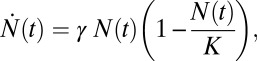where is the number of species, γ is the initial diversification rate, and is the maximal number of species in the taxonomic group, which reflects, roughly, the number of different ecological niches. Early in the diversification of a clade (stage 1), exponential and logistic processes are almost identical, because the finite carrying capacity of the logistic model has little effect at low densities. In stage 2, the growth rate of the number of species in the logistic system starts declining, and in stage 3, it approaches zero. Note that stage 3 is a special case of an unbounded exponential growth with .

Fig. 4.

Semilog (number of species) vs. time for unbounded (red) and constrained (blue) growth. During stage 1 (), both constrained and unconstrained systems increase exponentially. During stage 3 (), the system is no longer growing (). After a period, the system will attain SEO steady state during both stages. Only during the transitional stage 2 will the system deviate significantly from the predictions of the SEO model.

The difference between the two growth patterns should manifest itself in the intermediate stage (2), where approaches and the growth rate is slowing rapidly. Under this circumstance, the SEO assumption of a fixed diversification rate is not valid, and Eq. 4 should not be an accurate description of the system in that stage.

Examples for the SGDs of each of the stages are presented in Figs. 5, 6, and 7. Here, the results of simulations of a logistic growth process () are compared with the best fit to the unbounded growth formula in Eqs. 4 and 5 (if , clearly ). During the first and third stages, the inference works well; the SGDs are fitted closely, and the underlying parameters of the model are recovered. In contrast, for the statistics collected during the second stage, the deviations are large (up to 100%) (Fig. 7, Inset) and exhibit a systematic trend. Thus, it is clear that, during this stage, the SEO process fails to fit the data. Because the distribution evolves with time according to Eq. 3, it takes some time for the SGD to reflect the reduced growth rate as the number of genera approaches the asymptote. For this reason, the SGD that corresponds to a particular stage appears after some time lag after the onset of that stage. For example, the second stage distribution shown in Fig. 6 was measured 30 generations after saturation [saturation is defined, quite arbitrarily, at N(t) = 0.95K]; that amount of time was insufficient to attain a zero growth SGD, which became established more than 100 generations after saturation (Fig. 6). In contrast to this behavior, the convergence to the steady state of exponential diversifications when starting from a single species is relatively short—only a few generations.

Fig. 5.

The SGD of a logistic growth process during its first (exponential) stage. The SGD statistics were collected from the simulation when the number of species had reached (i.e., one-tenth of the carrying capacity K). The red line corresponds to Eq. 4 with the best fit parameters and , which closely approximate the underlying values of the simulated process. In the inset, we present the ratio between the observed statistics and the model's predictions, as was done in the inset of Fig. 1.

Fig. 6.

Same as Fig. 5 for stage 3. Here, the system was sampled 100 generations after saturation had been reached. The inferred parameters are γ = 0.001 (very close to zero) and ν = 0.039. Note that ν > γ, and therefore, Eq. 5 was used to fit the simulated data. In the inset, we present the ratio between the observed statistics and the model's predictions, as was done in the inset of Fig. 1.

Fig. 7.

Same as Fig. 5 for stage 2. The system was sampled 30 generations after saturation [i.e., after N(t) is more than 95% of K, the carrying capacity of the logistic process] before reaching the equilibrium. Instead, the fit yields and . The inset shows the systematic deviations of the fit/data ratio and indicates the inadequacy of the model in this case.

The goodness of fit that we illustrated schematically before can be quantified by using the sum of squared deviations (SS) between the data and the theory. For each of the three stages that we fitted, we simulated 1,000 replicates under the assumption of pure exponential growth with the parameters of the best fit. We fitted these new replicates to the SEO model and determined the SS of each of the 1,000 replicates. This procedure gives us the distribution of the SS for each of the stages. By comparing the SS obtained for the logistic growth with the distribution of the SS, we can estimate how likely it is to obtain such deviations. As expected for stages 1 and 3, the SS was smaller than 95% of the replicates, whereas for stage 2, the SS was larger than 95% of them. Thus, our model cannot accurately describe the logistic growth in the transition phase.

A similar test was done for a model where, instead of a logistic growth, the growth rate declines like a power law g = g₀/t^α as in ref. 21. In this model, the SS in all of the cases was similar to the SS obtained from a pure exponential growth. This result implies that our model is sensitive only to large deviations from the models’ assumption, whereas more subtle deviations cannot be detected.

We tested the SEO model for all taxonomic groups of the rank of order and higher that have at least 500 species and 100 genera. From 151 such groups, the SEO model was not rejected for 130 of them, which is more than expected at random. These data are presented in SI Appendix. It is important to emphasize that the fact that the sum of squared deviations is smaller than 95% of the SEO cases does not tell us what is the true model describing the data, because it could be exponential growth but also another similar growth model.

Thus far in this section, we analyzed the sensitivity of our model to changes in its assumption of time homogeneity. Another aspect of applying a model to a system is to test its robustness to changes in its assumptions. Both aspects are important, because although we want our model to be sensitive to meaningful deviations from its assumptions, we do not want it to be sensitive to minor deviations. Finally, we test the robustness of our model to such minor deviations by using data produced from a population with a nonhomogeneous diversification rate and testing whether we can determine its parameter averages by fitting the SEO model.

Sensitivity of the SEO Model.

It is highly improbable that the rates of diversification and origination should be homogeneous over time, and therefore, the SEO model is plausible only if its results are robust against weak perturbations. Accordingly, we repeated the simulation of the evolutionary process three times with the following different types of randomness in the parameters: (i) the diversification rate jumps, at random times, between low and high values (dichotomous noise); (ii) at each time step, the rates γ and ν are picked at random from a normal distribution (Gaussian noise); and (iii) at each time step, the rates are picked at random from an exponential distribution (exponential noise). As expected, the emergent SGD distributions are noisier, but the inferred parameters are, in all three cases, more or less the time averages of the diversification and the origination rates. The exact procedure used to obtain these results is given in SI Appendix.

Noise in the origination rate can also be caused by the alternate classifications of different taxonomists. The fact that noise in the origination rate does not eliminate the ability to infer on average, the growth rate and the diversification rate but rather, enlarges the error range, shows that our model is robust to the subjectivity of the classification process.

Discussion

The SEO model presented here can describe observed SGD distributions of higher taxonomic groups, and it thereby constitutes an interesting null alternative in the negative sense, which we explained in the Introduction. We have also attempted to establish the SEO model as a plausible description of the real macroevolutionary process. If it is, the fit of the model parameters to the observed SGD would allow one to infer both the diversification rate γ and the probability of origination of a new genus per speciation event ν. The origination parameter ν, thus, represents the probability that a new species (i.e., producing the contemporary descendants of a new evolutionary lineage) is phenotypically sufficiently distinct to be given a new generic epithet.

As mentioned, although the model had been previously described and applied in a limited fashion, we have undertaken a wide-scale analysis of SGDs across many taxonomic groups. Furthermore, we compared multiple predictions of the model with estimates based on other sources to establish the model’s realism. We further tested the robustness of the model to identify which taxonomic groups it can describe. An interesting conclusion that we deduced is the low diversification rate of almost all of the taxonomic groups tested, consistent with a high turnover rate of species, which was not evident in previous works (17, 52, 53).

Our model assumes both an exponential growth and an origination rate that are constant in time and also uniform among different genera. These homogenous assumptions have been shown to be invalid for most groups tested (54). In addition, we assumed that there is no limit to the exponential growth, which obviously cannot be sustained forever.

Regarding the lack of a limit, a more reasonable model is one of adaptive radiation, where after a growth period, the number of species plateaus. Such a limit to species richness is probably the case for lower taxonomic levels, where the SGD distributions do not always follow our SEO model (e.g., the SGD of the Nymphalidae family in SI Appendix, Fig. S8), which probably reflects the decrease in the diversification rate as the number of species approaches saturation. In addition, in some cases, the estimated growth rates are extremely small, reflecting that the system is already in the saturation region (more details in SI Appendix). However, at higher taxonomic levels, exponential growth might continue, because even if one family saturates, others may continue growing; therefore, new families may emerge, creating growth of the clade as a whole. Thus, our model, which assumes exponential growth, can describe the behavior of the species dynamic of high taxonomic groups that are not yet in a saturation regime. Regarding constant growth rates, although, for example, a constant diversification rate through time is clearly unrealistic, the SEO model can still be plausible as an estimation of the average diversification at the broad class level. Furthermore, as we showed, our model can discriminate only between models that are substantially different from the pure exponential growth, such as a logistic model that is in the transition between the exponential growth and saturation phases. Models that do not differ significantly, such as a gradual decline in the diversification rate or randomness in the diversification rate, cannot be ruled out by the SGD data. Thus, the SEO model at a minimum has value in its ability to discriminate between substantially different models of growth.

An interesting direction to extend the SEO model would be to develop a multihierarchy model that combines the origination, speciation, and extinction of higher taxonomic levels. For example, it may include species, genera, and families simultaneously. A more limited extended model would describe the dynamics of species within families or genera within families, etc. Although such an extension is worth pursuing, its success cannot be taken for granted based on the success of the SEO model for the SGD. Phyla, for example, clearly do not follow such a model, because the time of the appearance of almost all of them is similar. Such an extension deserves its own treatment in another work.

Rather than deal with the mean number of genera of a given size, another interesting direction to extend the model would be to obtain a full probability function for the species distribution (i.e., what is the probability of having a specific combination of genus sizes; e.g., n₁ = 103, n₂ = 91, n₃ = 74, etc.). Such a formula was obtained by Ewens (55) for the special case of a fixed population. Such a function can be used to obtain estimates by the maximum likelihood approach instead of a simple fitting. The maximum likelihood approach can take into account more information than the continuum approximation of the mean that we used here. Also, it may enable us to obtain estimates when using smaller numbers of species. However, obtaining the full probability function is not simple, and even calculating it numerically or estimating it by simulations requires careful work that is beyond the scope of the present analysis.

In closing, we have shown that a simplified model of species evolution can explain the global features of the SGD within large taxonomic groups relatively accurately as well as some other features. This result suggests that complicated processes related to interactions between species, including niche saturation, and environmental effects average out when dealing with phylum- and class-level taxa; therefore, they can be neglected for a first approximation. Moreover, the fact that model parameters describing SGDs of several classes correspond well to the appearance times of the classes suggests that, although the classification of species and even more so, genera are manmade constructs, the SEO model fairly accurately reflects the real evolutionary process.

References

- 1.Raup D. Extinction: Bad genes or bad luck? New Sci. 1991;131(1786):46–49. [PubMed] [Google Scholar]
- 2.Raup DM, Gould SJ, Schopf TJM, Simberloff DS. Stochastic models of phylogeny and evolution of diversity. J Geol. 1973;81(5):525–542. [Google Scholar]
- 3.Yule GU. A mathematical theory of evolution, based on the conclusions of Dr. JC Willis, FRS. Philos Trans R Soc Lond B Biol Sci. 1925;213:21–87. [Google Scholar]
- 4.Hubbell SP. The Unified Neutral Theory of Biodiversity and Biogeography. Princeton: Princeton Univ Press; 2001. [DOI] [PubMed] [Google Scholar]
- 5.Volkov I, Banavar JR, Hubbell SP, Maritan A. Neutral theory and relative species abundance in ecology. Nature. 2003;424(6952):1035–1037. doi: 10.1038/nature01883. [DOI] [PubMed] [Google Scholar]
- 6.Maruvka YE, Shnerb NM, Kessler DA. Universal features of surname distribution in a subsample of a growing population. J Theor Biol. 2010;262(2):245–256. doi: 10.1016/j.jtbi.2009.09.022. [DOI] [PubMed] [Google Scholar]
- 7.Manrubia SC, Zanette DH. At the boundary between biological and cultural evolution: The origin of surname distributions. J Theor Biol. 2002;216(4):461–477. doi: 10.1006/jtbi.2002.3002. [DOI] [PubMed] [Google Scholar]
- 8.Patzkowsky ME. A hierarchical branching model of evolutionary radiations. Paleobiology. 1995;21(4):440–460. [Google Scholar]
- 9.Przeworski M, Wall JD. An evaluation of a hierarchical branching process as a model for species diversification. Paleobiology. 1998;24(4):498–511. [Google Scholar]
- 10.Foote M. Evolutionary dynamics of taxonomic structure. Biol Lett. 2012;8(1):135–138. doi: 10.1098/rsbl.2011.0521. [DOI] [PMC free article] [PubMed] [Google Scholar]
- 11.Bisby FA, et al. Species 2000 & ITIS Catalogue of Life. Reading, United Kingdom: Univ of Reading; 2010. [Google Scholar]
- 12.Jablonski D, Finarelli JA. Congruence of morphologically-defined genera with molecular phylogenies. Proc Natl Acad Sci USA. 2009;106(20):8262–8266. doi: 10.1073/pnas.0902973106. [DOI] [PMC free article] [PubMed] [Google Scholar]
- 13.Collar DC, Near TJ, Wainwright PC. Comparative analysis of morphological diversity: Does disparity accumulate at the same rate in two lineages of centrarchid fishes? Evolution. 2005;59(8):1783–1794. [PubMed] [Google Scholar]
- 14.Pyron RA, Burbrink FT. Trait-dependent diversification and the impact of palaeontological data on evolutionary hypothesis testing in New World ratsnakes (tribe Lampropeltini) J Evol Biol. 2012;25(3):497–508. doi: 10.1111/j.1420-9101.2011.02440.x. [DOI] [PubMed] [Google Scholar]
- 15.Rabosky DL. Positive correlation between diversification rates and phenotypic evolvability can mimic punctuated equilibrium on molecular phylogenies. Evolution. 2012;66(8):2622–2627. doi: 10.1111/j.1558-5646.2012.01631.x. [DOI] [PubMed] [Google Scholar]
- 16.Harmon LJ, et al. Early bursts of body size and shape evolution are rare in comparative data. Evolution. 2010;64(8):2385–2396. doi: 10.1111/j.1558-5646.2010.01025.x. [DOI] [PubMed] [Google Scholar]
- 17.Stadler T. Mammalian phylogeny reveals recent diversification rate shifts. Proc Natl Acad Sci USA. 2011;108(15):6187–6192. doi: 10.1073/pnas.1016876108. [DOI] [PMC free article] [PubMed] [Google Scholar]
- 18.Aldous DJ. Stochastic models and descriptive statistics for phylogenetic trees, from Yule to today. Stat Sci. 2001;16(1):23–34. [Google Scholar]
- 19.Nee S. Birth-death models in macroevolution. Annu Rev Ecol Evol Syst. 2006;37:1–17. [Google Scholar]
- 20.Cardillo M, Huxtable JS, Bromham L. Geographic range size, life history and rates of diversification in Australian mammals. J Evol Biol. 2003;16(2):282–288. doi: 10.1046/j.1420-9101.2003.00513.x. [DOI] [PubMed] [Google Scholar]
- 21.Nee S, Mooers AO, Harvey PH. Tempo and mode of evolution revealed from molecular phylogenies. Proc Natl Acad Sci USA. 1992;89(17):8322–8326. doi: 10.1073/pnas.89.17.8322. [DOI] [PMC free article] [PubMed] [Google Scholar]
- 22.MacArthur RH. On the relative abundance of bird species. Proc Natl Acad Sci USA. 1957;43(3):293–295. doi: 10.1073/pnas.43.3.293. [DOI] [PMC free article] [PubMed] [Google Scholar]
- 23.Chu JH, Adami C. A simple explanation for taxon abundance patterns. Proc Natl Acad Sci USA. 1999;96(26):15017–15019. doi: 10.1073/pnas.96.26.15017. [DOI] [PMC free article] [PubMed] [Google Scholar]
- 24.Adami C, Chu JH. Critical and near-critical branching processes. Phys Rev E Stat Nonlin Soft Matter Phys. 2002;66(1 Pt 1):011907. doi: 10.1103/PhysRevE.66.011907. [DOI] [PubMed] [Google Scholar]
- 25.Burlando B. The fractal geometry of evolution. J Theor Biol. 1993;163(2):161–172. doi: 10.1006/jtbi.1993.1114. [DOI] [PubMed] [Google Scholar]
- 26.Burlando B. The fractal dimension of taxonomic systems. J Theor Biol. 1990;146(1):99–114. [Google Scholar]
- 27.Abramowitz M, Stegun I. Handbook of Mathematical Functions. Washington, DC: Government Printing Office; 1972. [Google Scholar]
- 28.Scotland RW, Sanderson MJ. The significance of few versus many in the tree of life. Science. 2004;303(5658):643. doi: 10.1126/science.1091483. [DOI] [PubMed] [Google Scholar]
- 29.Gilinsky NL. The pace of taxonomic evolution. In: Gilinsky NL, Signor PW, editors. Analytical Paleobiology. Short Courses in Paleontology. Vol 4. Knoxville, TN: Paleontological Society; 1991. pp. 157–174. [Google Scholar]
- 30.Aldous D, Krikun M, Popovic L. Stochastic models for phylogenetic trees on higher-order taxa. J Math Biol. 2008;56(4):525–557. doi: 10.1007/s00285-007-0128-0. [DOI] [PubMed] [Google Scholar]
- 31.Aldous DJ, Krikun MA, Popovic L. Five statistical questions about the tree of life. Syst Biol. 2011;60(3):318–328. doi: 10.1093/sysbio/syr008. [DOI] [PubMed] [Google Scholar]
- 32.Derryberry EP, et al. Lineage diversification and morphological evolution in a large-scale continental radiation: The neotropical ovenbirds and woodcreepers (aves: Furnariidae) Evolution. 2011;65(10):2973–2986. doi: 10.1111/j.1558-5646.2011.01374.x. [DOI] [PubMed] [Google Scholar]
- 33.Maruvka YE, Kessler DA, Shnerb NM. The birth-death-mutation process: A new paradigm for fat tailed distributions. PLoS One. 2011;6(11):e26480. doi: 10.1371/journal.pone.0026480. [DOI] [PMC free article] [PubMed] [Google Scholar]
- 34.Van Kampen NG. Stochastic Processes in Physics and Chemistry. Amsterdam: North-Holland; 1981. [Google Scholar]
- 35.Kessler DA, Shnerb NM. Extinction rates for fluctuation-induced metastabilities: A real-space WKB approach. J Stat Phys. 2007;127(5):861–886. [Google Scholar]
- 36.Ovaskainen O, Meerson B. Stochastic models of population extinction. Trends Ecol Evol. 2010;25(11):643–652. doi: 10.1016/j.tree.2010.07.009. [DOI] [PubMed] [Google Scholar]
- 37.Reed WJ, Hughes BD. On the size distribution of live genera. J Theor Biol. 2002;217(1):125–135. doi: 10.1006/jtbi.2002.3009. [DOI] [PubMed] [Google Scholar]
- 38.Press WH, Flannery BP, Teukolsky SA, Vetterling WT. Numerical Recipes. Cambridge, United Kingdom: Cambridge Univ Press; 1986. [Google Scholar]
- 39.McPeek MA, Brown JM. Clade age and not diversification rate explains species richness among animal taxa. Am Nat. 2007;169(4):E97–E106. doi: 10.1086/512135. [DOI] [PubMed] [Google Scholar]
- 40.Meredith RW, et al. Impacts of the Cretaceous Terrestrial Revolution and KPg extinction on mammal diversification. Science. 2011;334(6055):521–524. doi: 10.1126/science.1211028. [DOI] [PubMed] [Google Scholar]
- 41.Rabosky DL, Slater GJ, Alfaro ME. Clade age and species richness are decoupled across the eukaryotic tree of life. PLoS Biol. 2012;10(8):e1001381. doi: 10.1371/journal.pbio.1001381. [DOI] [PMC free article] [PubMed] [Google Scholar]
- 42.Ricklefs RE. Estimating diversification rates from phylogenetic information. Trends Ecol Evol. 2007;22(11):601–610. doi: 10.1016/j.tree.2007.06.013. [DOI] [PubMed] [Google Scholar]
- 43.Padian K, Chiappe LM. The origin and early evolution of birds. Biol Rev Camb Philos Soc. 1998;73(1):1–42. [Google Scholar]
- 44.Ricklefs RE. The unified neutral theory of biodiversity: Do the numbers add up? Ecology. 2006;87(6):1424–1431. doi: 10.1890/0012-9658(2006)87[1424:tuntob]2.0.co;2. [DOI] [PubMed] [Google Scholar]
- 45.Sepkoski JJ, Hulver ML. An atlas of Phanerozoic clade diversity diagrams. In: Valentine JW, editor. Phanerozoic Diversity Patterns: Profiles in Macroevolution. Princeton: Princeton Univ Press; 1985. pp. 11–39. [Google Scholar]
- 46.Benton MJ. Models for the diversification of life. Trends Ecol Evol. 1997;12(12):490–495. doi: 10.1016/s0169-5347(97)84410-2. [DOI] [PubMed] [Google Scholar]
- 47.Rabosky DL, Lovette IJ. Density-dependent diversification in North American wood warblers. Proc Biol Sci. 2008;275(1649):2363–2371. doi: 10.1098/rspb.2008.0630. [DOI] [PMC free article] [PubMed] [Google Scholar]
- 48.Rabosky DL. Ecological limits and diversification rate: Alternative paradigms to explain the variation in species richness among clades and regions. Ecol Lett. 2009;12(8):735–743. doi: 10.1111/j.1461-0248.2009.01333.x. [DOI] [PubMed] [Google Scholar]
- 49.Rabosky DL, Glor RE. Equilibrium speciation dynamics in a model adaptive radiation of island lizards. Proc Natl Acad Sci USA. 2010;107(51):22178–22183. doi: 10.1073/pnas.1007606107. [DOI] [PMC free article] [PubMed] [Google Scholar]
- 50.Ricklefs RE. Evolutionary diversification, coevolution between populations and their antagonists, and the filling of niche space. Proc Natl Acad Sci USA. 2010;107(4):1265–1272. doi: 10.1073/pnas.0913626107. [DOI] [PMC free article] [PubMed] [Google Scholar]
- 51.Ricklefs RE, Schluter D, editors. Species Diversity in Ecological Communities: Historical and Geographical Perspectives. Chicago: Univ of Chicago Press; 1993. [Google Scholar]
- 52.Rabosky DL, Lovette IJ. Explosive evolutionary radiations: Decreasing speciation or increasing extinction through time? Evolution. 2008;62(8):1866–1875. doi: 10.1111/j.1558-5646.2008.00409.x. [DOI] [PubMed] [Google Scholar]
- 53.Rabosky DL. Extinction rates should not be estimated from molecular phylogenies. Evolution. 2010;64(6):1816–1824. doi: 10.1111/j.1558-5646.2009.00926.x. [DOI] [PubMed] [Google Scholar]
- 54.Morlon H, Potts MD, Plotkin JB. Inferring the dynamics of diversification: A coalescent approach. PLoS Biol. 2010;8(9):13. doi: 10.1371/journal.pbio.1000493. [DOI] [PMC free article] [PubMed] [Google Scholar]
- 55.Ewens WJ. The sampling theory of selectively neutral alleles. Theor Popul Biol. 1972;3(1):87–112. doi: 10.1016/0040-5809(72)90035-4. [DOI] [PubMed] [Google Scholar]
Associated Data
This section collects any data citations, data availability statements, or supplementary materials included in this article.