Molecular mechanisms of multiple toxin–antitoxin systems are coordinated to govern the persister phenotype

Significance

Persisters are drug-tolerant bacteria that account for the majority of bacterial infections. They are not mutants, but rather slowly growing cells in a heterogeneous population. Evidence links them to the toxin–antitoxin systems present in nearly all bacteria. To explore the connection, we have created a system-level model of toxin–antitoxin systems that includes molecular mechanisms, stochastic fluctuations, variable growth rate, and population dynamics. The results quantitatively describe how a noisy environment can give rise to a bet-hedging subpopulation of persisters that always exists, not just in reaction to stress. Furthermore, multiple toxin–antitoxin systems can cooperate to increase the persister frequency.

Abstract

Toxin–antitoxin systems are ubiquitous and have been implicated in persistence, the multidrug tolerance of bacteria, biofilms, and, by extension, most chronic infections. However, their purpose, apparent redundancy, and coordination remain topics of debate. Our model relates molecular mechanisms to population dynamics for a large class of toxin–antitoxin systems and suggests answers to several of the open questions. The generic architecture of toxin–antitoxin systems provides the potential for bistability, and even when the systems do not exhibit bistability alone, they can be coupled to create a strongly bistable, hysteretic switch between normal and toxic states. Stochastic fluctuations can spontaneously switch the system to the toxic state, creating a heterogeneous population of growing and nongrowing cells, or persisters, that exist under normal conditions, rather than as an induced response. Multiple toxin–antitoxin systems can be cooperatively marshaled for greater effect, with the dilution determined by growth rate serving as the coordinating signal. The model predicts and elucidates experimental results that show a characteristic correlation between persister frequency and the number of toxin–antitoxin systems.

Persisters were first described at the dawn of modern antibiotics, when Joseph Bigger demonstrated that approximately one in a million staphylococci survived exposure to penicillin (1). He also showed that their descendants remained susceptible and called the survivors persisters to distinguish them from genetically resistant mutants. Over half a century later, they have been identified as the source of multidrug tolerance in biofilms (2), which account for 65–80% of bacterial infections (3, 4). Persisters are the culprit in the stubborn Pseudomonas aeruginosa infections to which most cystic fibrosis patients eventually succumb (5), as well as in the oral Candida albicans infections common in cancer patients (6). They may also explain the tolerance of Mycobacterium tuberculosis infections, responsible for 1.6 million deaths each year (7).

Just as Bigger surmised, persistence is not an inherited genetic trait. Rather, it is a result of a heterogeneous population—modern single-cell studies have confirmed that persisters are rare, slowly growing cells (8). Moreover, slowly growing cells are less susceptible to antibiotics (9), although the mechanisms that provide the antibiotic tolerance are not fully understood. Persisters appear to be formed via any one of several parallel mechanisms, including the SOS response to DNA damage and the stringent response to amino acid starvation or other stresses (10). However, another path to persistence appears to be through the ubiquitous and varied toxin–antitoxin systems. The overexpression of toxin can slow growth (11–17) and confer multidrug tolerance (16, 18–20). Conversely, multiple toxin–antitoxin systems are up-regulated in persister-enriched samples (19, 21). In fact, the first gene tied to persistence was hipA (22), later identified as the toxic half of a toxin–antitoxin pair.

Toxin–antitoxin systems are found on the chromosomes and plasmids of most bacterial species and strains—the Escherichia coli K-12 genome boasts at least 36 (23) and the M. tuberculosis genome contains 88, more than any other human pathogen (24). However, despite a growing understanding of the mechanisms underlying toxin–antitoxin systems, several important questions remain unanswered. What are their functions and how does each contribute to different cellular phenotypes or fates (25)? Why are there multiple types and apparently redundant systems in a single cell (26)? What is their coordinating signal (27)? Here, we answer some of those questions by forming a general model of the common type II toxin–antitoxin systems that target protein synthesis and comparing the model behavior to existing experimental results. Our analysis suggests that although the specifics may vary, toxin–antitoxin systems are potentially bistable and can create a hysteretic switch between normal and persistent states. A bistable system can exhibit one of two stable behaviors under the same conditions, and it has become apparent that bistable genetic regulatory networks, when operating in noisy, fluctuating environments, can lead to heterogenous populations of cells, as seen in Bacillus subtilis genetic competence, spore formation, and swimming or chaining, as well as in the persistent phenotype studied here (28). Toxin–antitoxin systems that do not exhibit bistability alone can be coupled to produce the same effect. Furthermore, the overall number of toxin–antitoxin systems in a cell tunes the frequency of persisters, using the growth rate as the coordinating signal.

Few attempts have been made to model toxin–antitoxin systems. It was suggested that a bistable model of the B. subtilis sin operon could be applied to toxin–antitoxin systems (29), but the possibility was left unexplored. The interactions between toxin, antitoxin, and promoter were measured and modeled for ccdAB (30) and mazEF (31), but did not extend to a system with regulatory feedback. Likewise, a stochastic model of hipBA under gratuitous induction produced a bimodal population similar to experimental results (32), but did not include genetic regulation, variable stress, or the impact of the growth rate—our model suggests important connections between all three. A deterministic model of hipBA regulation demonstrated the potential for bistability (33), but required extremely high cooperativity and considered only one kind of toxin–antitoxin system, one set of possible parameters, and three growth rates. Our system design space provides unique insight and captures common themes or design principles that integrate system parameters, environmental variables, and phenotypic behavior over a broad range of values (34). A more generic model of cell growth and global protein regulation concluded that toxins could create a bistable switch (35), but via a different positive feedback mechanism that likely complements our results. Finally, there are models of persistent populations (8), and at least one model includes toxin–antitoxin systems (36), but that model assumes a priori that the toxins induce persister formation, whereas our model explains the process. While the previous models each addressed some aspect of toxin–antitoxin systems or persister populations, our model encompasses them all, including molecular mechanisms of regulation, stochastic fluctuations, variable growth, and population dynamics, and does so over a broad range of parameter values. As a result, we are able to fully describe a connection between the molecular mechanisms of toxin–antitoxin systems and the persistent phenotype. The analysis confirms and explains recent, novel genomic experiments (27) that revealed a characteristic and important relationship between the number of toxin–antitoxin genetic cassettes and the frequency of persisters that survive antibiotic treatment.

Results

Generic Model of Toxin–Antitoxin Regulation.

Despite their number and variety, toxin–antitoxin systems are strikingly consistent in architecture. We have created a general model for type II toxin–antitoxin systems that target protein synthesis. Fig. 1 A and B depicts the common species and their interactions. A and T represent the concentrations of free antitoxin and toxin, respectively. The dynamics of the model can be described by a system of differential algebraic equations, Eqs. 1–5, in the generalized mass action (GMA) representation (34):

In short, Eqs. 1 and 2 describe the change in free antitoxin and toxin concentrations via protein synthesis (the first term), dilution (the second term), active degradation (the third term), and stochastic fluctuations (the fourth term). Eqs. 3 and 4 describe the impact of the toxin on protein synthesis and dilution. Eq. 5 describes the autorepression of protein synthesis by the various complexes. A more detailed description of the model formulation is included in Methods. The model can be used to represent many well-known toxin–antitoxin systems, and in fact the 12 parameters in Eqs. 1–5 have, in some cases, been experimentally measured. Table S1 lists the published values for six of the best-studied toxin–antitoxin systems—kis-kid (pemIK), ccdAB, mazEF, phd-doc, relBE, and yefM-yoeB—as well as the representative estimates we use as a starting point for our analysis.

Fig. 1.

General model and the system design space. (A) Toxin and antitoxin are translationally coupled, and the antitoxin binds and neutralizes the toxin. The antitoxin dimer, alone or in complex, autorepresses transcription by binding operators in the promoter region. Bound toxin enhances the repression. Free antitoxin is degraded by various proteases (not shown), and remaining free toxin inhibits some aspect of global translation. (B) A, antitoxin; C, antitoxin bound to one toxin; D, antitoxin bound to two toxins; M, mRNA; T, toxin. A and T are both translated from polycistronic M, whereas A, C, and D repress the transcription of the genes encoding M. All species are degraded or diluted by cellular growth. T inhibits its own translation, as well as global translation and growth (not shown). (C) Regions of design space over a range of μ_max and λ_A. The axes represent a fold change in the parameters relative to the normal operating point (white circle). Boundaries are marked L₁–L₇. For (dashed line), increasing λ_A produces new operating points at (black circle), 4 (black triangle), and 8 (white triangle). (D and E) Steady-state toxin (D) and antitoxin (E) concentrations while varying λ_A. The dominant subsystem in each region yields an approximate solution defined algebraically (solid line), compared with the exact solution determined numerically (dashed line).

System Design Space Reveals Major Phenotypes.

This generic architecture is capable of generating a rich phenotypic repertoire, and the distinct phenotypes can be enumerated and analyzed within the system design space, a process that has been described in detail (34, 37) and applied to other biological systems (38–40). Here, and in the sections that follow, we summarize the steps that lead to each result. First, note that Eqs. 1 and 2 each have one positive term and multiple negative terms, whereas Eqs. 3–5 each use multiple terms to define X₁, X₂, and Y. Biologically, each term represents a process. For a given set of parameter values, one negative term or one defining term in each equation may be larger than the others, or dominate. If the smaller terms, or processes, are ignored, the behavior of the remaining subsystem can be analyzed using well-known techniques (41). There are 64 possible cases, or combinations of dominant terms, and each case represents a potentially unique phenotype to explore. Given the estimated parameters, Fig. 1C depicts the design space over a wide range of values for λ_A and μ_max. Within that range, there are seven valid phenotypes: cases 3, 35, 43, 47, 59, 61, and 63. Assuming a cellular doubling time of 30 min () and a typical antitoxin half-life of 60 min () (Table S1), the normal operating point of the model resides within case 3. In case 3, dilution is significant in Eqs. 1 and 2 (the first negative term dominates), free toxin is below its K_m in Eqs. 3 and 4 (the first negative term dominates), and transcription is mostly repressed by the cooperative complex in Eq. 5 (the third negative term dominates). Under stressful conditions, the activities of various proteases that include antitoxins among their targets are increased, such as Lon in response to amino acid starvation (42) and subunits of ClpAP and ClpXP in response to heat shock (43). The increased proteolytic degradation is represented by moving to the right in Fig. 1C. Few measurements have been taken of antitoxins under stressful conditions, but in at least two cases, stress decreased the half-life from over an hour (Table S1) to 15 min (11, 44). Assuming the typical antitoxin half-life is reduced eightfold (), the system moves from case 3 to 63, where active degradation is the dominant form of loss in the first two equations, free toxin is above its K_m in the third and fourth equations, and cooperative repression still dominates the fifth equation, albeit less so. If the half-life is reduced another fourfold, to less than 2 min, the system moves into case 61, where transcription is completely derepressed. Simply put, the model behaves as expected for a toxin–antitoxin system under stressful conditions.

Although there are many phenotypic regions, we can identify three major phenotypes. Assuming the growth rate is , dilution dominates antitoxin loss in Eq. 1 if μ > λ_A. Likewise dilution dominates toxin loss in Eq. 2 if μ > λ_T. Alternatively, active degradation dominates antitoxin loss if μ < λ_A or toxin loss if μ < λ_T. Given these conditions, the regions of design space can be divided into three major phenotypes: normal, transitional, and static. In cases 1–16, μ > λ_A > λ_T, implying the growth rate is relatively high, which is expected during normal operation. In cases 17–32, λ_T > μ > λ_A, but λ_A is actually greater than λ_T in every well-studied toxin–antitoxin system, so those cases are ignored. In cases 33–48, λ_A > μ > λ_T, implying growth is slower, but dilution of the toxin is still significant, a situation we describe as transitional. In cases 49–64, λ_A > λ_T > μ, indicating the growth rate is near zero and described as static operation. When stress is increased, the system switches from a region of normal operation, through regions of transitional operation, to a final region of static operation.

Steady States Describe a Hysteretic Switch.

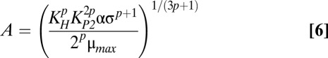
It would be useful to know the expected toxin concentration for any combination of kinetic and environmental parameter values. However, as simple as Eqs. 1–5 may appear, there is no closed-form solution for the steady-state concentrations. Nevertheless, in design space each phenotype is described by a dominant nonlinear subsystem that does have a single, well-defined steady state (37). The previous section described three cases in Fig. 1C that are visited when λ_A is increased: 3, 61, and 63. In case 3, when the dominant subsystem is solved, the concentrations of free toxin and antitoxin are described by the following equations in terms of the independent parameters:

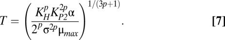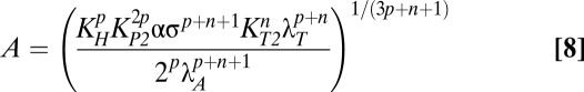
Although Eqs. 6 and 7 are nonlinear and relatively complicated, they clearly indicate that the approximate steady-state concentrations of toxin and antitoxin are not dependent on λ_A. Therefore, small deviations in λ_A from the normal operating point in case 3 should not produce significant changes in toxin or antitoxin concentrations. In fact, for any decrease in λ_A, the system remains in case 3 and therefore maintains approximately the same toxin and antitoxin levels. However, an eightfold increase in λ_A moves the system to case 63, where the steady-state concentrations are described by the following equations:

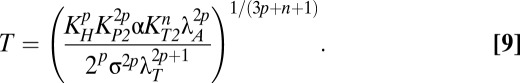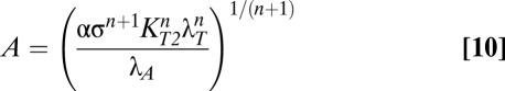
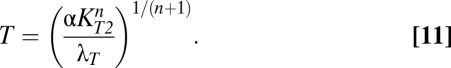
Eqs. 8 and 9 reveal that in case 63, both toxin and antitoxin concentrations are dependent on λ_A. However, if the active degradation of the antitoxin is increased enough, the system moves into case 61, where the toxin concentration is again independent of λ_A, as shown by Eqs. 10 and 11.

The steady-state concentrations for the other cases can be solved similarly. Although the solutions for A and T are nonlinear and relatively complicated, a closer inspection of Eqs. 1 and 2 reveals that the ratio of antitoxin to toxin is much simpler: A/T = σ. In fact, that ratio is the same for all cases 1–16, despite different solutions for A and T in each case. Likewise, cases 33–40 share the ratio A/T = σμ_max/λ_A. Cases 49–64 share the ratio A/T = σλ_T/λ_A, which can be found in Eqs. 8–11. The shared ratios suggest that each group of cases may exhibit similar behavior, even if the concentrations are not the same.

The steady-state concentrations for each case are plotted piecewise, as a function λ_A, in Fig. 1 D and E. For increased proteolytic activity, the free toxin concentration rises over 10-fold, after passing through a transitional region with three steady states, the hallmark of a hysteretic switch. A numerical solution to the original system of equations mirrors the sharp rise in toxin concentration and the transitional region, albeit narrower, with three steady states. In fact, any phenotypic variable can be plotted in such a piecewise fashion over the entire design space. The growth rate, defined as , is plotted in Fig. 2 A–C. The result is even more dramatic: The growth rate abruptly changes over two orders of magnitude.

Fig. 2.

Growth rate and stability. (A–C) Growth rate, based on the steady-state toxin concentration, for cases 3 and 35 (A); cases 43 and 47 (B); and cases 59, 61, and 63 (C). Black regions indicate cases that can be found in one of the other panels. Some regions have more than one steady state and therefore more than one potential growth rate. Maximum growth (blue) is expected when starting at the normal operating point (white circle) and increasing λ_A. Minimum growth (red) is expected when recovering from stress (white triangle) by decreasing λ_A. (D–F) Real part of the dominant eigenvalues for the linearized subsystem in cases 3 and 35 (D); cases 43 and 47 (E); and cases 59, 61, and 63 (F). Positive values (yellow and red) indicate instability. Slightly negative values (green) are stable, but imply relatively slow response times. Very negative values (blue) represent a stable and fast response. The operating points are consistent with Fig. 1C.

Local Stability Analysis Confirms Bistability.

A hysteretic switch has well-known stability properties: two stable steady states—low and high toxin concentrations—with an unstable intermediate steady state. In design space, the local stability of each case can be determined using well-known techniques (41). In short, a characteristic polynomial is derived from a linear approximation of the dominant subsystem. In this two-variable model, the resulting quadratic equation can be solved for the eigenvalues. Fig. 2 D–F shows the dominant eigenvalues over the entire design space. At the normal operating point in case 3, the dominant eigenvalue has a negative real part, implying the steady state is stable. An increase in λ_A forces the system through the region of multiple steady states, where the dominant eigenvalues of cases 43 and 47 always have a positive real part, implying their steady states are always unstable. For high values of λ_A, the system reaches a stable steady state in case 59, 61, or 63. In short, the system has the stability characteristics of a hysteretic switch.

The local stability can also be analyzed via the Routh stability criteria (41). Table 1 shows the Routh stability criteria for the dominant subsystem in each case. F₁ and F₂ are well-defined functions of the independent parameters and are always positive (41). The parameters n and p are the positive exponents, or kinetic orders, defined in Eqs. 1–5. In cases 3, 35, 59, 61, and 63, it is apparent that the criteria are always true, implying the system is always stable. On the other hand, the criteria in cases 43 and 47 can sometimes be false, indicating that instability is possible. It can be shown that the first criterion is false only if the second criterion is false, meaning the instability is always exponential, not oscillatory. For the estimated parameter values n = 2 and p = 2, the second criterion is false and the system, therefore, is unstable. The Routh criteria not only confirm the stability implications of the sampled eigenvalues in Fig. 2, they also mathematically describe an entire range of parameter values that can lead to a bistable hysteretic switch.

Table 1.

Two critical Routh stability criteria

Case	Criterion 1	Criterion 2
3	(2p + 1)F1 + (p + 1)F2 > 0	3p + 1 > 0
35	(2p + 1)F1 + (p + 1)F2 > 0	3p + 1 > 0
43	(2p + 1)F1 + (p + 1 − n)F2 > 0	3p + 1 − 2pn − n > 0
47	(2p + 1)F1 + (p + 1)F2 > 0	3p + 1 − 2pn > 0
59	(2p + 1)F1 + (np + 1)F2 > 0	3p + 1 > 0
61	F1 + (1 + n)F2 > 0	n + 1 > 0
63	(2p + 1)F1 + (p + 1 + n)F2 > 0	3p + 1 + n > 0

F₁ and F₂ are functions of the independent parameters and are always positive. Kinetic orders n and p are also positive. The system is stable when both criteria are true.

Design Space Boundaries Indicate Parameter Sensitivity.

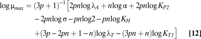
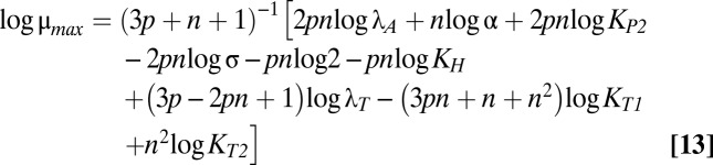
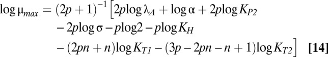
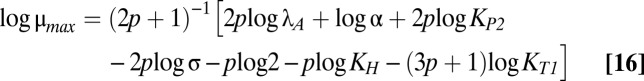
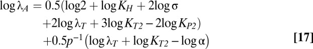
The size and shape of the bistable region in Fig. 1C are dictated by the boundaries of cases 43 and 47, which are mathematically defined by linear functions of the logarithm of the multiplicative parameters and rational functions of the exponential parameters (37). Eqs. 12–18 describe the boundary equations for lines L₁–L₇, respectively. The equations are evidently linear with respect to log μ_max and log λ_A, the axes in Fig. 1C.

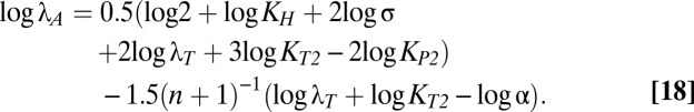L₄ is fixed with a slope of one. The slopes of L₃ and L₅ are identical and less than one. The slopes of L₁ and L₂ are greater than one. The crucial factor that appears to determine the width of the bistable region is the difference between the slope of L₅ and the slope of either L₁ or L₂. Therefore, increasing p increases the size of the bistable region, but increasing n, the strength of toxic impact, has a more dramatic effect. Indeed, Fig. S1 shows the toxin profiles when n is increased from 2 to 2.5 or 3—the bistable region grows significantly wider.

A more succinct method of describing the size of bistable region 43 is to poise the system at an operating point within the region and measure the distance to the boundaries or the tolerance of the system to large changes in the parameter values. An antitoxin half-life of 30 min poises the system in the middle of the bistable region. From there, Table 2 lists the tolerance for each parameter. The tolerances for μ_max and λ_A can be visually confirmed in Fig. 1C. The infinite tolerances indicate that any decrease in λ_T or increase in K_P1, K_T2, or n will not change regions and will therefore not change the dominant hysteretic behavior. The system is extremely tolerant to changes in α and K_P1, which is of interest because K_P1 is one of the most widely varying parameters between toxin–antitoxin systems (Table S1). It also appears that the kinetic order p, or the number of operators, can be increased to 3 or 4 without altering the dominant hysteretic behavior. On the other hand, the system is intolerant to changes in K_T1, suggesting that the kinetics of toxicity may determine whether or not the system is hysteretic. Overall, the measures of global parameter tolerance indicate that the bistable phenotype is robust and exists over a broad range of parameter values.

Table 2.

Tolerance to a fold change in each parameter

Parameter	Fold change decrease	Fold change increase
μmax	2.5	1.6
λA	1.8	3.1
λT	∞	4.7
α	10	92
σ	3.1	1.8
KH	3.2	9.6
KP1	200	∞
KP2	1.8	3.1
KT1	1.9	1.3
KT2	2.2	∞
p	4.1	2.6
n	1.1	∞

Tolerance is a measure of the change required to move the system from an initial operating point to a new region or phenotype. Here, the initial operating point is located at the center of hysteretic region 43, where (a cellular doubling time of 30 min) and (an antitoxin half-life of 30 min).

Dynamic Simulations Confirm Hysteretic Switching.

A dynamic simulation of the system, without noise, clearly exhibits hysteretic behavior. Fig. 3A shows the results of slowly increasing the rate constant of antitoxin degradation from to over twice the normal rate and then repeating the change in the opposite direction. The toxin level changes significantly at two different points on either side of a bistable region. A similar result can be seen in Fig. 3B, where μ_max is slowly decreased from to less than half the normal rate.

Fig. 3.

Dynamic simulations of toxin concentration in a single system (n = 2.5). (A and B) Deterministic simulations without noise exhibit hysteresis. (A) was slowly increased from 1 to 2.5 (blue) and then decreased from 2.5 to 1 (red). (B) was slowly decreased from 1 to 0.4 (blue) and then increased from 0.4 to 1 (red). (C and D) Stochastic simulations exhibit spontaneous switching. Five thousand members of a population were poised at either the low (white triangle) or the high (black triangle) steady-state toxin concentration for . Simulations without noise remained at the low (blue) or the high (red) steady state. Simulations with noise (d = 0.2) are shown for 500 randomly chosen members (gray), along with the population mean (green). (C) When poised at low toxin levels, members of the population infrequently transitioned to the highly toxic state. (D) When poised at the high toxin level, most of the population eventually transitioned to the normal, low-toxin state.

A recent assay for hysteresis (45) could serve as the basis for an experimental test. In brief, one of the antitoxin proteases, ClpXP for example, could be placed under the control of a gratuitous inducer. Samples taken from an unstressed culture in steady-state exponential growth could then be used to inoculate a graded series of cultures with different inducer concentrations, which represent different levels of stress. Once the inoculated cultures establish steady-state exponential growth, they could be treated with an antibiotic and assayed for the frequency of survivors (27). We predict the frequency will remain relatively constant but increase dramatically at a particular inducer concentration. For a hysteretic switch, the switching threshold depends on the history, or starting point, as shown in Fig. 3. To demonstrate the alternate threshold, a complementary experiment would have to start at the high persister frequency, conceivably by exposing the original population to a high concentration of inducer and then antibiotics, intentionally selecting for persisters. The population could then be used to inoculate a similar series of cultures. After a suitable period, the cultures could be treated with antibiotic and assayed for the frequency of survivors. In this case, we predict the dramatic shift in persister frequency will occur at a lower concentration of inducer or simulated stress.

Interestingly, the dominant eigenvalues in Fig. 2 D–F imply that the response time of the system varies by at least an order of magnitude. Fig. S2 confirms the observation, showing the difference in the system’s response to small, instantaneous changes in toxin concentration when the system is poised in the region of bistability, at either the low or the high toxin concentration. Under normal conditions, when the free toxin concentration is low, the response time is relatively rapid, as can be seen Fig. S2C. When the free toxin concentration is high, as in Fig. S2B, the response time is at least 10 times slower. Furthermore, Fig. S2D indicates that when the free toxin concentration is high, the system behaves almost linearly—the response time remains the same regardless of the magnitude of the perturbation. On the other hand, Fig. S2E shows that when toxin concentration is low, the system response varies according to the perturbation—the system is slower to return from an increase in toxin than from a decrease, an asymmetry that becomes evident in the response to small, rapid fluctuations or noise.

Spontaneous Switching Due to Stochastic Fluctuations.

Stochastic variation within the region of bistability could drive any member of a population toward either phenotype. To examine the effects of stochastic fluctuations, populations were poised at either the low or the high toxin concentration, and then each population was simulated, with and without noise. For relatively little noise, the mean behavior of the noisy population poised at the high toxin level approached the expected deterministic steady state, as can be seen in Fig. S3C. However, Fig. S3D shows that the noisy population poised at the low toxin level converged to a mean higher than the deterministic steady state, due to the asymmetric, nonlinear system response observed in Fig. S2E.

For larger stochastic fluctuations, populations exhibited spontaneous transitions from low to high toxin concentrations, as can be seen in Fig. 3C, and from high to low toxin concentrations, as can be seen in Fig. 3D. The switching can also be explained by the asymmetric system response. At the lower toxin level, the random walk of the stochastic system is biased toward higher concentrations. The larger the noise perturbation is, the slower the system responds and the greater the bias becomes. If the walk carries the system past some toxic threshold, the dynamics shift focus to the high toxin concentration, where the system is relatively sluggish and unbiased. The system becomes trapped in a slow but inevitable migration toward the highly toxic state with virtually no growth. In the highly toxic state the system wanders more slowly, albeit over a larger range, allowing for occasional reversions back to the low toxin level, as shown in Fig. 3D. The relative frequency of the switching, in either direction, can be tuned by the parameters of the system.

Dilution by Growth Can Serve as a Coordinating Signal.

Fig. 3B shows that varying the maximum growth rate constant, μ_max, even if λ_A remains the same, can switch the system between phenotypes. Such a change in μ_max could be caused by an unrelated stress or change in the environment. For example, it has been shown that bacterial signaling via indole induces persistence, likely by inducing the oxidative-stress and phage-shock pathways (46). If the maximum rate of protein production, α, is decreased in tandem with μ_max, the results are similar; however, decreasing α alone actually lowers the steady-state concentration of free toxin. It appears that when growth slows, it is the decrease in dilution, rather than the decrease in protein production, that gives rise to hysteretic behavior and the dramatic increase in toxin.

An experimental test of the growth-rate trigger could be similar to the test for hysteresis described above, save that the growth rate should be varied without changing the concentration of antitoxin protease. Samples taken from a culture in steady-state exponential growth could be used to inoculate a graded series of cultures capable of producing different steady-state exponential growth rates but similar patterns of cellular expression, including protease concentration. Although there are numerous means of changing the steady-state exponential growth rate of a culture, doing so without a large-scale change in the cellular expression pattern is a challenge. However, cells exposed to a temperature change along the linear portion of the Arrhenius plot immediately assumed the growth rate characteristic of the new temperature, suggesting a minimal change in the expression pattern (47). This is in contrast to cells undergoing a shift-up in carbon source availability, for which a significant change in the expression pattern and several generations are required before the growth rate characteristic of the new environment is achieved (48). If the challenge is overcome, we predict a dramatic shift in the frequency of persisters at a specific lower growth rate. Furthermore, if the antitoxin protease is placed under the control of a gratuitous inducer, we predict that a second series of cultures with a higher concentration of inducer—which would be represented by points on a vertical line to the right of the normal operating point in Fig. 1C—will exhibit the shift in persister frequency at a higher growth rate, demonstrating the link between λ_A and μ_max.

The results suggest how one toxin–antitoxin system could trigger another by decreasing the maximum growth rate constant μ_max. Indeed, there is experimental evidence that supports our prediction: It has been shown that Doc can induce MazF activity (49) as well as RelE activity (50), but a mechanism that accounts for the link has not been described. The indirectly triggered toxin would further decrease cell growth, potentially triggering other toxin–antitoxin systems.

Multiple Toxin–Antitoxin Systems Increase the Frequency of Persisters.

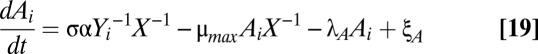
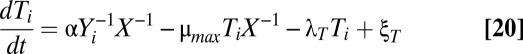
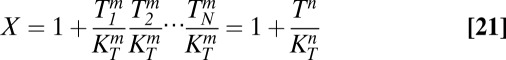
The model can be extended to account for multiple toxin–antitoxin systems, as shown in Eqs. 19–22. If each toxin affects global and cognate protein synthesis similarly, then K_T1 = K_T2 = K_T and the original equations defining X₁ and X₂, Eqs. 3 and 4, can be reduced to a single equation for X, Eq. 21. Furthermore, toxin–antitoxin systems target many different aspects of the translational machinery (51), implying that multiple toxin–antitoxin systems acting together would have a cooperative, multiplicative effect on translation, as shown in Eq. 21.

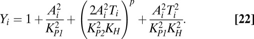Assuming the parameter values are, as shown, the same for each toxin–antitoxin system, and that the random fluctuations for each system are correlated, then the systems behave identically, or T_i = T, A_i = A, and Y_i = Y. As such, multiple systems can be analyzed using the original model with K_T1 = K_T2 and a larger Hill number, or toxic impact, n. Increasing n is equivalent to increasing the number of toxin–antitoxin systems in the model.

The marginal toxic impact, or the amount n increases for an additional toxin–antitoxin system, is influenced by several factors, including the new toxin’s independent impact, all of the toxin’s targets, and the relative toxic thresholds. Here, we simply assume that each new toxin–antitoxin system increases the aggregate toxic impact n by an average toxic impact m. Thus, if there are N toxin–antitoxin systems, and the addition of each system has an average toxic impact of 0.5, then the aggregate toxic impact will be n = 0.5N. Stochastic simulations of a population with 18 toxin–antitoxin systems, with an aggregate toxic impact of n = 9, are shown in Fig. 4A. Spontaneous switching occurred from the normal to the persistent state and back again. A histogram of μ/μ_max over the course of the simulation is bimodal, as seen in Fig. 4B, indicating that the system switched between near-maximal growth and near-zero growth, spending little time in between. On the other hand, with only 4 toxin–antitoxin systems, or n = 2, the simulations followed a unimodal distribution about a mean growth rate, and no member of the population entered the persistent state, defined as less than 20% of μ_max. Incrementally decreasing the number of toxin–antitoxin systems from 18 to 4 gradually decreased the bimodality and persister frequency. The time spent in each state was also variable, as can be seen in Fig. 4A. Two members of the population are shown that switched to the low-growth or persistent state. One reverted to normal after about 10 h and the other after about 60 h. The results suggest that persisters, like normal cells, may also hedge their bets. Some members of the persistent subpopulation could revert earlier to explore the environment—if the stress is gone, the population recovers; if the stress remains, the persistent subpopulation survives.

Fig. 4.

Stochastic simulation of multiple toxin–antitoxin systems. A total of 10⁶ members of a population were poised at the low steady-state toxin concentration, or normal growth, and simulated with stochastic noise (d = 0.2). Members that fell below 20% of μ_max (dashed line) were considered persisters. (A) For a wild-type system with 18 toxin–antitoxin systems (n = 9), simulations without noise remained at the low toxin level with high growth (blue) or the high toxin level with low growth (red). Five hundred members of the population are shown (gray) and exhibited spontaneous switching between high- and low-growth states. (B) Histogram of μ/μ_max, after reaching equilibrium, for decreasing numbers of toxin-antitoxin systems: 18 (gray), 12 (purple), 10 (light blue), 8 (red), 6 (green), and 4 (blue). (C) Population model. k_N, rate at which normal cells become persisters; k_P, rate at which persisters revert to normal cells; N, number of normal cells; P, number of persistent cells; μ_N, growth rate of normal cells; μ_P, growth rate of persistent cells. (D) Persister frequency, predicted by stochastic simulation and measured by antibiotic survival, for the wild-type cell or deletion mutants with 1–10 of the systems removed (black circles). The results are compared with recently published data (27), where type II toxin–antitoxin systems were incrementally deleted from E. coli and the resulting mutants were exposed to ciprofloxacin (blue) and ampicillin (red).

The simulations shown in Fig. 4A describe a population of constant size. In reality, the population would grow over time. Moreover, the subpopulation of persisters would grow at a fraction of the rate of normal cells. The model depicted in Fig. 4C describes such a heterogeneous, dynamic population. It has been used in the past to model subpopulations of persisters (8), as well as other cellular populations of interest (52). The number of cells in the normal subpopulation, N, grows at a rate μ_N. Likewise, the number of cells in the persistent subpopulation, P, grows at a rate μ_P. Normal cells become persisters at a rate k_N, and persisters revert at a rate k_P. The dynamics of each subpopulation can be described by the following ordinary differential equations:

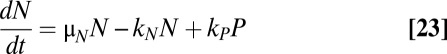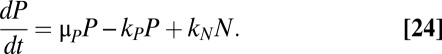It can be shown that the steady-state ratio of persisters to normal cells, R = P/N, is the solution to a quadratic equation: .

During the stochastic simulations shown in Fig. 4A, the transition rates into and out of the persistent state provided a measure for k_N and k_P. The mean growth rate of each subpopulation was used as an estimate for μ_N and μ_P. For a wild type with 18 toxin–antitoxin systems, the frequency of persisters, accounting for growth, was about 6 in 10⁵, or 0.006%. As the number of toxin–antitoxin systems was decreased, the frequency of persisters, or survivors, decreased, as shown in Fig. 4D. In particular, several toxin–antitoxin systems had to be removed before a significant decrease in the frequency of persisters occurred. From there on, removing each toxin–antitoxin system significantly and incrementally decreased the frequency of persisters. The results are in good agreement with published reports that showed the incremental deletion of type II toxin–antitoxin systems in E. coli incrementally decreased the number of persisters, regardless of the order of deletion (27). The same general response is evident even when the baseline wild-type persister frequency is tuned higher or lower via the other system parameters. An experimental test for the dependence on other system parameters would be similar to the ones we described above, with an antitoxin protease under the control of a gratuitous inducer. We predict that repeating the incremental-deletion experiment in higher concentrations of gratuitous inducer will shift the curve in Fig. 4D to the left, meaning that fewer toxin–antitoxin deletions would be required to reduce the frequency of persisters. Conversely, the result would imply that organisms in higher-stress environments might recruit more toxin–antitoxin systems to hedge their bets.

Discussion

Our results indicate that the general architecture of toxin–antitoxin systems provides the potential for a robust hysteretic switch between normal and static states. Systems that do not exhibit the necessary bistability can be coupled to produce the hysteretic behavior. The static state is characterized by virtually no growth and is reminiscent of a dormant, drug-tolerant persister, suggesting that toxin–antitoxin systems represent one of the mechanisms that contribute to persister formation. Similarly, bacteria may enter a viable but nonculturable (VBNC) state, capable of withstanding stress, tolerating antibiotics, evading detection, and reviving with full virulence (53). Although there is safety in such dormancy, it is reasonable to expect that a competitive, growing cell would postpone such a drastic change as long as possible, but once committed, act quickly and without reversion—the design principles for a hysteretic switch. Some experimental evidence suggests that deleting toxin–antitoxin cassettes does not change cell competitiveness under extremely stressful conditions (54). Indeed, our results suggest that the potential advantage may not be in a cell’s behavior at the extremes, but rather in the hysteretic, all-or-nothing switch between them.

The switch between the normal and persistent phenotypes can be driven by the proteolysis of the antitoxin, stochastic fluctuation, or a change in the growth rate. It should be noted that the threshold of the effect is dependent on the other system parameters and may therefore vary across species, strains, and environments. Furthermore, long-term adjustments to the cell physiology may compensate. Nevertheless, it is possible that the growth rate serves as a coordinating signal, ensuring that all extraordinary measures are taken in concert and cooperatively increasing the impact of multiple toxin–antitoxin systems.

Persister frequency in a wild-type population of E. coli is typically between 10⁻⁶ and 10⁻⁵ (22), although it undoubtedly varies considerably depending on the species, the strain, and the ecological niche. For example, the frequency in a biofilm of P. aeruginosa may be as high as 10⁻² (55). Our results suggest that persister frequency is a function of the overall number of toxin–antitoxin systems, their average toxic impact, the size and shape of their bistable region, and the strength of the stochastic perturbations. The size of the bistable region can be altered most dramatically by varying the overall number of toxin–antitoxin systems in a cell. The shape of the bistable region is dictated by the many parameters of the system, indicating that there are likely many ways to establish and maintain persistence, an observation that has been made elsewhere (56). Likewise, the environment can vary, and slow growth alone is not a perfect protection—metabolic stimulation, without increasing growth, can make persisters susceptible to antibiotics that target the residual translational activity (57). Simply put, the various parameters of the system can tune the frequency of persisters for a variety of contexts.

Each of our conclusions can be tested experimentally, as described in the previous sections. All of the experiments place one of the antitoxin proteases under the control of a gratuitous inducer and then use a stressed or an unstressed culture in steady state to inoculate a graded series of cultures designed to vary either the proteolytic activity or the growth rate—represented by a series of points in Fig. 1C. In every case, we predict a dramatic rise in the persister frequency at some threshold, a threshold that can then be tuned by varying another parameter in the experiment.

In summary, our model describes how toxin–antitoxin systems can give rise to a bimodal population of normal and persistent cells. The persistent subpopulation would always be present, even under normal conditions, as a bet-hedging strategy to survive a catastrophic event. The frequency of persisters in the population can be tuned for a certain niche by varying the noise strength, the relative size and position of the bistable region, the average toxic impact, and the overall number of toxin–antitoxin systems in the cell.

Methods

Model Formulation.

The references we used to create and support a general toxin–antitoxin system model are cataloged in SI Text. Fig. 1 A and B depicts the common species and their interactions. A and T represent the concentrations of monomeric antitoxin and monomeric toxin, respectively. In cases where the toxin is homodimeric, if we assume that the toxin completely folds and dimerizes at physiological concentrations, we can redefine T as the concentration of dimeric toxin, and the model remains the same. We assume the kinetics of message synthesis and degradation as well as complex formation and dissociation are relatively fast compared with the rest of the system.

In both Eqs. 1 and 2, the first and only positive term represents protein synthesis. The multiplicative factor σ represents the translational coupling between toxin and antitoxin. The overall rate of synthesis is at most α and is proportional to the fraction of unbound promoter, Y⁻¹, and the impact of the free toxin on translation, X₂⁻¹. The second term represents protein loss due to dilution, where μ_max is the maximum growth rate constant. Free toxin globally inhibits macromolecular synthesis, which slows growth and lowers the rate of dilution via X₁⁻¹. The toxin may affect global and cognate protein production differently (58), which is accounted for by the similar but separate variables X₁ and X₂. Those variables are defined in Eqs. 3 and 4, where the toxin’s impact is described by a Hill equation with a Hill number n and a concentration for half-maximal activity, either K_T1 or K_T2. The third term in Eqs. 1 and 2 represents protein loss due to active degradation, where λ_A is the rate constant of antitoxin degradation and λ_T is the rate constant of toxin degradation.

Eq. 5 describes the relative amount of bound promoter. Toxin–antitoxin systems generally have one dominant, high-affinity operator, and in this model, we ignore the weaker sites or, in the case of the cooperatively binding complex, treat the sites in aggregate. The second term represents the dimerization of the antitoxin on the surface of the promoter, with a concentration of half-maximal binding at K_P1. The third term represents the cooperative binding of the complex C to the promoter, with Hill number p and a dissociation constant K_P2 that represents increased affinity. The complex C forms when a toxin binds the antitoxin dimer at one of two independent sites with a dissociation constant K_H. The single toxin can bind to either site and hence binds with twice the affinity, or 2/K_H. The fourth term assumes that the complex D binds the operator with the same affinity as the bare dimer, or K_P1. The complex D forms when two toxins bind the antitoxin dimer with overall affinity . Together, Eqs. 1–5 form a tractable, generic model of toxin–antitoxin regulation.

Over the past decade, studies have confirmed that stochastic fluctuations in gene expression and genetic networks can have a dramatic impact (59). Noise can be tuned to advantage for specific functions or shaped and filtered by network design to minimize the negative consequences. We model stochastic noise by adding ξ_A and ξ_T to Eqs. 1 and 2, creating stochastic differential equations in Langevin form. ξ_A and ξ_T are uncorrelated white noise terms with zero mean, 〈ξ_i(t)〉 = 0, and δ-autocorrelation, 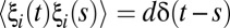, where d is proportional to the strength of the perturbation.

Parameter Estimation.

Apart from noise, the model described by Eqs. 1–5 contains 12 parameters, many of which have been experimentally measured. We used the published data for six of the best-studied toxin–antitoxin systems: kis-kid (pemIK), ccdAB, mazEF, phd-doc, relBE, and yefM-yoeB, a list that includes plasmid-borne and chromosomal toxin–antitoxin systems, some long studied and some more recently discovered. Table S1 shows the experimental values we found for each toxin–antitoxin system, as well as the final estimates we use in our model. Under optimal conditions, E. coli can double, on average, in less than 20 min (60). We assume a slightly more conservative cellular doubling time of 30 min. We also assume the Hill number p is equal to the number of repressor binding sites. Many of the parameters appear to be somewhat conserved across systems, at least within an order of magnitude.

Computational Methods.

We constructed and analyzed the system design space, using the Design Space Toolbox for MATLAB 1.0 (37). We simulated the deterministic model with the MATLAB stiff solver, ode15s. We simulated the stochastic model with our own implementation of the Euler–Maruyama method (61) in MATLAB. All tests were performed using MATLAB 7.8 (R2009a).

References

- 1.Bigger JW. Treatment of staphylococcal infections with penicillin by intermittent sterilisation. Lancet. 1944;244(6320):497–500. [Google Scholar]
- 2.Lewis K. Riddle of biofilm resistance. Antimicrob Agents Chemother. 2001;45(4):999–1007. doi: 10.1128/AAC.45.4.999-1007.2001. [DOI] [PMC free article] [PubMed] [Google Scholar]
- 3.Potera C. Forging a link between biofilms and disease. Science. 1999;283(5409):1837–1839. doi: 10.1126/science.283.5409.1837. [DOI] [PubMed] [Google Scholar]
- 4.National Institutes of Health . 1999. SBIR/STTR Study and Control of Microbial Biofilms, PA-99-084 (NIH, Bethesda, MD) [Google Scholar]
- 5.Mulcahy LR, Burns JL, Lory S, Lewis K. Emergence of Pseudomonas aeruginosa strains producing high levels of persister cells in patients with cystic fibrosis. J Bacteriol. 2010;192(23):6191–6199. doi: 10.1128/JB.01651-09. [DOI] [PMC free article] [PubMed] [Google Scholar]
- 6.Lafleur MD, Qi Q, Lewis K. Patients with long-term oral carriage harbor high-persister mutants of Candida albicans. Antimicrob Agents Chemother. 2010;54(1):39–44. doi: 10.1128/AAC.00860-09. [DOI] [PMC free article] [PubMed] [Google Scholar]
- 7.Fauvart M, De Groote VN, Michiels J. Role of persister cells in chronic infections: Clinical relevance and perspectives on anti-persister therapies. J Med Microbiol. 2011;60(Pt 6):699–709. doi: 10.1099/jmm.0.030932-0. [DOI] [PubMed] [Google Scholar]
- 8.Balaban NQ, Merrin J, Chait R, Kowalik L, Leibler S. Bacterial persistence as a phenotypic switch. Science. 2004;305(5690):1622–1625. doi: 10.1126/science.1099390. [DOI] [PubMed] [Google Scholar]
- 9.Aldridge BB, et al. Asymmetry and aging of mycobacterial cells lead to variable growth and antibiotic susceptibility. Science. 2012;335(6064):100–104. doi: 10.1126/science.1216166. [DOI] [PMC free article] [PubMed] [Google Scholar]
- 10.Lewis K. Persister cells. Annu Rev Microbiol. 2010;64(1):357–372. doi: 10.1146/annurev.micro.112408.134306. [DOI] [PubMed] [Google Scholar]
- 11.Christensen SK, Mikkelsen M, Pedersen K, Gerdes K. RelE, a global inhibitor of translation, is activated during nutritional stress. Proc Natl Acad Sci USA. 2001;98(25):14328–14333. doi: 10.1073/pnas.251327898. [DOI] [PMC free article] [PubMed] [Google Scholar]
- 12.Pedersen K, Christensen SK, Gerdes K. Rapid induction and reversal of a bacteriostatic condition by controlled expression of toxins and antitoxins. Mol Microbiol. 2002;45(2):501–510. doi: 10.1046/j.1365-2958.2002.03027.x. [DOI] [PubMed] [Google Scholar]
- 13.Christensen SK, Pedersen K, Hansen FG, Gerdes K. Toxin-antitoxin loci as stress-response-elements: ChpAK/MazF and ChpBK cleave translated RNAs and are counteracted by tmRNA. J Mol Biol. 2003;332(4):809–819. doi: 10.1016/s0022-2836(03)00922-7. [DOI] [PubMed] [Google Scholar]
- 14.Grady R, Hayes F. Axe-Txe, a broad-spectrum proteic toxin-antitoxin system specified by a multidrug-resistant, clinical isolate of Enterococcus faecium. Mol Microbiol. 2003;47(5):1419–1432. doi: 10.1046/j.1365-2958.2003.03387.x. [DOI] [PubMed] [Google Scholar]
- 15.Zhang J, Zhang Y, Zhu L, Suzuki M, Inouye M. Interference of mRNA function by sequence-specific endoribonuclease PemK. J Biol Chem. 2004;279(20):20678–20684. doi: 10.1074/jbc.M314284200. [DOI] [PubMed] [Google Scholar]
- 16.Korch SB, Hill TM. Ectopic overexpression of wild-type and mutant hipA genes in Escherichia coli: Effects on macromolecular synthesis and persister formation. J Bacteriol. 2006;188(11):3826–3836. doi: 10.1128/JB.01740-05. [DOI] [PMC free article] [PubMed] [Google Scholar]
- 17.Liu M, Zhang Y, Inouye M, Woychik NA. Bacterial addiction module toxin Doc inhibits translation elongation through its association with the 30S ribosomal subunit. Proc Natl Acad Sci USA. 2008;105(15):5885–5890. doi: 10.1073/pnas.0711949105. [DOI] [PMC free article] [PubMed] [Google Scholar]
- 18.Falla TJ, Chopra I. Joint tolerance to β-lactam and fluoroquinolone antibiotics in Escherichia coli results from overexpression of hipA. Antimicrob Agents Chemother. 1998;42(12):3282–3284. doi: 10.1128/aac.42.12.3282. [DOI] [PMC free article] [PubMed] [Google Scholar]
- 19.Keren I, Shah D, Spoering A, Kaldalu N, Lewis K. Specialized persister cells and the mechanism of multidrug tolerance in Escherichia coli. J Bacteriol. 2004;186(24):8172–8180. doi: 10.1128/JB.186.24.8172-8180.2004. [DOI] [PMC free article] [PubMed] [Google Scholar]
- 20.Vázquez-Laslop N, Lee H, Neyfakh AA. Increased persistence in Escherichia coli caused by controlled expression of toxins or other unrelated proteins. J Bacteriol. 2006;188(10):3494–3497. doi: 10.1128/JB.188.10.3494-3497.2006. [DOI] [PMC free article] [PubMed] [Google Scholar]
- 21.Shah D, et al. Persisters: A distinct physiological state of E. coli. BMC Microbiol. 2006;6(1):53. doi: 10.1186/1471-2180-6-53. [DOI] [PMC free article] [PubMed] [Google Scholar]
- 22.Moyed HS, Bertrand KP. hipA, a newly recognized gene of Escherichia coli K-12 that affects frequency of persistence after inhibition of murein synthesis. J Bacteriol. 1983;155(2):768–775. doi: 10.1128/jb.155.2.768-775.1983. [DOI] [PMC free article] [PubMed] [Google Scholar]
- 23.Yamaguchi Y, Inouye M. Regulation of growth and death in Escherichia coli by toxin-antitoxin systems. Nat Rev Microbiol. 2011;9(11):779–790. doi: 10.1038/nrmicro2651. [DOI] [PubMed] [Google Scholar]
- 24.Ramage HR, Connolly LE, Cox JS. Comprehensive functional analysis of Mycobacterium tuberculosis toxin-antitoxin systems: Implications for pathogenesis, stress responses, and evolution. PLoS Genet. 2009;5(12):e1000767. doi: 10.1371/journal.pgen.1000767. [DOI] [PMC free article] [PubMed] [Google Scholar]
- 25.Van Melderen L, Saavedra De Bast M. Bacterial toxin-antitoxin systems: More than selfish entities? PLoS Genet. 2009;5(3):e1000437. doi: 10.1371/journal.pgen.1000437. [DOI] [PMC free article] [PubMed] [Google Scholar]
- 26.Van Melderen L. Toxin-antitoxin systems: Why so many, what for? Curr Opin Microbiol. 2010;13(6):781–785. doi: 10.1016/j.mib.2010.10.006. [DOI] [PubMed] [Google Scholar]
- 27.Maisonneuve E, Shakespeare LJ, Jørgensen MG, Gerdes K. Bacterial persistence by RNA endonucleases. Proc Natl Acad Sci USA. 2011;108(32):13206–13211. doi: 10.1073/pnas.1100186108. [DOI] [PMC free article] [PubMed] [Google Scholar] [Retracted]
- 28.Dubnau D, Losick R. Bistability in bacteria. Mol Microbiol. 2006;61(3):564–572. doi: 10.1111/j.1365-2958.2006.05249.x. [DOI] [PubMed] [Google Scholar]
- 29.Voigt CA, Wolf DM, Arkin AP. The Bacillus subtilis sin operon: An evolvable network motif. Genetics. 2005;169(3):1187–1202. doi: 10.1534/genetics.104.031955. [DOI] [PMC free article] [PubMed] [Google Scholar]
- 30.Dao-Thi M-H, et al. Intricate interactions within the ccd plasmid addiction system. J Biol Chem. 2002;277(5):3733–3742. doi: 10.1074/jbc.M105505200. [DOI] [PubMed] [Google Scholar]
- 31.Lah J, et al. Energetics of structural transitions of the addiction antitoxin MazE: Is a programmed bacterial cell death dependent on the intrinsically flexible nature of the antitoxins? J Biol Chem. 2005;280(17):17397–17407. doi: 10.1074/jbc.M501128200. [DOI] [PubMed] [Google Scholar]
- 32.Rotem E, et al. Regulation of phenotypic variability by a threshold-based mechanism underlies bacterial persistence. Proc Natl Acad Sci USA. 2010;107(28):12541–12546. doi: 10.1073/pnas.1004333107. [DOI] [PMC free article] [PubMed] [Google Scholar]
- 33.Lou C, Li Z, Ouyang Q. A molecular model for persister in E. coli. J Theor Biol. 2008;255(2):205–209. doi: 10.1016/j.jtbi.2008.07.035. [DOI] [PubMed] [Google Scholar]
- 34.Savageau MA, Coelho PMBM, Fasani RA, Tolla DA, Salvador A. Phenotypes and tolerances in the design space of biochemical systems. Proc Natl Acad Sci USA. 2009;106(16):6435–6440. doi: 10.1073/pnas.0809869106. [DOI] [PMC free article] [PubMed] [Google Scholar]
- 35.Klumpp S, Zhang Z, Hwa T. Growth rate-dependent global effects on gene expression in bacteria. Cell. 2009;139(7):1366–1375. doi: 10.1016/j.cell.2009.12.001. [DOI] [PMC free article] [PubMed] [Google Scholar]
- 36.Cogan NG. Incorporating toxin hypothesis into a mathematical model of persister formation and dynamics. J Theor Biol. 2007;248(2):340–349. doi: 10.1016/j.jtbi.2007.05.021. [DOI] [PubMed] [Google Scholar]
- 37.Fasani RA, Savageau MA. Automated construction and analysis of the design space for biochemical systems. Bioinformatics. 2010;26(20):2601–2609. doi: 10.1093/bioinformatics/btq479. [DOI] [PMC free article] [PubMed] [Google Scholar]
- 38.Coelho PMBM, Salvador A, Savageau MA. Quantifying global tolerance of biochemical systems: Design implications for moiety-transfer cycles. PLoS Comput Biol. 2009;5(3):e1000319. doi: 10.1371/journal.pcbi.1000319. [DOI] [PMC free article] [PubMed] [Google Scholar]
- 39.Savageau MA, Fasani RA. Qualitatively distinct phenotypes in the design space of biochemical systems. FEBS Lett. 2009;583(24):3914–3922. doi: 10.1016/j.febslet.2009.10.073. [DOI] [PMC free article] [PubMed] [Google Scholar]
- 40.Tolla DA, Savageau MA. Phenotypic repertoire of the FNR regulatory network in Escherichia coli. Mol Microbiol. 2011;79(1):149–165. doi: 10.1111/j.1365-2958.2010.07437.x. [DOI] [PMC free article] [PubMed] [Google Scholar]
- 41.Savageau MA. 1976. Biochemical Systems Analysis: A Study of Function and Design in Molecular Biology (Addison-Wesley, Reading, MA); reprinted in Savageau MA (2009) (CreateSpace, Charleston, SC) [Google Scholar]
- 42.Kuroda A, et al. Role of inorganic polyphosphate in promoting ribosomal protein degradation by the Lon protease in E. coli. Science. 2001;293(5530):705–708. doi: 10.1126/science.1061315. [DOI] [PubMed] [Google Scholar]
- 43.Gerth U, et al. Fine-tuning in regulation of Clp protein content in Bacillus subtilis. J Bacteriol. 2004;186(1):179–191. doi: 10.1128/JB.186.1.179-191.2004. [DOI] [PMC free article] [PubMed] [Google Scholar]
- 44.Engelberg-Kulka H, et al. rexB of bacteriophage λ is an anti-cell death gene. Proc Natl Acad Sci USA. 1998;95(26):15481–15486. doi: 10.1073/pnas.95.26.15481. [DOI] [PMC free article] [PubMed] [Google Scholar]
- 45.Williams K, Savageau MA, Blumenthal RM. A bistable hysteretic switch in an activator-repressor regulated restriction-modification system. Nucleic Acids Res. 2013 doi: 10.1093/nar/gkt324. [DOI] [PMC free article] [PubMed] [Google Scholar]
- 46.Vega NM, Allison KR, Khalil AS, Collins JJ. Signaling-mediated bacterial persister formation. Nat Chem Biol. 2012;8(5):431–433. doi: 10.1038/nchembio.915. [DOI] [PMC free article] [PubMed] [Google Scholar]
- 47.Ng H, Ingraham JL, Marr AG. Damage and derepression in Escherichia coli resulting from growth at low temperatures. J Bacteriol. 1962;84(2):331–339. doi: 10.1128/jb.84.2.331-339.1962. [DOI] [PMC free article] [PubMed] [Google Scholar]
- 48.Maaløe O, Kjeldgaard NO. Control of Macromolecular Synthesis: A Study of DNA, RNA, and Protein Synthesis in Bacteria. New York: WA Benjamin; 1966. [Google Scholar]
- 49.Hazan R, Sat B, Reches M, Engelberg-Kulka H. Postsegregational killing mediated by the P1 phage “addiction module” phd-doc requires the Escherichia coli programmed cell death system mazEF. J Bacteriol. 2001;183(6):2046–2050. doi: 10.1128/JB.183.6.2046-2050.2001. [DOI] [PMC free article] [PubMed] [Google Scholar]
- 50.Garcia-Pino A, et al. Doc of prophage P1 is inhibited by its antitoxin partner Phd through fold complementation. J Biol Chem. 2008;283(45):30821–30827. doi: 10.1074/jbc.M805654200. [DOI] [PMC free article] [PubMed] [Google Scholar]
- 51.Hayes F, Van Melderen L. Toxins-antitoxins: Diversity, evolution and function. Crit Rev Biochem Mol Biol. 2011;46(5):386–408. doi: 10.3109/10409238.2011.600437. [DOI] [PubMed] [Google Scholar]
- 52.Reams AB, Kofoid E, Savageau M, Roth JR. Duplication frequency in a population of Salmonella enterica rapidly approaches steady state with or without recombination. Genetics. 2010;184(4):1077–1094. doi: 10.1534/genetics.109.111963. [DOI] [PMC free article] [PubMed] [Google Scholar]
- 53.Oliver JD. Recent findings on the viable but nonculturable state in pathogenic bacteria. FEMS Microbiol Rev. 2010;34(4):415–425. doi: 10.1111/j.1574-6976.2009.00200.x. [DOI] [PubMed] [Google Scholar]
- 54.Tsilibaris V, Maenhaut-Michel G, Mine N, Van Melderen L. What is the benefit to Escherichia coli of having multiple toxin-antitoxin systems in its genome? J Bacteriol. 2007;189(17):6101–6108. doi: 10.1128/JB.00527-07. [DOI] [PMC free article] [PubMed] [Google Scholar]
- 55.Spoering AL, Lewis K. Biofilms and planktonic cells of Pseudomonas aeruginosa have similar resistance to killing by antimicrobials. J Bacteriol. 2001;183(23):6746–6751. doi: 10.1128/JB.183.23.6746-6751.2001. [DOI] [PMC free article] [PubMed] [Google Scholar]
- 56.Allison KR, Brynildsen MP, Collins JJ. Heterogeneous bacterial persisters and engineering approaches to eliminate them. Curr Opin Microbiol. 2011;14(5):593–598. doi: 10.1016/j.mib.2011.09.002. [DOI] [PMC free article] [PubMed] [Google Scholar]
- 57.Allison KR, Brynildsen MP, Collins JJ. Metabolite-enabled eradication of bacterial persisters by aminoglycosides. Nature. 2011;473(7346):216–220. doi: 10.1038/nature10069. [DOI] [PMC free article] [PubMed] [Google Scholar]
- 58.Vesper O, et al. Selective translation of leaderless mRNAs by specialized ribosomes generated by MazF in Escherichia coli. Cell. 2011;147(1):147–157. doi: 10.1016/j.cell.2011.07.047. [DOI] [PMC free article] [PubMed] [Google Scholar]
- 59.Eldar A, Elowitz MB. Functional roles for noise in genetic circuits. Nature. 2010;467(7312):167–173. doi: 10.1038/nature09326. [DOI] [PMC free article] [PubMed] [Google Scholar]
- 60.Schaechter M, Williamson JP, Hood JR, Jr, Koch AL. Growth, cell and nuclear divisions in some bacteria. J Gen Microbiol. 1962;29(3):421–434. doi: 10.1099/00221287-29-3-421. [DOI] [PubMed] [Google Scholar]
- 61.Schwartz R. Biological Modeling and Simulation: A Survey of Practical Models, Algorithms, and Numerical Methods. Cambridge, MA: MIT Press; 2008. [Google Scholar]
Associated Data
This section collects any data citations, data availability statements, or supplementary materials included in this article.