Compressive spatial summation in human visual cortex

Abstract

Neurons within a small (a few cubic millimeters) region of visual cortex respond to stimuli within a restricted region of the visual field. Previous studies have characterized the population response of such neurons using a model that sums contrast linearly across the visual field. In this study, we tested linear spatial summation of population responses using blood oxygenation level-dependent (BOLD) functional MRI. We measured BOLD responses to a systematic set of contrast patterns and discovered systematic deviation from linearity: the data are more accurately explained by a model in which a compressive static nonlinearity is applied after linear spatial summation. We found that the nonlinearity is present in early visual areas (e.g., V1, V2) and grows more pronounced in relatively anterior extrastriate areas (e.g., LO-2, VO-2). We then analyzed the effect of compressive spatial summation in terms of changes in the position and size of a viewed object. Compressive spatial summation is consistent with tolerance to changes in position and size, an important characteristic of object representation.

functional MRI (fMRI) can be used to measure population receptive field (pRF) size in human visual cortex (Dumoulin and Wandell 2008; Smith et al. 2001). Previous models of pRFs have assumed that responses to contrast patterns sum linearly across the visual field (Dumoulin and Wandell 2008; Larsson and Heeger 2006; Thirion et al. 2006), i.e., that the response to a contrast pattern can be predicted as the sum of the responses to subregions of that pattern (Fig. 1). The validity of this assumption is important to examine, as it affects the accuracy of pRF estimates and may reveal insight into response properties at different stages of the visual map hierarchy. Assessments of linearity of spatial summation have been conducted in both electrophysiology and fMRI, but these have provided conflicting conclusions (e.g., Britten and Heuer 1999; Hansen et al. 2004; Kastner et al. 2001; Pihlaja et al. 2008). Thus the precise nature of spatial pooling, and how well the linear approximation describes physiological responses, remains unclear.

Fig. 1.

Testing spatial summation of contrast. At the left is an inflated cortical surface with sulci and gyri shaded dark and light; the locations of V1, V2, and V3 are indicated by overlays. At the right is a set of contrast patterns with a depiction of the population receptive field (pRF) of a hypothetical V1 voxel (small circle) and V3 voxel (larger circle). We test spatial summation of contrast by measuring the blood oxygenation level-dependent (BOLD) response to 2 patterns that overlap complementary portions of a pRF (partial apertures) and the BOLD response to the sum of these patterns (full aperture). If spatial summation is linear, the sum of the responses to the partial apertures should equal the response to the full aperture.

In this study, we examine spatial summation using systematic measurements of blood oxygenation level-dependent (BOLD) fMRI responses in human visual cortex to a range of spatial contrast patterns. We uncover a small nonlinear effect (subadditive spatial summation) in primary visual cortex and find that the nonlinear effect is pronounced in extrastriate maps. To account for the effect, we develop a computational model in which a compressive static nonlinearity is applied after linear spatial summation; this model substantially improves cross-validation performance compared with a linear spatial summation model.

A consequence of compressive spatial summation (CSS) is that certain stimulus transformations may change BOLD responses less than one might expect under linear spatial summation. We explore to what degree CSS accounts for the observation that responses in extrastriate cortex tend to exhibit tolerance to changes in the position and size of the retinal image cast by an object (Desimone et al. 1984; Grill-Spector et al. 1999; Gross et al. 1972; Ito et al. 1995; Perrett et al. 1982; Tovee et al. 1994). Specifically, we measure BOLD responses to objects at different positions and sizes and show that the CSS model, derived from responses to spatial contrast patterns, predicts the position and size tolerance observed in the object responses.

MATERIALS AND METHODS

Subjects

Five experienced fMRI subjects (5 males; age range 28–39 yr; mean age 32 yr) participated in this study (Supporting Table A; all supporting tables and figures are located at http://kendrickkay.net/; see endnote). All subjects had normal or corrected-to-normal visual acuity. Informed written consent was obtained from all subjects, and the experimental protocol was approved by the Stanford University Institutional Review Board. One subject (J. Winawer) was an author. Subjects participated in one to three scan sessions to measure spatial summation. Subjects also participated in one to four separate scan sessions to identify visual field maps (details in Winawer et al. 2010). Maps V3A and V3B were combined since they could not be separated in every subject.

Visual Stimuli

Display.

Stimuli were presented using an Optoma EP7155 DLP projector imaged onto a backprojection screen in the bore of the magnet. The projector operated at a resolution of 800 × 600 at 60 Hz, and the luminance response was linearized using a lookup table based on spectrophotometer measurements (maximum luminance ∼50 cd/m²). Stimuli subtended 21–30° of visual angle. A button box recorded behavioral responses. Subjects viewed the screen via a mirror mounted on the radiofrequency (RF) coil. An occluding device prevented subjects from seeing the unreflected image of the screen. A MacBook Pro computer controlled display calibration and stimulus presentation and recorded button responses using code based on Psychophysics Toolbox (Brainard 1997; Pelli 1997).

Stimuli were constructed at a resolution of 600 × 600 pixels. In all experiments, a small dot at the center of the stimulus served as a fixation point (0.2–0.5° in diameter). The color of the dot changed randomly between red, green, and blue every 5–9 s. Subjects were instructed to fixate the dot and to press a button whenever the dot changed color.

Contrast patterns (data sets 1–3).

These stimuli consisted of full-contrast (100% Michelson contrast) contrast patterns presented at different locations in the visual field (Supporting Fig. A). Contrast patterns were generated by low-pass filtering white noise at a cutoff frequency of 14 cycles per image and then thresholding the result. These patterns were designed to elicit responses from a variety of neurons with different tuning properties. All stimuli were restricted to a circular region of the display, and regions of the display not occupied by a contrast pattern were filled with neutral gray.

Three types of spatial apertures controlled the visual field location of the contrast patterns. Vertical apertures were bounded at either the right by a vertical cut or the left by a vertical cut or were unbounded. Horizontal apertures were bounded at either the top by a horizontal cut or the bottom by a horizontal cut or were unbounded. Circular apertures were centrally positioned and sized such that the edges of the apertures coincided with the cuts. Seven cuts were placed in-between the meridians and the edge of the stimulus, yielding a total of 15 cuts in each direction. To ensure dense sampling near the fovea, the spacing of the cuts increased linearly with eccentricity (for a 24° field of view, cuts would be located at 0, 0.3, 0.7, 1.3, 2.3, 3.6, 5.5, and 8.2° eccentricity). There were a total of 31 vertical + 31 horizontal + 7 circular = 69 apertures.

Aperture edges were smoothly transitioned using half-cosine functions. For edges at the vertical and horizontal cuts, the width of the transition zone was 2 pixels (0.1°) and the transition zone was centered on the cut. For edges at the bounds of the stimulus, the width of the transition zone was 11 pixels (0.4°), and the transition zone abutted the stimulus bounds.

Note that spatial responses could in principle be measured using stimuli in which multiple spatial elements are randomly presented over time (Hansen et al. 2004; Vanni et al. 2005). We chose to use simple spatial apertures for two reasons: one, aperture stimuli are simpler to interpret than random stimuli; and two, random stimuli densely stimulate the visual field on nearly every frame, which is not optimal for characterizing voxels that exhibit strong subadditive summation.

Object position and size manipulations (data sets 4–7).

These experiments measured responses to contrast patterns and objects in the same scan sessions. Models derived from the contrast responses were used to predict the object responses. For these experiments, we reduced the number of apertures used for contrast patterns from 69 to 38. This was achieved by using only 4 cuts in-between the meridians and the edge of the stimulus and by omitting circular apertures. We also modified the contrast patterns by flipping the polarity of a random 5% of the image pixels (grouped into 2- × 2-pixel chunks). The purpose of this modification was to increase power at high spatial frequencies and thus potentially elicit stronger neural responses.

To construct object stimuli, we obtained 30 presegmented objects from a previous study (Kriegeskorte et al. 2008). These objects included fruit, animals, body parts, and various small items. Objects were converted to grayscale, placed on samples of pink noise (1/f amplitude spectrum, random phase spectrum), and resized to fit various spatial apertures. One experiment (data sets 4 and 5) manipulated object position by using a 5 × 5 grid of square apertures, each 80 pixels (3.2°) on a side. Another experiment (data sets 6 and 7) manipulated object size by using 13 centrally positioned circular apertures. The radii of these apertures grew quadratically from 11 pixels (0.4°) to 300 pixels (12°) according to the expression 300x² where x is evaluated at 13 equally spaced points between 0.19 and 1. [For example, the 1st radius is 300(0.19)² = 11 pixels, the 2nd radius is 300(0.2575)² = 20 pixels, and so on.] This experiment also included a version of these apertures in which the objects were omitted, leaving only the pink-noise background.

Control experiments (data sets 6 and 7).

In one control experiment (data set 7), we tested subadditive spatial summation by presenting three vertical apertures in a slow event-related experimental design (Supporting Table A). In another control experiment (data set 7), we tested whether subadditive summation is due to a response ceiling by presenting contrast patterns at 5% Michelson contrast (2 runs; only horizontal apertures). In a 3rd control experiment (data sets 6 and 7), we again tested whether subadditive summation is due to a response ceiling, this time by comparing responses to contrast patterns against responses to a full-field aperture containing objects (1 of the stimuli used in the object experiments described above).

Alternative contrast patterns (data sets 8–10).

In a final set of control experiments, we used specially designed contrast patterns to test whether subadditive spatial summation can be explained by luminance edges between the contrast patterns and the gray background. For these experiments, stimuli were presented using a Samsung SyncMaster 305T LCD monitor (linearized luminance response; maximum luminance 117 cd/m²) and subtended 12.5–12.7° of visual angle (Supporting Table A). The small field of view is adequate for characterizing responses in V1, V2, and V3 (where pRFs are small), and results are reported for these visual field maps.

In one experiment (data set 8), summation was measured at a horizontal cut 1.5° above the horizontal meridian. Six different types of patterns were used, and summation was measured seven times for each type of pattern. Noise consisted of the original contrast patterns (cutoff frequency set to 6.25 cycles per image to compensate for the smaller display size). Band-Pass Noise consisted of patterns obtained by band-pass filtering the edges in the Noise contrast patterns (difference-of-Gaussians filter tuned to 3 cycles per degree). Checkerboard and Bars consisted of patterns constructed from square-wave gratings (spatial frequency 6.25 cycles per image); these patterns reversed contrast on each frame. Checkerboard with Spatial Gap and Bars with Spatial Gap consisted of patterns identical to Checkerboard and Bars except that a spatial gap extending between 1.0 and 2.0° above the horizontal meridian was included. The transition zone was 0.17° wide for Band-Pass Noise (corresponding to a spatial frequency of 3 cycles per degree) and 0° wide for the other types of patterns. We examined summation for voxels for which the pRFs are located within 0.5-pRF sizes from the horizontal cut and extend over the spatial gap and for which at least 50% of the pRF is contained within the bounds of the stimulus.

In a 2nd experiment (data sets 9 and 10), we repeated the main experiment (data sets 1-3) using Band-Pass Noise contrast patterns. This involved measuring responses to the full set of 69 spatial apertures (resized to the smaller field of view). To control attention, subjects performed a 1-back task on a small digit (0.25 × 0.25°) positioned at the center of the stimulus (Hallum et al. 2011). The identity of the digit (0–9) changed at 1.5 Hz, and, to minimize visual adaptation, the color of the digit alternated between black and white.

Experimental Design

We used a randomized event-related design to minimize anticipatory and attentional effects and to separate the time course of the hemodynamic response from aperture response amplitudes. Stimuli were presented in 8-s trials, one aperture per trial (Supporting Fig. A). During the 1st 3 s of a trial, the subject viewed contrast patterns (or objects) through one of the apertures (10-Hz image rate, random order). Then, for the next 5 s, the subject viewed the neutral-gray background. This 3-s ON, 5-s OFF trial structure produces robust BOLD responses, ensures sufficient gaps between apertures such that adaptation effects are minimized (Boynton and Finney 2003), and allows a large number of trials to be presented within a scan session.

For the main experiment (data sets 1-3), apertures were divided into two groups. Vertical apertures were placed in one group, horizontal apertures were placed in the other group, and the remaining apertures were distributed across these two groups. In each run, apertures from one of the groups were presented in random order (no special optimization of stimulus ordering was performed). To establish the baseline signal level, each run also included null trials in which no stimuli were presented. Two null trials were inserted at the beginning and end of each run, and 1 null trial was inserted after every 5 (or, in some cases, 6) stimulus trials. Each run lasted ∼6 min. In each scan session, vertical and horizontal runs were alternated until 5 pairs (10 runs) were collected.

MRI Data Acquisition

fMRI data for data sets 1-7 were collected at the Lucas Center at Stanford University using a GE Signa HDx 3.0T, a Nova 8-channel RF surface coil, and a Nova quadrature RF surface coil (Supporting Table A). In each scan session, 21 slices roughly parallel to the parietooccipital sulcus were defined: slice thickness 2.5 mm, slice gap 0 mm, field of view 160 × 160 mm. A T2*-weighted, single-shot, gradient-echo spiral-trajectory pulse sequence was used (Glover and Lai 1998): matrix size 64 × 64, repetition time (TR) 1.323751 s, echo time (TE) 29.7 ms, flip angle 71°, nominal spatial resolution 2.5 × 2.5 × 2.5 mm³. (The TR was matched to the refresh rate of the display such that there were exactly 6 TRs for each 8-s trial.) The TE of the 1st volume in each run was increased by 2 ms, and the phase difference between the 1st 2 volumes was used to estimate a map of the B₀ static magnetic field. To minimize respiratory-related artifacts in field maps, subjects were instructed to hold their breath for the 1st 10 s of each run. fMRI data for data sets 8-10 were collected at the Stanford Center for Cognitive and Neurobiological Imaging using a GE Signa MR750 3.0T scanner and a Nova 32-channel RF head coil. The protocol in these data sets was the same as that for data sets 1-7 except for the following characteristics: 22 slices, an echoplanar imaging (EPI) pulse sequence, TR 1.337702 s, TE 28 ms, flip angle 68°, and an alternative B₀ mapping procedure.

Data Analysis

A summary of the analysis workflow is provided in Supporting Fig. B.

Data Preprocessing

Field maps were smoothed in space and time using local linear regression (Hastie et al. 2001) and then used to guide multifrequency reconstruction of the spiral-based functional volumes (Man et al. 1997) and unwarping of the EPI-based functional volumes (Jezzard and Balaban 1995). These procedures corrected off-resonance spatial distortion artifacts and improved the run-to-run stability of the data. The first five volumes of each run were discarded to allow longitudinal magnetization to reach steady-state. Differences in slice acquisition times were corrected using sinc interpolation. Finally, automated motion correction procedures were used to correct for head motion (SPM5; rigid-body transformations). Motion parameter estimates were low-pass filtered at 1/90 Hz to remove high-frequency modulations that may have been caused by BOLD activations (Freire and Mangin 2001). No additional spatial or temporal filtering was performed. Raw scanner units were converted to units of percentage signal change by dividing by the mean signal intensity in each voxel.

The fMRI data were analyzed in two stages (Kay et al. 2008b), which we refer to as general linear model (GLM) analysis and pRF analysis. The GLM analysis deconvolves a hemodynamic response function (HRF) from the raw time-series data of each voxel to estimate the voxel response amplitude to each aperture; the pRF analysis uses these response amplitudes to estimate pRF parameters. Thus the inputs to the pRF analysis are the outputs of the GLM analysis rather than the raw time-series data. This two-stage analysis approach reduces the computational requirements of the pRF analysis and makes it easier to inspect the accuracy of pRF models. Furthermore, response amplitudes are derived from multiple trials and are therefore more reliable (less noisy) than the raw time-series data.

GLM Analysis

We fit the time-series data from each voxel using a variant of the GLM that is commonly used in fMRI analysis (a general review of the GLM can be found in Monti 2011). The model consists of several components: 1) an HRF characterizing the shape of the time course of the BOLD response to an aperture; 2) β-weights characterizing the amplitude of the BOLD response to each aperture; 3) polynomial regressors (degrees 0–3) used to estimate the baseline signal level in each run; and 4) global noise regressors designed to capture BOLD fluctuations unrelated to the stimulus.

HRF.

To ensure accurate GLM fits, we used a flexible model for the HRF at each voxel (Kay et al. 2008a). Control points were placed every 2.5 s from 0 to 20 s after trial onset and every 10 s from 20 to 50 s after trial onset. Each control point was allowed to vary freely except for the control points at 0 and 50 s, which were fixed to 0. The model of the HRF is computed by performing spline interpolation between the control points. The specific placement of the control points was chosen based on HRF measurements in pilot data and reflects a strategy in which more control points are allocated near the beginning of the trial where hemodynamic responses change at a faster rate.

Global noise regressors.

To remove the effects of spatially global BOLD fluctuations, we used a technique inspired by methods introduced by a previous study (Bianciardi et al. 2009). First, we select voxels for which the time series bear no detectable relationship to the stimulus (specifically, voxels for which the GLM has less than or equal to 0 cross-validation accuracy). Then, for each run, we extract the time series of these voxels, project out (i.e., fit and remove) the polynomial regressors from each time series, normalize each time series to have the same variance (to ensure that each time series has the same influence), and perform principal component (PC) analysis. Finally, the top PCs from each run are entered into the GLM as additional regressors. Cross-validation is used to select the number of PCs entered (typically 1–5; see Supporting Table A). We find that using global noise regressors consistently improves the cross-validation accuracy of the GLM, thus validating the method.

Model fitting.

Since the GLM used in this study is nonlinear with respect to its parameters, we used nonlinear optimization to fit the model (MATLAB Optimization Toolbox). We fit the GLM using two different resampling schemes. In GLM cross-validation, we fit the GLM five times, each time leaving out one pair of runs. In each iteration, the fitted model was used to predict stimulus-related effects (i.e., the estimated hemodynamic response to each stimulus, summed over time) in the left-out runs. Since the absolute signal level in BOLD time series cannot be accurately predicted due to signal drift (Smith et al. 1999), we projected out the polynomial regressors from both the predicted data and the measured data. We then concatenated results across the five iterations and computed the coefficient of determination (R²) between the predicted and measured data. The resulting R² value quantifies the accuracy of the GLM. In GLM bootstrapping, we fit the GLM 30 times, each time to a bootstrap sample drawn from individual runs. (Bootstrapping individual data points would be improper since noise in BOLD time series is correlated over time; see Friman and Westin 2005.) Each bootstrap sample was balanced by including exactly 5 vertical and 5 horizontal runs. To ensure proper handling of noise correlations across voxels, the same bootstrap samples were used for different voxels. Bootstrap results were used to estimate standard errors on model parameters.

pRF Analysis

CSS model.

A pRF model is an encoding model (Kay 2011; Naselaris et al. 2011) that characterizes the relationship between a contrast image (indicating the location of the stimulus) and the response from a local population of neurons. We used a pRF model that generates a predicted response by computing a weighted [isotropic 2-dimensional (2-D) Gaussian] sum of the contrast image and then applying a static power-law nonlinearity. This can be expressed formally as:

$$\text{RESP}=\text{g}\times {\left[{\displaystyle \int \text{S}\left(x,y\right)\text{G}\left(x,y\right)dxdy}\right]}^n$$

$$\text{G}\left(x,y\right)=e^{-\frac{{\left(x-x\prime \right)}^2+{\left(y-y\prime \right)}^2}{2{\sigma }^2}}$$

where RESP is the predicted response, g is a gain parameter, x and y represent different positions in the visual field, S is the contrast image, G is the Gaussian, n is an exponent parameter, x′ and y′ are parameters controlling the position of the Gaussian, and σ is a parameter controlling the standard deviation of the Gaussian. We use a power-law nonlinearity because it captures a wide range of behaviors using a single parameter that is easy to interpret. Empirically, we find that the power-law exponent is consistently <1; thus we refer to the model as the CSS model.

The CSS model involves two nonlinearities: 1) an implicit initial nonlinearity that converts luminance to contrast; and 2) the compressive static nonlinearity that is applied after spatial summation. Note that linearity of spatial summation does not depend on the weighting function (isotropic 2-D Gaussian) assumed in the model. All linear pRF models that predict the response as a weighted sum of the contrast image necessarily imply linear spatial summation; this is the case even if the weights are anisotropic (Kumano and Uka 2010; Motter 2009; Palmer et al. 2012; Schall et al. 1986) or if the weights include a negative surround (Cavanaugh et al. 2002; Kraft et al. 2005; Nurminen et al. 2009; Zuiderbaan et al. 2012). However, it may be possible to enhance the performance of the CSS model by incorporating a different weighting function into the model. Also note that for the purposes of this study, the compressive static nonlinearity is only intended to characterize response properties pertaining to spatial summation. We speculate, however, that the nonlinearity may be a general mechanism that governs the temporal domain as well: the nonlinearity might serve as an explanation of adaptation effects where the response to two successive stimuli is less than the sum of the responses to the stimuli presented individually (Krekelberg et al. 2006).

Model fitting.

We fit the CSS model to each voxel using the β-weights (BOLD response amplitudes) estimated in the GLM. Model fitting was performed using nonlinear optimization (MATLAB Optimization Toolbox). The stimulus was prepared by downsampling the apertures to 100 × 100 pixels. Stimulus values ranged from 0 (no contrast) to 1 (full contrast). To ensure reasonable model estimates, we constrained the x′ and y′ parameters to be within a region three times the size of the stimulus and the σ and n parameters to be positive. The x′ and y′ parameters were seeded with 50.5 (the center of the stimulus), the σ parameter was seeded with 100, and the g parameter was seeded with 1. To avoid local minima, we first optimized the x′, y′, σ, and g parameters with the n parameter fixed at 0.5 and then optimized all parameters simultaneously. A post hoc linear approximation was used to convert pixel units into degrees of retinal angle.

The CSS model was fit using 3 different resampling schemes. In pRF bootstrapping, we fit the CSS model 30 times, once for each set of β-weights obtained in bootstrapping the GLM model. Bootstrap results were used to estimate standard errors on model parameters. In pRF full-fit, we fit the CSS model to a single set of β-weights obtained by taking the mean across GLM bootstraps. This set of β-weights reflects the full data set and therefore provides the best estimates of model parameters. The pRF of a voxel refers to the CSS model estimated using the full-fit resampling scheme unless otherwise indicated. In pRF cross-validation, we fit the CSS model to the single set of β-weights using leave-one-out cross-validation. Cross-validation controls for overfitting and provides unbiased estimates of model accuracy.

Model accuracy.

The accuracy of the CSS model was quantified as the coefficient of determination (R²) between the cross-validated predictions of the β-weights and the measured β-weights:

$$R^2=100\times \left[1-\frac{{\displaystyle \sum }{\left(\text{MODEL}-\text{DATA}\right)}^2}{{\displaystyle \sum {\text{DATA}}^2}}\right]$$

where MODEL indicates the predicted weights and DATA indicates the measured weights. This R² value indicates the percentage of variance (relative to 0% signal change) that is explained by the CSS model. R² provides a more accurate assessment of accuracy than r² (the square of Pearson's correlation coefficient) because r² is not sensitive to mismatches in offset and gain. Also, note that quantifying variance with respect to 0 (instead of the mean) makes it easier to compare the R² metric across different sets of data (which may differ in their means).

Linear model.

To assess the importance of the static nonlinearity in the CSS model, we fit a version of the model in which the exponent parameter is fixed to 1. This modification eliminates the static nonlinearity and reduces the model to a linear model. The linear model and the CSS model were fit independently to the data. The linear model is identical to the model used previously by Dumoulin and Wandell (2008).

Definition of pRF Size

In the CSS model, there is an interaction between the size of the Gaussian and the static nonlinearity. For example, a model associated with a small Gaussian can nevertheless respond strongly to stimuli far from the Gaussian if the static nonlinearity is highly compressive. We propose to define pRF size in terms of the predicted response to a point stimulus (spot) placed at different positions in the visual field.

The predicted response of the CSS model to point stimuli has a Gaussian profile:

$$\text{M}\left(x,y\right)=\text{g}\times \text{G}{\left(x,y\right)}^n\propto e^{-\frac{{{\left(x-x\prime \right)}^{}}^2+{\left(y-y\prime \right)}^2}{2{\sigma }^2}n}$$

$${=e}^{-\frac{{{\left(x-x\prime \right)}^{}}^2+{\left(y-y\prime \right)}^2}{2{\left(\frac{\sigma }{\sqrt{n}}\right)}^2}}$$

where M is a map of responses and other variables are as defined earlier. We define pRF size, σ_size, to be the standard deviation of the Gaussian profile:

$${\sigma }_{\text{size}}=\frac{\sigma }{\sqrt{n}}.$$

Our definition of pRF size is based on input-output characteristics and could be applied to any pRF model. For a model for which the predicted response to point stimuli does not have a Gaussian profile, we could simply stipulate that pRF size is the standard deviation of a Gaussian function fitted to the actual profile.

Noise Ceiling

The noise ceiling is defined as the maximum accuracy that a model can be expected to achieve given the level of noise in the data (David and Gallant 2005; Sahani and Linden 2003). The noise ceiling depends solely on the signal-to-noise ratio of the data and is independent of the specific model being evaluated. In our case, the data of interest are the β-weights estimated in the GLM and the model of interest is a pRF model that has been fitted to these β-weights.

We performed Monte Carlo simulations to calculate the noise ceiling. In these simulations, we generate a known signal and noisy measurements of this signal and then calculate the R² between the signal and the measurements. This computational approach directly quantifies the noise ceiling assuming that both the signal and the noise level are known. For our data, the signal is not directly known (since the data include both signal and noise). To carry out the simulations, we make the simplifying assumptions that the signal and the noise are each distributed according to a normal distribution and that the noise is zero mean.

The first step in the simulations was to collect the β-weights and their standard errors. Standard errors on individual β-weights are relatively noisy given that each stimulus was presented just five times. We thus calculated the pooled standard error and took this to be the standard deviation of the normal distribution characterizing the noise:

$$\text{NOISESD}=\sqrt{\text{mean}\left({\beta }_{\sigma }^2\right)}$$

where NOISESD is the noise standard deviation and β_σ represents the standard errors on the β-weights. Next, we calculated the mean of the β-weights and took this to be the mean of the normal distribution characterizing the signal:

$$\text{SIGNALMN}=\text{mean}\left({\beta }_{\mu }\right)$$

where SIGNALMN is the signal mean and β_μ represents the β-weights. To estimate the standard deviation of the signal distribution, we subtracted the amount of variance attributable to noise from the total amount of variance in the data, forced the result to be nonnegative, and then computed the square root:

$$\text{SIGNALSD}=\sqrt{\max \left[0,\mathrm{var}\left({\beta }_{\mu }\right)-{\text{NOISESD}}^2\right]}$$

where SIGNALSD is the signal standard deviation. Finally, we generated a signal by drawing random values from the signal distribution, generated a noisy measurement of this signal by summing the signal and random values drawn from the noise distribution, and calculated the R² between the signal and the measurement. We performed 500 simulations (50 signals, 10 measurements per signal) and took the median R² value to be the noise ceiling.

The noise ceiling is inherently a stochastic quantity: the accuracy of a perfect model will vary from data set to data set simply due to randomness in the measurement noise. For example, a perfect model could achieve a cross-validation R² of 100% if the noise just happens to be 0 for each data point. The stochasticity of the noise ceiling is reflected in the variability of the R² values obtained in the Monte Carlo simulations. The noise ceiling is taken to be the median R² value across simulations and should be interpreted as the accuracy that a perfect model is expected to achieve on average given the level of noise in the data.

Voxel Selection

Results were restricted to voxels that satisfy the following requirements. First, voxels must have a complete set of data, i.e., must not have moved outside of the imaged volume during the scan session. Second, voxels must be located in one of the identified visual field maps. Third, voxels must have positive GLM cross-validation accuracy. Finally, voxels must have GLM β-weights that are positive on average. This requirement excludes peripheral voxels that typically exhibit negative BOLD responses to centrally presented stimuli (Shmuel et al. 2006; Smith et al. 2004). Voxels in each visual field map were pooled across subjects. Unless otherwise indicated, error bars represent ±1 SE (68% confidence intervals) across voxels and were obtained using bootstrapping.

Public Data Sets and Software Code

Example data sets and code implementing the CSS model are provided at http://kendrickkay.net/socmodel/.

RESULTS

To investigate spatial summation, we measured BOLD responses in human visual cortex while subjects viewed a series of spatial contrast patterns. Contrast patterns were high-contrast, black-and-white noise patterns seen through a systematic set of vertical, horizontal, and circular apertures. Sixty-nine distinct apertures were presented in random order a total of five times each. The data were preprocessed to estimate the BOLD response amplitude of each voxel to each aperture.

Subadditive Spatial Summation

The experimental design included apertures that form complementary pairs (e.g., left aperture, right aperture), and we used these pairs to assess whether responses sum linearly over space. For each aperture pair, we selected voxels for which the pRFs are located near the boundary between the two apertures and computed a summation ratio by dividing the response to a full aperture covering the entire visual field by the sum of the responses to the two apertures. If spatial summation is linear, the summation ratio should equal 1. The summation ratio is <1 in all identified visual field maps, indicating that the response to the full aperture is smaller than predicted by linear spatial summation (Fig. 2). The summation ratio is closest to 1 in V1 and is substantially less than 1 in extrastriate maps. We confirmed the reproducibility of these results with a control experiment in which subadditive summation can be directly observed in the measured BOLD time series (Fig. 3A).

Fig. 2.

Spatial summation is subadditive throughout visual cortex. A: example tests of spatial summation. The black bars indicate the responses of an example V1 voxel and V3 voxel to the apertures shown below. In both cases, the response to the full aperture is less than the linear prediction (horizontal line). The summation ratio, defined as the response to the full aperture divided by the linear prediction, is 0.78 for the V1 voxel and 0.59 for the V3 voxel. B: median summation ratio in different visual field maps. We calculated the median summation ratio across aperture pairs located within 0.5-pRF sizes from the pRF center. (If an aperture pair is distant from a pRF, 1 aperture would have no influence on the response, and linear summation would hold trivially; see Supporting Fig. C for details; all supporting tables and figures are located at http://kendrickkay.net/; also see endnote.) Responses are subadditive in all visual field maps and especially so in extrastriate maps.

Fig. 3.

Control experiments for subadditive spatial summation. A: slow event-related design using a full-field aperture and apertures covering either the left or right hemifield. Data are BOLD time series averaged across V1 voxels with pRF centers within 10 angular degrees from the vertical meridian. The response to the full aperture is smaller than the sum of the responses to the left and right apertures (dotted line), indicating subadditive summation. B: low-contrast experiment. A ceiling on the BOLD response might exist due to saturation of neural activity or limitations on hemodynamic mechanisms (Buxton et al. 2004). To test whether a response ceiling explains subadditive summation, we presented contrast patterns at low contrast. In all visual field maps, subadditive summation occurs at low contrast, and the response to the full aperture at low contrast is smaller than the corresponding response at high contrast (Supporting Table B). Hence, subadditivity at low contrast cannot be explained by a response ceiling. C: object experiment. To test whether subadditivity at high contrast is due to a response ceiling, we compared the response to the full aperture containing contrast patterns with the response to the same aperture containing objects. In all maps except V1 and V2, the object stimulus elicits a higher response than the contrast stimulus (Supporting Table B). This provides further evidence that subadditivity is not due to a response ceiling.

A potential explanation of subadditive summation is that the response to the full aperture is lower than the linear prediction simply because the response is already at the maximum level. However, control experiments show that subadditivity is not due to a response ceiling: subadditivity occurs even at low contrast (Fig. 3B), and it is possible to evoke responses that are even higher than the response to the full aperture (Fig. 3C).

Another potential explanation of subadditive summation is that the partial apertures contain luminance edges between the contrast patterns and the gray background, whereas such edges are not present in the full aperture. Since edges drive neural responses, this might explain why the response to the full aperture is lower than expected. To test this possibility, we measured summation for alternative contrast patterns that minimize the edge effect and confirmed that subadditive summation still occurs (Fig. 4). We also performed a full set of measurements using alternative contrast patterns and reproduce the main results of the present paper (Supporting Fig. G).

Fig. 4.

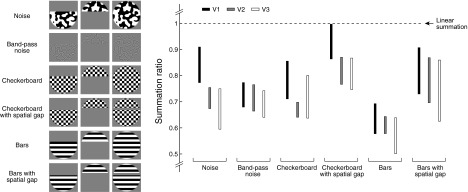
Summation for other types of contrast patterns. A trivial explanation for subadditivity is that the partial apertures contain luminance edges at the boundary between the contrast pattern and the gray background, whereas the full aperture does not. To test this explanation, we measured summation using the original pattern (Noise), a band-pass pattern that lacks the previously described luminance edges (Band-Pass Noise), patterns for which the previously described luminance edges are present in both the partial and full apertures (Checkerboard, Bars), and patterns that include a spatial gap such that the same luminance edges are present in the partial and full apertures (Checkerboard with Spatial Gap, Bars with Spatial Gap). The median summation ratios in V1, V2, and V3 are shown [error bars indicate standard error across general linear model (GLM) bootstraps]. In all cases, subadditive summation occurs, arguing against the edge explanation. There appears to be some variation in summation ratio across stimulus types; accounting for these dependencies on stimulus type is a direction for future research. (For additional experiments ruling out the edge explanation, see Supporting Fig. G.)

Edges between the contrast patterns and the gray background cannot explain subadditive summation, but it is possible that these edges may contribute to the size of the subadditive effect. For example, inserting a spatial gap such that the same luminance edges are present in the partial and full apertures reduces the level of subadditivity (Fig. 4). However, this manipulation changes the visual field regions that are summated, which might also explain the different summation results. In general, the use of a spatial gap avoids edge effects but complicates the design of stimuli that systematically sample different regions of the visual field. The goal of this paper is not to test summation for one particular case (e.g., a single location in the visual field, a single gap size, etc.) but rather to use systematic measurements of spatial responses to develop a general model of the relationship between the location of the stimulus and the observed responses. We address this issue next.

CSS Model

A pRF is the region of the visual field within which stimuli evoke responses from a local population of neurons (Dumoulin and Wandell 2008; Victor et al. 1994). Existing models of pRFs use linear weights applied to the stimulus contrast (Dumoulin and Wandell 2008; Larsson and Heeger 2006; Thirion et al. 2006) and therefore predict linear, not subadditive, summation. Note that linearity is implied even if weights are arranged in a center-surround configuration with negative weights in the surround.

To account for subadditive summation, we propose a new pRF model. In this model, the stimulus is represented as a contrast image (indicating the location of the stimulus), and the response is computed as a weighted (isotropic 2-D Gaussian) sum of the contrast image followed by a static power-law nonlinearity (Fig. 5). The key component of the model is the nonlinearity: if the exponent of the power-law nonlinearity is <1, the nonlinearity is compressive, and small amounts of overlap between the stimulus and the pRF produce large responses. This behavior predicts subadditive summation. We refer to the model as the CSS model.

Fig. 5.

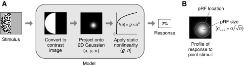
Compressive spatial summation (CSS) model. A: schematic of CSS model. The model starts with a contrast image that represents the location of the stimulus in the visual field. To predict the response, the contrast image is weighted and summed using an isotropic 2-dimensional (2-D) Gaussian and then transformed by a static power-law nonlinearity. When the power-law exponent is <1, the nonlinearity is compressive, and the model predicts subadditive spatial summation. B: definition of pRF size and location. The response of the CSS model to point stimuli placed at different visual field positions has a Gaussian profile. We define pRF size to be the standard deviation of this Gaussian profile, σ_size. We represent pRF location using a circle with radius 2σ_size.

We evaluated the CSS model by comparing it with a version of the model in which the power-law exponent is fixed to 1. This simplified model implies strict linear spatial summation. We independently fit the CSS model and the linear model to the responses of each voxel using cross-validation and quantified model accuracy as the percentage of variance explained (R²). Although the models are nested, there is no guarantee that the CSS model will have higher cross-validation accuracy than the linear model: this will occur only if the effect captured by the exponent is sufficiently large and there are sufficient data to estimate the exponent accurately. If the effect of the exponent is small or if data quality is poor, the exponent parameter in the CSS model may degrade cross-validation accuracy due to overfitting.

The CSS model outperforms the linear model in all visual field maps (Fig. 6). In V1, the improvement is modest, indicating that the linear model is a reasonable characterization of the responses for the range of stimuli tested. In extrastriate maps, the improvement is substantial, consistent with the strong subadditive effects found in these maps. Furthermore, the absolute performance of the CSS model is quite high: on average, the model predicts 84% of the response variance (median R² across voxels). This is only slightly lower than the maximum performance that can be expected given the level of noise in the data (noise ceiling), which is 89% of the response variance (median R² across voxels). Detailed examination of the data and model fits confirms the accuracy of the CSS model (Supporting Figs. D and E).

Fig. 6.

CSS model outperforms linear model. A: cross-validation accuracy in different visual field maps. Vertical bars indicate the median accuracy across voxels in each map. Horizontal lines indicate the median noise ceiling. The CSS model outperforms the linear model in all maps (P < 1e−8, 2-tailed sign test). Increases in accuracy are more substantial in extrastriate maps than in V1. B: cross-validation accuracy for individual voxels. Each dot compares the accuracies of the 2 models for a single voxel.

In V1, the performance improvement provided by the CSS model is modest, at an increase of 1.3% variance. This may seem inconsistent with the fact that the summation ratio in V1 is substantially less than 1, at 0.78. The reason for this apparent discrepancy is that the summation ratio is computed from the subset of data that specifically tests linearity (aperture pairs defined by cuts that are located near pRF centers), whereas model accuracy is a summary metric that reflects the entire data set. Since V1 pRFs are small, only a few apertures cut through the pRF for any given V1 voxel, and so the overall performance of the linear model is only slightly lower than that of the CSS model.

Examination of Model Parameters

The CSS model parameters provide a compact summary of the response properties of individual voxels. One parameter of interest is pRF size. Consistent with previous studies (Amano et al. 2009; Dumoulin and Wandell 2008; Kay et al. 2008b; Larsson and Heeger 2006; Smith et al. 2001; Winawer et al. 2010), pRF size increases with eccentricity and increases in extrastriate visual field maps (Fig. 7A). However, there are quantitative differences between the size estimates here and those of previous studies. One difference is that linear functions relating eccentricity and size pass close to the origin in our study but not in previous studies. This is likely due to the fact that the stimuli used in this study sampled the foveal visual field more finely than the stimuli used in previous studies. The fact that size scales nearly perfectly with eccentricity is interesting and suggests a fundamental similarity between response properties at the fovea and those at the periphery. Another difference is that our size estimates are generally smaller. This is explained by the fact that previous studies used linear pRF models, which can overestimate pRF size when the underlying system exhibits nonlinear, subadditive behavior (for examples, see Supporting Figs. D and E).

Fig. 7.

Model parameters vary systematically across visual cortex. A: changes in pRF size. We fit a line relating eccentricity and size for each visual field map. The band around each line indicates a bootstrap estimate of the standard error (see Supporting Fig. F for details). Size increases with eccentricity and increases in extrastriate maps. B: changes in pRF exponent. The median exponent in each map is plotted against the average size at 5° (deg) of eccentricity. In all maps, the median exponent is <1, indicating a compressive nonlinearity. Maps with larger sizes tend to have smaller exponents.

A new parameter introduced by the CSS model is pRF exponent, which governs the amount of subadditive summation exhibited by a given voxel. Consistent with the spatial summation tests, the median exponent is <1 in all visual field maps and is smaller in extrastriate maps than in V1 (Fig. 7B). Given that maps with larger pRF sizes tend to have smaller exponents, we wondered whether the change in exponent across maps could be explained by changes in pRF size. Exploiting the fact that there exists a range of pRF sizes within individual visual field maps, we compared exponents across maps while holding size constant. We find that after controlling for size, V3 pRFs are still more compressive than V2 pRFs, which in turn are still more compressive than V1 pRFs (Supporting Fig. F). This indicates that the change in compression from map to map is distinct from the change in size.

Implications for Object Stimuli

We developed the CSS model based on responses to simple spatial contrast patterns. Here, we ask how well the model can generalize in predicting responses to more natural stimuli. We were particularly interested in the implications of CSS for the observation that extrastriate responses exhibit tolerance to changes in object position and size (Desimone et al. 1984; Perrett et al. 1982). To explore this connection, we measured BOLD responses to object stimuli at various positions and sizes and assessed how well the CSS model accounts for these data.

Objects were placed on textured backgrounds and viewed through apertures of different positions and sizes. To generate predictions from the CSS model, we simply took the apertures, which reflect the spatial extent of the objects, and passed these apertures through the CSS model. Because the CSS model is a purely spatial model, it does not account for the fact that in certain extrastriate maps, objects are particularly effective at driving responses compared with noise patterns (Malach et al. 1995). We therefore included a nonnegative scale factor on the overall gain of the predicted responses while leaving the remaining model parameters untouched (location, size, and exponent). This procedure quantifies the accuracy of the CSS model in predicting the relative but not the absolute response amplitudes.

In all visual field maps, the relative responses to objects of different sizes are well-predicted by the CSS model (Fig. 8). In particular, the CSS model successfully captures the fact that responses in anterior maps (e.g., LO-2, VO-2) are relatively unaffected by the changes in object size that we evaluated. The performance of the CSS model does not quite reach the noise ceiling in V1 and V2; this may be due to negative BOLD responses that are not accounted for by the model (Fig. 8C). In additional experiments, we found that the CSS model also performs well at accounting for relative responses to objects varying in position (Supporting Fig. H).

Fig. 8.

CSS model is consistent with tolerance to changes in object size. We tested how well the CSS model, estimated from responses to spatial contrast patterns, predicts responses to objects that vary in size. Note that the model predicts only the relative pattern of responses, not the overall gain in responses (see main text). A: sample stimulus frames. Objects were presented on textured backgrounds within circular apertures of different sizes. B: model accuracy in different visual field maps (format same as Fig. 6A). The accuracy of the CSS model is close to the noise ceiling. C: data and model predictions. For visualization purposes, we normalize the responses from each voxel to unit length and plot the median response to each object size as a black bar (error bars indicate the interquartile range). In anterior maps, responses are relatively unaffected by changes in object size, and the CSS model successfully reproduces this effect.

DISCUSSION

Potential Sources of Subadditive Spatial Summation

We have shown that the BOLD response to a contrast pattern is less than the sum of the BOLD responses to individual parts of the contrast pattern. This subadditive spatial summation may reflect nonlinearities in neural response properties or might reflect nonlinearities in the coupling between neural activity and the hemodynamic response (Cardoso et al. 2012; Heeger and Ress 2002; Logothetis and Wandell 2004; Magri et al. 2011). In particular, because nearby points in the visual field are mapped to nearby points on cortex, whether the hemodynamic response reflects a linear spatial convolution of neural activity is especially pertinent (Boynton 2011).

We attribute subadditivity primarily to the neural response for three reasons. First, the amount of subadditivity varies between visual field maps (Figs. 2B and 7B). If the effect were entirely explained by hemodynamic coupling, one would not expect a systematic relationship with visual field map. Second, similar subadditive effects have been observed in neuronal responses in MT (Britten and Heuer 1999; Heuer and Britten 2002). Third, we recently performed electrocorticography (ECoG) in V1–V4 of human visual cortex and have found that subadditive spatial summation also occurs in these measurements (Winawer et al. 2013). ECoG measures population activity at the millimeter scale (similar to BOLD fMRI) but is not influenced by the coupling between neural activity and the hemodynamic response.

However, we recognize that from BOLD measurements alone, it is difficult to make inferences regarding the precise level of CSS in neural signals. First, there is a diverse array of cell types in cortex. Each may be governed by its own spatial summation rules and may couple differently to the BOLD signal. Second, there are different aspects of neural activity (e.g., synaptic potentials, action potentials), and each may exhibit different spatial summation properties. Third, there may be scatter in the receptive field positions of neurons within a voxel, which tends to produce summation results at the population level that are more linear than that at the level of individual neurons (discussed further below). These various issues should be taken into account when interpreting the CSS effects found in this paper.

Previous Studies of Spatial Summation

Hansen et al. (2004) reported linear spatial summation of V1 BOLD responses, whereas we find subadditive summation in V1 (median summation ratio 0.78). This discrepancy may be due to the difference in voxel sizes used in the two studies. Hansen et al. (2004) used 3.5- × 3.5- × 4.1-mm³ voxels, whereas the present study used isotropic 2.5-mm voxels, smaller in volume by a factor of three. Large voxels are likely to include neurons responsive to only one of the apertures being summed, especially in V1 where receptive fields are small. Thus large voxel size may tend to produce spatial summation results that are more linear. Another reason for the discrepancy may be that the summation tests in the present study were performed using aperture pairs located near pRF centers, thereby providing more sensitive tests of summation (Supporting Fig. C). Finally, the use of simultaneously presented spatial components may have distorted the estimates of responses to individual components, given the linear regression analysis used in that study (further discussed below).

Subadditive spatial summation is consistent with the previous observation that the estimated V1 BOLD response to a central patch is reduced when using a multifocal design that involves surrounding patches (Pihlaja et al. 2008). Because responses to simultaneous patches are smaller than the responses predicted by linear summation, the estimate of the response to the central patch is biased downward in the linear regression analysis of multifocal data. Subadditive summation is also consistent with the finding that in V1 and more so in extrastriate maps, the response to simultaneously presented stimuli is smaller than the response to the stimuli when sequentially presented (Kastner et al. 2001). Simultaneous presentation engages subadditive spatial summation, whereas sequential presentation does not. Finally, our summation results are consistent with recent BOLD measurements of nonlinear spatial effects throughout visual cortex (Vanni and Rosenstrom 2011). This study also found increasingly nonlinear effects in anterior visual areas and proposed an alternative, information-theoretic explanation for the findings. Our study extends these previous results (see also results from EEG: Vanni et al. 2004) by performing systematic measurements of spatial summation for many visual field maps and by developing a computational model that predicts responses at the level of single voxels.

We examined spatial summation of simple contrast patterns in this study. However, summation characteristics may vary depending on the specific type of stimuli that are summed. An example is summation of two parts of a solid luminance disc: since cortical responses are primarily driven by contrast (Engel et al. 1997), the response to the full disc is likely to be quite small compared with the responses to the partial discs. Another example is summation of multiple objects, which has been the focus of a number of studies (e.g., Kastner et al. 2001; Macevoy and Epstein 2009; Reddy et al. 2009; Reynolds et al. 1999; Zoccolan et al. 2005). These studies typically find that in certain extrastriate regions, the response to two objects presented simultaneously is the average of the responses to the objects presented individually. In particular, the response to an effective object presented alone is usually reduced when a less-effective object is presented nearby. The CSS model does not account for this effect, since stimulating more of the visual field always produces a higher response from the CSS model. Expanding the explanatory power of the CSS model is a direction for future research.

Distinction Between Subadditive Spatial Summation and Contrast Saturation

Contrast saturation refers to the well-established fact that responses in visual cortex plateau beyond a certain contrast level (Albrecht and Hamilton 1982; Boynton et al. 1999; Sclar et al. 1990; Tootell et al. 1998). There is a parallel between contrast saturation and subadditive spatial summation: just as a small amount of contrast is sufficient to evoke a large response, a small amount of spatial stimulation is also sufficient to evoke a large response. However, the two phenomena are conceptually distinct: in theory, it is possible for responses to exhibit contrast saturation but linear spatial summation or to exhibit linear contrast response but subadditive spatial summation. Consider a receptive field composed of subunits that saturate with contrast but are summed linearly across space. This receptive field will exhibit contrast saturation but approximately linear spatial summation. Thus the fact that responses in visual cortex exhibit subadditive spatial summation is an empirical finding that is distinct from contrast saturation. Interestingly, we find an increase in subadditivity in anterior visual field maps, which mirrors the increase in contrast saturation in anterior maps (Avidan et al. 2002; Kastner et al. 2004; Tootell et al. 1998). This suggests that the two effects may be tightly linked and that it may useful to explore and develop a general model that simultaneously accounts for both contrast saturation and subadditive spatial summation (e.g., a model that computes the standard deviation of pixel luminance values over a local portion of the visual field and then applies a compressive nonlinearity, a model based on divisive normalization, etc.).

Relationship to Divisive Normalization

Divisive normalization is a nonlinear computation that is widely used to model neuronal responses (Carandini and Heeger 2011; Heeger 1992). Here, we link divisive normalization to CSS by showing that under certain assumptions, divisive normalization at the neuronal level implies CSS at the population level. First, consider the following formulation of divisive normalization:

$${\text{output}}_i=\frac{{\text{neuron}}_i}{\sigma +{\displaystyle \sum _k}{\text{neuron}}_k}$$

where output_i is the final output from the ith neuron, neuron_i is the unnormalized response of the ith neuron, σ is a semisaturation constant, and k ranges over a local population of neurons (the normalization pool). Let us assume that the neurons in the normalization pool mutually inhibit each other. Then, the pooled activity of the population of neurons in the normalization pool is:

$$\text{pooled}\text{\hspace{0.17em}activity}={\displaystyle \sum _k}{\text{output}}_k=\frac{{\displaystyle \sum _k}{\text{neuron}}_k}{\sigma +{\displaystyle \sum _k}{\text{neuron}}_{\text{k}}}=f\left({\displaystyle \sum _k}{\text{neuron}}_k\right)\text{ where }f\left(x\right)=\frac{x}{\sigma +x}\mathrm{.}$$

This shows that at the population level, the effect of normalization is to apply a compressive nonlinearity (represented by f) to the sum of the unnormalized responses of the neurons in the normalization pool (represented by x).

To connect these theoretical considerations to spatial summation, we can identify the x term in the previous equation as representing space, that is, the amount of spatial overlap between a stimulus and a pRF. As the overlap between the stimulus and the pRF increases, the pooled activity of the normalization pool is expected to increase according to a compressive function. This response behavior is the core of the CSS model. Thus we can view CSS as a specific instantiation of the general computation of divisive normalization.

The divisive nonlinearity described above can be approximated, through suitable choice of parameters, by the power-law nonlinearity used in the CSS model. However, the approximation is not exact, and we wondered whether some gain in performance might be achieved by changing the form of the static nonlinearity in the CSS model. Division and exponentiation are in fact special cases of the general model of neural computation described by Kouh and Poggio (2008). We therefore tested several nonlinearities with different levels of generality. The median cross-validated R² for the original power-law nonlinearity f(x) = xⁿ is 84.3% ± 0.2 SE. In contrast, the pure divisive nonlinearity $f\left(x\right)=\frac{x}{\sigma +x}$ achieves 83.2% ± 0.2 SE, the mixed divisive nonlinearity $f\left(x\right)=\frac{x^n}{{\sigma }^n+x^n}$ achieves 84.1% ± 0.2 SE, and the general nonlinearity $f\left(x\right)=\frac{x^n}{{\sigma }^n+x^m}$ achieves 83.5% ± 0.2 SE. The fact that alternative nonlinearities do not improve performance indicates that the power-law nonlinearity is sufficient for the data we have. Further elaborations of the CSS model to account for additional phenomena (e.g., surround suppression) may require the nonlinearity to be divisive in form.

Models of Position and Size Tolerance in the Visual System

Compared with posterior visual field maps, anterior maps have larger pRF sizes and smaller (more compressive) pRF exponents (Fig. 7B). The combination of these two properties implies that responses in anterior maps should show reduced sensitivity to changes in the position and size of a viewed object, and we have confirmed that this is the case (Fig. 8C and Supporting Fig. H). The increase in tolerance that we observe mirrors the results of a recent study that compared neural responses in macaque V4 and IT to a common set of object stimuli and demonstrated that IT responses exhibit greater tolerance to changes in position, size, and context (Rust and Dicarlo 2010).

A number of object-recognition models that address position and size tolerance have been proposed (for example, Epshtein et al. 2008; Fukushima 1980; Perrett and Oram 1993; Pinto et al. 2009; Rolls and Milward 2000). We discuss here HMAX, an influential model in both computer and biological vision (Riesenhuber and Poggio 1999; Serre et al. 2007). The CSS model is largely compatible with the basic features of the HMAX model (feedforward model with increasing nonlinearity and spatial pooling at successive stages), but there are several differences. One difference is that the HMAX model is explicitly hierarchical such that responses are transformed through a sequence of computations. In contrast, the CSS model is designed to predict responses of each voxel directly from the stimulus. This stimulus-referred approach simplifies parameter estimation and interpretation of the model. It is possible, however, to reformulate the CSS model using a hierarchical architecture similar to that of the HMAX model (Fig. 9). This reformulation shows how the spatial nonlinearity of the CSS model can be split into several sequential stages, each stage implementing the same local computation.

Fig. 9.

CSS model can be expressed in hierarchical form. We simulated a hierarchical model in which the stimulus (layer 0, resolution 16 × 16) initiates responses in 3 layers of units (layers 1-3, resolution 16 × 16). The response of a unit at any given layer is computed by projecting responses of the previous layer onto an isotropic 2-D Gaussian and then transforming the result by a compressive power-law function. This can be expressed formally by R_k(i,j) = [∫R_k−1(x,y)G(x,y)dxdy]ⁿ where R_k(i,j) indicates the response of the unit positioned at (i,j) in layer k, x and y represent different positions in the visual field, and G indicates a 2-D isotropic Gaussian centered at (i,j) (the standard deviation of the Gaussian was set to 0.75, and n was set to 0.5). We computed the response of this model to a set of contrast patterns and fit the stimulus-referred CSS model to each unit in the hierarchical model. The pRF estimates for 3 example units (black dots) are shown on the right. These pRFs explain >99.99% of the response variance, demonstrating that the stimulus-referred model and the hierarchical model make the same predictions. Notice that size and compression increase at higher levels of the hierarchy, mirroring the experimental results (Fig. 7B). Because the local computations are the same at each layer, the increase in size and compression is due to the hierarchical model architecture.

Another difference between the HMAX and CSS models is the specific way in which tolerance is achieved. The HMAX model achieves tolerance by applying the MAX operation to the responses of model units that encode a specific image feature at slightly different positions and scales. The CSS model achieves tolerance by applying a compressive nonlinearity after summation of contrast across space. The difference in nonlinearity is not critically important, as CSS can be approximated using the MAX operation. However, because the CSS model addresses only space and not specific image features, the model has few free parameters, and this has enabled us to test the model against experimental measurements directly. Our data sets are freely available (see materials and methods), and we welcome efforts to consider how well alternative models of visual processing account for these experimental measurements.

Extending the CSS Model to Account for Stimulus Selectivity

Selectivity is an important concept that is complementary to tolerance. Theories of object representation (DiCarlo et al. 2012; Riesenhuber and Poggio 1999; Ullman 1996) propose that visual responses should exhibit not only tolerance to variation in object format (such as object position, size, and viewpoint), but also selectivity for certain objects over others. Examining our data, we find preliminary evidence that voxel responses indeed conform to the selectivity-tolerance framework, exhibiting tolerance for spatial variation while also exhibiting selectivity for certain stimulus types (Supporting Fig. I). This is consistent with the finding that neurons in macaque inferotemporal cortex maintain object preferences over changes in position and size (Ito et al. 1995; Tovee et al. 1994).

The CSS model is a simple spatial model, and we have shown that the response properties of the model are consistent with the position and size tolerance observed in several extrastriate visual field maps. However, an important limitation of the CSS model is that it does not explain selectivity, that is, why certain stimulus types drive responses more strongly than others. A complete model of object representation must address both selectivity and tolerance, and in future research it will be fruitful to measure responses to stimuli that vary along not only the dimension of space (e.g., location and size), but also other dimensions (e.g., the specific image features at a given location and size). We will then be in a position to extend the CSS model to account for stimulus selectivity. One promising strategy is to integrate the CSS model with filters that operate on arbitrary images (Kay et al. 2008b); this is a line of research that we have pursued in a follow-up study (Kay et al. 2013).

GRANTS

This work was supported by National Eye Institute Grants K99-EY-022116 (J. Winawer) and R01-EY-03164 (B. A. Wandell).

DISCLOSURES

No conflicts of interest, financial or otherwise, are declared by the author(s).

ENDNOTE

At the request of the authors, readers are herein alerted to the fact that additional materials related to this manuscript may be found at the institutional web site of the authors, which at the time of publication they indicate is: http://kendrickkay.net/. These materials are not a part of this manuscript and have not undergone peer review by the American Physiological Society (APS). APS and the journal editors take no responsibility for these materials, for the web site address, or for any links to or from it.

AUTHOR CONTRIBUTIONS

K.N.K. conducted the experiment and analyzed the data; J.W. assisted with data collection and retinotopic mapping; J.W. and A.M. provided conceptual guidance; K.N.K. and B.A.W. wrote the paper; K.N.K., J.W., A.M., and B.A.W. discussed the results and commented on the manuscript.

REFERENCES

- Albrecht DG, Hamilton DB. Striate cortex of monkey and cat: contrast response function. J Neurophysiol 48: 217–237, 1982 [DOI] [PubMed] [Google Scholar]
- Amano K, Wandell BA, Dumoulin SO. Visual field maps, population receptive field sizes, and visual field coverage in the human MT+ complex. J Neurophysiol 102: 2704–2718, 2009 [DOI] [PMC free article] [PubMed] [Google Scholar]
- Avidan G, Harel M, Hendler T, Ben-Bashat D, Zohary E, Malach R. Contrast sensitivity in human visual areas and its relationship to object recognition. J Neurophysiol 87: 3102–3116, 2002 [DOI] [PubMed] [Google Scholar]
- Bianciardi M, van Gelderen P, Duyn JH, Fukunaga M, de Zwart JA. Making the most of fMRI at 7 T by suppressing spontaneous signal fluctuations. Neuroimage 44: 448–454, 2009 [DOI] [PMC free article] [PubMed] [Google Scholar]
- Boynton GM. Spikes, BOLD, attention, and awareness: a comparison of electrophysiological and fMRI signals in V1. J Vis 11: 12, 2011 [DOI] [PMC free article] [PubMed] [Google Scholar]
- Boynton GM, Demb JB, Glover GH, Heeger DJ. Neuronal basis of contrast discrimination. Vision Res 39: 257–269, 1999 [DOI] [PubMed] [Google Scholar]
- Boynton GM, Finney EM. Orientation-specific adaptation in human visual cortex. J Neurosci 23: 8781–8787, 2003 [DOI] [PMC free article] [PubMed] [Google Scholar]
- Brainard DH. The Psychophysics Toolbox. Spat Vis 10: 433–436, 1997 [PubMed] [Google Scholar]
- Britten KH, Heuer HW. Spatial summation in the receptive fields of MT neurons. J Neurosci 19: 5074–5084, 1999 [DOI] [PMC free article] [PubMed] [Google Scholar]
- Buxton RB, Uludag K, Dubowitz DJ, Liu TT. Modeling the hemodynamic response to brain activation. Neuroimage 23, Suppl 1: S220–S233, 2004 [DOI] [PubMed] [Google Scholar]
- Carandini M, Heeger DJ. Normalization as a canonical neural computation. Nat Rev Neurosci 13: 51–62, 2011 [DOI] [PMC free article] [PubMed] [Google Scholar]
- Cardoso MM, Sirotin YB, Lima B, Glushenkova E, Das A. The neuroimaging signal is a linear sum of neurally distinct stimulus- and task-related components. Nat Neurosci 15: 1298–1306, 2012 [DOI] [PMC free article] [PubMed] [Google Scholar]
- Cavanaugh JR, Bair W, Movshon JA. Nature and interaction of signals from the receptive field center and surround in macaque V1 neurons. J Neurophysiol 88: 2530–2546, 2002 [DOI] [PubMed] [Google Scholar]
- David SV, Gallant JL. Predicting neuronal responses during natural vision. Network 16: 239–260, 2005 [DOI] [PubMed] [Google Scholar]
- Desimone R, Albright TD, Gross CG, Bruce C. Stimulus-selective properties of inferior temporal neurons in the macaque. J Neurosci 4: 2051–2062, 1984 [DOI] [PMC free article] [PubMed] [Google Scholar]
- DiCarlo JJ, Zoccolan D, Rust NC. How does the brain solve visual object recognition? Neuron 73: 415–434, 2012 [DOI] [PMC free article] [PubMed] [Google Scholar]
- Dumoulin SO, Wandell BA. Population receptive field estimates in human visual cortex. Neuroimage 39: 647–660, 2008 [DOI] [PMC free article] [PubMed] [Google Scholar]
- Engel SA, Glover GH, Wandell BA. Retinotopic organization in human visual cortex and the spatial precision of functional MRI. Cereb Cortex 7: 181–192, 1997 [DOI] [PubMed] [Google Scholar]
- Epshtein B, Lifshitz I, Ullman S. Image interpretation by a single bottom-up top-down cycle. Proc Natl Acad Sci USA 105: 14298–14303, 2008 [DOI] [PMC free article] [PubMed] [Google Scholar]
- Freire L, Mangin JF. Motion correction algorithms may create spurious brain activations in the absence of subject motion. Neuroimage 14: 709–722, 2001 [DOI] [PubMed] [Google Scholar]
- Friman O, Westin CF. Resampling fMRI time series. Neuroimage 25: 859–867, 2005 [DOI] [PubMed] [Google Scholar]
- Fukushima K. Neocognitron: a self organizing neural network model for a mechanism of pattern recognition unaffected by shift in position. Biol Cybern 36: 193–202, 1980 [DOI] [PubMed] [Google Scholar]
- Glover GH, Lai S. Self-navigated spiral fMRI: interleaved versus single-shot. Magn Reson Med 39: 361–368, 1998 [DOI] [PubMed] [Google Scholar]
- Grill-Spector K, Kushnir T, Edelman S, Avidan G, Itzchak Y, Malach R. Differential processing of objects under various viewing conditions in the human lateral occipital complex. Neuron 24: 187–203, 1999 [DOI] [PubMed] [Google Scholar]
- Gross CG, Rocha-Miranda CE, Bender DB. Visual properties of neurons in inferotemporal cortex of the macaque. J Neurophysiol 35: 96–111, 1972 [DOI] [PubMed] [Google Scholar]
- Hallum LE, Landy MS, Heeger DJ. Human primary visual cortex (V1) is selective for second-order spatial frequency. J Neurophysiol 105: 2121–2131, 2011 [DOI] [PMC free article] [PubMed] [Google Scholar]
- Hansen KA, David SV, Gallant JL. Parametric reverse correlation reveals spatial linearity of retinotopic human V1 BOLD response. Neuroimage 23: 233–241, 2004 [DOI] [PubMed] [Google Scholar]
- Hastie T, Tibshirani R, Friedman JH. The Elements of Statistical Learning: Data Mining, Inference, and Prediction. New York: Springer, 2001 [Google Scholar]
- Heeger DJ. Normalization of cell responses in cat striate cortex. Vis Neurosci 9: 181–197, 1992 [DOI] [PubMed] [Google Scholar]
- Heeger DJ, Ress D. What does fMRI tell us about neuronal activity? Nat Rev Neurosci 3: 142–151, 2002 [DOI] [PubMed] [Google Scholar]
- Heuer HW, Britten KH. Contrast dependence of response normalization in area MT of the rhesus macaque. J Neurophysiol 88: 3398–3408, 2002 [DOI] [PubMed] [Google Scholar]
- Ito M, Tamura H, Fujita I, Tanaka K. Size and position invariance of neuronal responses in monkey inferotemporal cortex. J Neurophysiol 73: 218–226, 1995 [DOI] [PubMed] [Google Scholar]
- Jezzard P, Balaban RS. Correction for geometric distortion in echo planar images from B0 field variations. Magn Reson Med 34: 65–73, 1995 [DOI] [PubMed] [Google Scholar]
- Kastner S, De Weerd P, Pinsk MA, Elizondo MI, Desimone R, Ungerleider LG. Modulation of sensory suppression: implications for receptive field sizes in the human visual cortex. J Neurophysiol 86: 1398–1411, 2001 [DOI] [PubMed] [Google Scholar]
- Kastner S, O'Connor DH, Fukui MM, Fehd HM, Herwig U, Pinsk MA. Functional imaging of the human lateral geniculate nucleus and pulvinar. J Neurophysiol 91: 438–448, 2004 [DOI] [PubMed] [Google Scholar]
- Kay KN, Winawer J, Rokem A, Mezer A, Wandell BA. A two-stage cascade model of BOLD responses in human visual cortex. PLoS Comput Biol. First published 2013; 10.1371/journal.pcbi.1003079 [DOI] [PMC free article] [PubMed] [Google Scholar]
- Kay KN. Understanding visual representation by developing receptive-field models. In: Visual Population Codes: Towards a Common Multivariate Framework for Cell Recording and Functional Imaging, edited by Kriegeskorte N, Kreiman G. Cambridge, MA: MIT Press, 2011 [Google Scholar]
- Kay KN, David SV, Prenger RJ, Hansen KA, Gallant JL. Modeling low-frequency fluctuation and hemodynamic response timecourse in event-related fMRI. Hum Brain Mapp 29: 142–156, 2008a [DOI] [PMC free article] [PubMed] [Google Scholar]
- Kay KN, Naselaris T, Prenger RJ, Gallant JL. Identifying natural images from human brain activity. Nature 452: 352–355, 2008b [DOI] [PMC free article] [PubMed] [Google Scholar]
- Kouh M, Poggio T. A canonical neural circuit for cortical nonlinear operations. Neural Comput 20: 1427–1451, 2008 [DOI] [PubMed] [Google Scholar]
- Kraft A, Schira MM, Hagendorf H, Schmidt S, Olma M, Brandt SA. fMRI localizer technique: efficient acquisition and functional properties of single retinotopic positions in the human visual cortex. Neuroimage 28: 453–463, 2005 [DOI] [PubMed] [Google Scholar]
- Krekelberg B, Boynton GM, van Wezel RJ. Adaptation: from single cells to BOLD signals. Trends Neurosci 29: 250–256, 2006 [DOI] [PubMed] [Google Scholar]
- Kriegeskorte N, Mur M, Ruff DA, Kiani R, Bodurka J, Esteky H, Tanaka K, Bandettini PA. Matching categorical object representations in inferior temporal cortex of man and monkey. Neuron 60: 1126–1141, 2008 [DOI] [PMC free article] [PubMed] [Google Scholar]
- Kumano H, Uka T. The spatial profile of macaque MT neurons is consistent with Gaussian sampling of logarithmically coordinated visual representation. J Neurophysiol 104: 61–75, 2010 [DOI] [PubMed] [Google Scholar]
- Larsson J, Heeger DJ. Two retinotopic visual areas in human lateral occipital cortex. J Neurosci 26: 13128–13142, 2006 [DOI] [PMC free article] [PubMed] [Google Scholar]
- Logothetis NK, Wandell BA. Interpreting the BOLD signal. Annu Rev Physiol 66: 735–769, 2004 [DOI] [PubMed] [Google Scholar]
- Macevoy SP, Epstein RA. Decoding the representation of multiple simultaneous objects in human occipitotemporal cortex. Curr Biol 19: 943–947, 2009 [DOI] [PMC free article] [PubMed] [Google Scholar]
- Magri C, Logothetis NK, Panzeri S. Investigating static nonlinearities in neurovascular coupling. Magn Reson Imaging 29: 1358–1364, 2011 [DOI] [PubMed] [Google Scholar]
- Malach R, Reppas JB, Benson RR, Kwong KK, Jiang H, Kennedy WA, Ledden PJ, Brady TJ, Rosen BR, Tootell RB. Object-related activity revealed by functional magnetic resonance imaging in human occipital cortex. Proc Natl Acad Sci USA 92: 8135–8139, 1995 [DOI] [PMC free article] [PubMed] [Google Scholar]
- Man LC, Pauly JM, Macovski A. Multifrequency interpolation for fast off-resonance correction. Magn Reson Med 37: 785–792, 1997 [DOI] [PubMed] [Google Scholar]
- Monti MM. Statistical analysis of fMRI time-series: a critical review of the GLM approach. Front Hum Neurosci 5: 28, 2011 [DOI] [PMC free article] [PubMed] [Google Scholar]
- Motter BC. Central V4 receptive fields are scaled by the V1 cortical magnification and correspond to a constant-sized sampling of the V1 surface. J Neurosci 29: 5749–5757, 2009 [DOI] [PMC free article] [PubMed] [Google Scholar]
- Naselaris T, Kay KN, Nishimoto S, Gallant JL. Encoding and decoding in fMRI. Neuroimage 56: 400–410, 2011 [DOI] [PMC free article] [PubMed] [Google Scholar]
- Nurminen L, Kilpelainen M, Laurinen P, Vanni S. Area summation in human visual system: psychophysics, fMRI, and modeling. J Neurophysiol 102: 2900–2909, 2009 [DOI] [PubMed] [Google Scholar]
- Palmer CR, Chen Y, Seidemann E. Uniform spatial spread of population activity in primate parafoveal V1. J Neurophysiol 107: 1857–1867, 2012 [DOI] [PMC free article] [PubMed] [Google Scholar]
- Pelli DG. The VideoToolbox software for visual psychophysics: transforming numbers into movies. Spat Vis 10: 437–442, 1997 [PubMed] [Google Scholar]
- Perrett DI, Oram MW. Neurophysiology of shape processing. Image Vis Comput 11: 317–333, 1993 [Google Scholar]
- Perrett DI, Rolls ET, Caan W. Visual neurones responsive to faces in the monkey temporal cortex. Exp Brain Res 47: 329–342, 1982 [DOI] [PubMed] [Google Scholar]
- Pihlaja M, Henriksson L, James AC, Vanni S. Quantitative multifocal fMRI shows active suppression in human V1. Hum Brain Mapp 29: 1001–1014, 2008 [DOI] [PMC free article] [PubMed] [Google Scholar]
- Pinto N, Doukhan D, DiCarlo JJ, Cox DD. A high-throughput screening approach to discovering good forms of biologically inspired visual representation. PLoS Comput Biol 5: e1000579, 2009 [DOI] [PMC free article] [PubMed] [Google Scholar]
- Reddy L, Kanwisher NG, VanRullen R. Attention and biased competition in multi-voxel object representations. Proc Natl Acad Sci USA 106: 21447–21452, 2009 [DOI] [PMC free article] [PubMed] [Google Scholar]
- Reynolds JH, Chelazzi L, Desimone R. Competitive mechanisms subserve attention in macaque areas V2 and V4. J Neurosci 19: 1736–1753, 1999 [DOI] [PMC free article] [PubMed] [Google Scholar]
- Riesenhuber M, Poggio T. Hierarchical models of object recognition in cortex. Nat Neurosci 2: 1019–1025, 1999 [DOI] [PubMed] [Google Scholar]
- Rolls ET, Milward T. A model of invariant object recognition in the visual system: learning rules, activation functions, lateral inhibition, and information-based performance measures. Neural Comput 12: 2547–2572, 2000 [DOI] [PubMed] [Google Scholar]
- Rust NC, Dicarlo JJ. Selectivity and tolerance (“invariance”) both increase as visual information propagates from cortical area V4 to IT. J Neurosci 30: 12978–12995, 2010 [DOI] [PMC free article] [PubMed] [Google Scholar]
- Sahani M, Linden JF. How linear are auditory cortical responses? In: Advances in Neural Information Processing Systems 15, edited by Becker S, Thrun S, Obermayer K. Cambridge, MA: MIT Press, 2003, p. 109–116 [Google Scholar]
- Schall JD, Perry VH, Leventhal AG. Retinal ganglion cell dendritic fields in old-world monkeys are oriented radially. Brain Res 368: 18–23, 1986 [DOI] [PubMed] [Google Scholar]
- Sclar G, Maunsell JH, Lennie P. Coding of image contrast in central visual pathways of the macaque monkey. Vision Res 30: 1–10, 1990 [DOI] [PubMed] [Google Scholar]
- Serre T, Wolf L, Bileschi S, Riesenhuber M, Poggio T. Robust object recognition with cortex-like mechanisms. IEEE Trans Pattern Anal Mach Intell 29: 411–426, 2007 [DOI] [PubMed] [Google Scholar]
- Shmuel A, Augath M, Oeltermann A, Logothetis NK. Negative functional MRI response correlates with decreases in neuronal activity in monkey visual area V1. Nat Neurosci 9: 569–577, 2006 [DOI] [PubMed] [Google Scholar]
- Smith AM, Lewis BK, Ruttimann UE, Ye FQ, Sinnwell TM, Yang Y, Duyn JH, Frank JA. Investigation of low frequency drift in fMRI signal. Neuroimage 9: 526–533, 1999 [DOI] [PubMed] [Google Scholar]
- Smith AT, Singh KD, Williams AL, Greenlee MW. Estimating receptive field size from fMRI data in human striate and extrastriate visual cortex. Cereb Cortex 11: 1182–1190, 2001 [DOI] [PubMed] [Google Scholar]
- Smith AT, Williams AL, Singh KD. Negative BOLD in the visual cortex: evidence against blood stealing. Hum Brain Mapp 21: 213–220, 2004 [DOI] [PMC free article] [PubMed] [Google Scholar]
- Thirion B, Duchesnay E, Hubbard E, Dubois J, Poline JB, Lebihan D, Dehaene S. Inverse retinotopy: inferring the visual content of images from brain activation patterns. Neuroimage 33: 1104–1116, 2006 [DOI] [PubMed] [Google Scholar]
- Tootell RB, Hadjikhani NK, Vanduffel W, Liu AK, Mendola JD, Sereno MI, Dale AM. Functional analysis of primary visual cortex (V1) in humans. Proc Natl Acad Sci USA 95: 811–817, 1998 [DOI] [PMC free article] [PubMed] [Google Scholar]
- Tovee MJ, Rolls ET, Azzopardi P. Translation invariance in the responses to faces of single neurons in the temporal visual cortical areas of the alert macaque. J Neurophysiol 72: 1049–1060, 1994 [DOI] [PubMed] [Google Scholar]
- Ullman S. High-Level Vision: Object Recognition and Visual Cognition. Cambridge, MA: MIT Press, 1996 [Google Scholar]
- Vanni S, Dojat M, Warnking J, Delon-Martin C, Segebarth C, Bullier J. Timing of interactions across the visual field in the human cortex. Neuroimage 21: 818–828, 2004 [DOI] [PubMed] [Google Scholar]
- Vanni S, Henriksson L, James AC. Multifocal fMRI mapping of visual cortical areas. Neuroimage 27: 95–105, 2005 [DOI] [PubMed] [Google Scholar]
- Vanni S, Rosenstrom T. Local non-linear interactions in the visual cortex may reflect global decorrelation. J Comput Neurosci 30: 109–124, 2011 [DOI] [PubMed] [Google Scholar]
- Victor JD, Purpura K, Katz E, Mao B. Population encoding of spatial frequency, orientation, and color in macaque V1. J Neurophysiol 72: 2151–2166, 1994 [DOI] [PubMed] [Google Scholar]
- Winawer J, Horiguchi H, Sayres RA, Amano K, Wandell BA. Mapping hV4 and ventral occipital cortex: the venous eclipse. J Vis 10: 1–22, 2010 [DOI] [PMC free article] [PubMed] [Google Scholar]
- Winawer J, Kay KN, Foster B, Rauschecker A, Parvizi J, Wandell BA. Asynchronous broadband signals are the principal source of the BOLD response in human visual cortex. Curr Biol. First published 2013; 10.1016/j.cub.2013.05.001 [DOI] [PMC free article] [PubMed] [Google Scholar]
- Zoccolan D, Cox DD, DiCarlo JJ. Multiple object response normalization in monkey inferotemporal cortex. J Neurosci 25: 8150–8164, 2005 [DOI] [PMC free article] [PubMed] [Google Scholar]
- Zuiderbaan W, Harvey BM, Dumoulin SO. Modeling center-surround configurations in population receptive fields using fMRI. J Vis 12: 10, 2012 [DOI] [PubMed] [Google Scholar]