Abstract
This review provides a comprehensive description of the self-guided Langevin dynamics (SGLD) and the self-guided molecular dynamics (SGMD) methods and their applications. Example systems are included to provide guidance on optimal application of these methods in simulation studies. SGMD/SGLD has enhanced ability to overcome energy barriers and accelerate rare events to affordable time scales. It has been demonstrated that with moderate parameters, SGLD can routinely cross energy barriers of 20 kT at a rate that molecular dynamics (MD) or Langevin dynamics (LD) crosses 10 kT barriers. The core of these methods is the use of local averages of forces and momenta in a direct manner that can preserve the canonical ensemble. The use of such local averages results in methods where low frequency motion “borrows” energy from high frequency degrees of freedom when a barrier is approached and then returns that excess energy after a barrier is crossed. This self-guiding effect also results in an accelerated diffusion to enhance conformational sampling efficiency. The resulting ensemble with SGLD deviates in a small way from the canonical ensemble, and that deviation can be corrected with either an on-the-fly or a post processing reweighting procedure that provides an excellent canonical ensemble for systems with a limited number of accelerated degrees of freedom. Since reweighting procedures are generally not size extensive, a newer method, SGLDfp, uses local averages of both momenta and forces to preserve the ensemble without reweighting. The SGLDfp approach is size extensive and can be used to accelerate low frequency motion in large systems, or in systems with explicit solvent where solvent diffusion is also to be enhanced. Since these methods are direct and straightforward, they can be used in conjunction with many other sampling methods or free energy methods by simply replacing the integration of degrees of freedom that are normally sampled by MD or LD.
The conformational search problem
Conformational search is a problem for simulation systems where populated states are either separated by less populated conformations, which can be energy barriers or kinetic bottlenecks, or are spread across a long distance that corresponds to significant conformational changes. In biological systems, conformational search is very challenging because biological molecules such as proteins or DNA are macromolecules with huge conformational space and numerous energy barriers. Biological relevant events, such as protein folding (Dobson & Karplus 1999), ligand binding, conformational signal transduction, etc., occur in a time scale far exceeding that accessible by current realistic simulations (Adcock & McCammon 2006).
The conformation search problem for macromolecules has been the subject of intense efforts for many decades. There are numerous methods and approaches, each with various strengths and weaknesses, and there are several review articles that survey these methods rather well (Christen & Van Gunsteren 2008; Foloppe & Chen 2009; Gao et al 2008; Klenin et al 2011; Liwo et al 2008; Norberg & Nilsson 2003; Tai 2004).
Among the many methods for efficient conformational search, the self-guided molecular dynamic (SGMD) (Wu & Wang 1998; 1999) and the self-guided Langevin dynamics (SGLD) (Wu & Brooks 2003; Wu & Brooks 2011a; 2011b) simulation methods are somewhat unique. The term “self-guided” refers to the manner in which the information learned during a simulation is used to enhance the conformational search of the very same simulation. The core of these methods is the use of local averages of force and momenta in a as a guiding force that accelerates barrier crossing in a manner that can also can preserve the canonical ensemble. Even though these methods have been discussed in reviews by Norberg and Nilsson (Norberg & Nilsson 2003), Tai (Tai 2004), and Christen and van Gunsteren (Christen & Van Gunsteren 2008), this review presents a more complete description of the method including recent developments.
To better understand how SGLD relates to the many other sampling and search methods, it is worthwhile to categorize sampling methods by considering the following eight questions:
Are structures found by iterative sampling, or are structures found with a construction/library/build-up/genetic procedure?
Is the method efficient relative to standard MD? How much so?
Is the canonical ensemble directly generated? or via reweighting? or is a non-ensemble collection of structures generated?
Is the trajectory continuous?
Is the time scale preserved? or is the time scale lost via acceleration?
Is the sampling method direct? or indirect via exchanges or couplings?
Does there need to be a predetermination of enhanced degrees of freedom? or are all degrees of freedom enhanced?
Is there an effective maximum barrier height? or is all space explored?
For each of these eight questions, we contrast SGLD with alternative methods.
1. Are structures found by iterative sampling, or are structures found with a construction/library/build-up/genetic procedure?
The standard techniques of Metropolis Monte Carlo (MC), molecular dynamics (MD), and Langevin dynamics (LD) are typical iterative sampling methods that are designed to sample the canonical ensemble by default. By contrast, there is a wide variety of build-up (Budin et al 2001) and construction methods that make use of libraries (Kolossvary & Guida 1999; Loferer et al 2007; McMartin & Bohacek 1997; Spellmeyer et al 1997), genetic algorithms (Beckers et al 1997; Dandekar & Argos 1992; Jones et al 1997; Le Grand & Merz 1994; Ogata et al 1995), or exhaustive enumeration (Brower et al 1993; Brown et al 2005; Duan & Kollman 2001; Faulon et al 2003). There are also combined methods, such as the conformation space annealing (CSA) (Lee et al 1999a; Lee et al 1999b) method which uses multiple techniques to generate an extensive variety of widely separated conformations. The SGLD methods are extensions of LD and the SGMD methods are extensions of MD and both involve direct iterative sampling.
2. Is the method efficient relative to standard MD? How much so?
The use of MD or LD yields excellent results in the long time limit, but for macromolecular systems, they are often too pedestrian to be optimal for efficient conformational searching. Barrier height much larger than 10 kT become rare events that are best explored with other methods. Methods that rely on MD or LD for some degrees of freedom (e.g. typical free energy perturbation simulations), only converge well if those degrees of freedom do not have important barriers in the 10 kT to 20 kT range. A accurate calculation of free energy depends on efficient conformational sampling (Christ et al 2010). If SGLD, or one of its variants, is used as a replacement for MD, then the problematic barriers can be found in the 20 kT to 30 kT range, a range that simply is not explored with standard MD. Whether free energy convergence is improved depends on the macromolecular system and specifically what important states are separated by those higher barriers that are inaccessible by MD. Better sampling does not simply equate with better convergence behavior.
3. Is the canonical ensemble directly generated? or via reweighting? or is a non-ensemble collection of structures generated?
There are three categories here. Methods that only search space without producing a canonical ensemble are useful in many ways, but cannot be used for calculating free energies or potentials of mean force. Methods that can generate a canonical ensemble do so either directly or via a reweighting procedure that corrects for bias introduced by the sampling procedure. For example, if an MD simulation is done at an elevated temperature, an ensemble average at a lower temperature can be obtained by reweighting the contribution of each frame by using:
| (1) |
The reweighting factors changes exponentially with the temperature difference and the fluctuation of the total potential energy. In practice, the reweighting procedure only works well when the temperature differences are small and for smaller systems. For large systems, the fluctuation of the potential energy is also large and the averaging converges very poorly, or not at all. This procedure is thus considered to be not size extensive. Simulation methods that directly generate the canonical ensemble are preferred and can be used with very large systems. Variants of SGLD either preserve the ensemble via reweighting or directly. The SGLD variants that preserve the ensemble directly do not sample as efficiently as the original SGLD method, but still much more efficiently than LD.
4. Is the trajectory continuous?
Methods with continuous trajectories are suitable for pathway studies while the others must focus only on conformational sampling and ensemble generation. There are several methods that generate the desired ensemble, but the trajectory may not be continuous. Temperature-replica-exchange (TREx) (Sugita & Okamoto 1999) is such a method. The ensemble at the specific target temperature is discontinuous whenever that temperature is involved in an accepted exchange. Thus, replica-exchange approaches cannot be used to measure correlations for events that occur on a timescale longer than the mean time between accepted exchanges.
5. Is the time scale preserved? or is the time scale lost via acceleration?
Classical MD does preserve the time scale, and if the sampling is sufficiently good, then rates can be calculated directly from time correlation functions. For SGLD, the continuous trajectories can be analyzed using time correlation functions, but the connection between simulation time and real time is not straightforward. The rate acceleration of the crossing of any given potential energy barrier depends on a number of factors. It is not safe to assume that rank order of rates in the accelerated SGLD system is the same as the rank order of rates found with MD. Additional development work is needed before SGLD can be used to accurately estimate transition rates. It may be reasonable to assume that the order of events seen with an SGLD simulations may reflect the same order of events that would be observed with a very long MD simulations, but there is no formal justification for this assumption.
6. Is the sampling method direct? or indirect via exchanges or couplings?
TREx achieves accelerated sampling via exchanges to simulations at other temperatures (Lee & Olson 2010; Sugita & Okamoto 1999), or simulations on a modified Hamiltonians (Fukunishi et al 2002). This is also referred to as parallel tempering. Such approaches have both benefits and weaknesses. One practical weakness is that is it more difficult to combine TREx with other sampling methods. For example, combining TREx with metadynamics (MetaD) has been developed and used to good effect (Bussi et al 2006), however, it would have been considerably easier to simply replace the LD integrator with an SGLD type of integrator, and the overall results would have likely been improved with lower simulation costs, especially for larger systems where a large number of replicas with small temperature differences are needed to obtain converged ensemble averages.
7. Does there need to be a predetermination of enhanced degrees of freedom? or are all degrees of freedom enhanced?
Many sampling methods require a predetermination of important degrees of freedom. With the targeted molecular dynamics method (TMD) (Schlitter et al 1994), the target degree of freedom must be predetermined. With metadynamics (Stirling et al 2004), the bias potential degrees of freedom must be predetermined. If one knows exactly what degrees of freedom need to be enhanced, then this is fine. But in many cases, such knowledge is not known to sufficient detail. In such cases, an unbiased method may be preferred. SGLD enhances all motion without the need to predetermine which degrees of freedom to enhance. It enhances all degrees of freedom that are coupled to the local averages of force and/or momentum.
8. Is there an effective maximum barrier height? or is all space explored?
Another concern is when a sampling method is too efficient. For example, with the CHARMM22 protein force field (MacKerell et al 1998), both L- and D-amino acids have low energy conformations. When structures are generated with CSA (Lee et al 1999b), all combinations of chirality are found in peptides. If one only wants L-amino acids, then restraints are required. However, for simulations methods, such chirality transitions are never observed due to the large energy barrier. Another often unwanted protein conformation is a cis-peptide. Except for prolines and for adjacent cystines, such conformations are generally unwanted in simulations. With MD or LD, the cis-trans isomerization barrier of a peptide bond is insurmountable, however with SGLD, such barrier height of the cis-trans can be crossed. To avoid this problem, the force field can be modified, or restraints can be added, or less aggressive SGLD parameters can be employed. But when only aggressive SGLD parameters are used, one should carefully monitor such dihedral orientations.
Despite many applications of SGLD and SGMD methods, the lack of understanding of the guiding effect on conformational distribution and conformational search hindered the acceptance of this method in simulation studies. Recently, a quantitative understanding of the perturbation on conformational distribution by the local average momentum based guiding force has been achieved (Wu & Brooks 2011b). The partition function of an SGLD ensemble is quantitatively related to the so called low frequency properties defined based on the local averaging scheme. Through the SGLD partition function, the conformational distribution obtained in SGLD simulations can be converted to a canonical ensemble distribution, and ensemble average properties can be calculated from SGLD simulations through reweighting.
Based on the understanding of SGLD conformational distribution, and combined with SGMD simulation method (Wu & Wang 1998; 1999), we developed the force-momentum based self-guided Langevin dynamics, or SGLDfp (Wu & Brooks 2011a). This method adds a force-based guiding force to cancel any conformational bias in the momentum based guiding effect (Wu & Brooks 2011a). Through this combined guiding force, SGLDfp achieves an unbiased canonical conformational distribution without the need for reweighting.
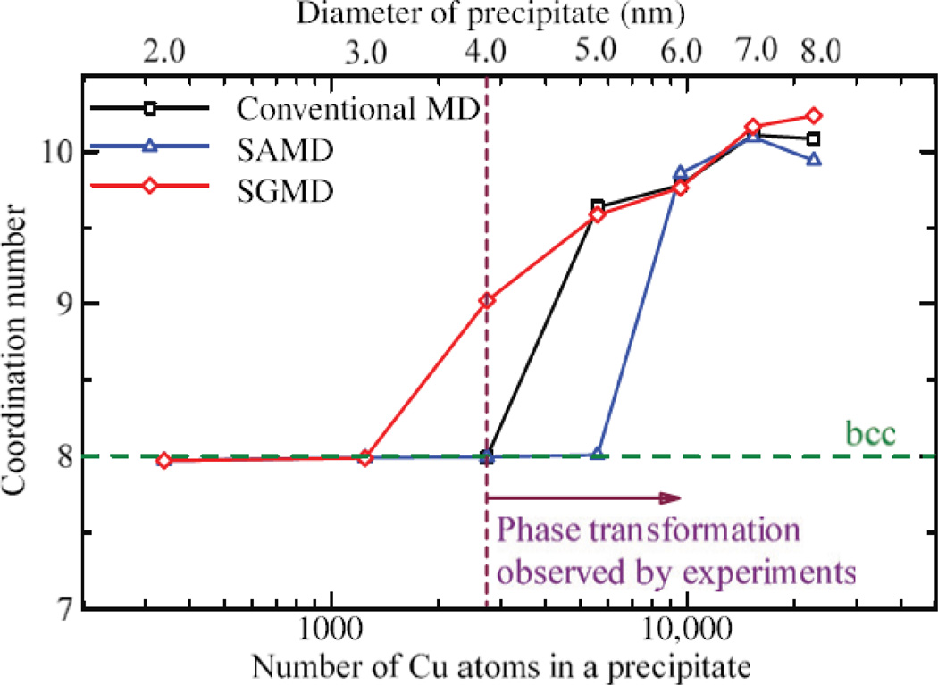
The self-guided molecular dynamics (SGMD) (Wu & Wang 1998; 1999) and the self-guided Langevin dynamics (SGLD) (Wu & Brooks 2003; Wu & Brooks 2011a; 2011b) simulation methods were developed for an efficient conformational search and have found many applications to study rare events, such as protein folding (Lee & Chang 2010; Lee & Olson 2010; Wen et al 2004; Wen & Luo 2004; Wu & Sung 1999; Wu & Brooks 2004; Wu & Wang 2000; 2001; Wu et al 2002), and ligand binding (Lung et al 2001; Varady et al 2002; Yang et al 2004), docking (Chandrasekaran et al 2009), conformational transitions (Damjanovic et al 2009; Damjanovic et al 2008a; Damjanovic et al 2008b; Pendse et al 2010), crystallization (Abe & Jitsukawa 2009; Choudhary & Clancy 2005a; 2005b; Tsuru et al 2010; Wu & Wang 1999), and surface absorption (Sheng et al 2010a; 2010b)
In this review, we provide a comprehensive picture of the SGLD method to explain why and how it works. We first present the history of the development of SGMD and SGLD methods. The theoretic basis as well as the simulation methods in a variety of forms is provided in a comprehensive way in the thermodynamics of SGMD/SGLD section. In the Characteristics of SGLD section through several simple systems we explain the reason why SGLD can enhance conformational search. In the Application section, we review the applications of SGMD and SGLD in computational studies up to date. And finally, in the Summary section we present the development direction and guidance in applying SGMD and SGLD methods.
History of the SGMD and SGLD methods
The idea of a self-guided simulation is to promote conformational transitions according to the information extracted during the same simulation in order to achieve faster convergence in conformational sampling. The information extracted during a simulation is called a local average property. The averaging is taken over the conformational space near the current conformation and can be approximately estimated by the following function:
| (2) |
Here L is the number of local conformations used for the averaging, P[n] is a conformational property at conformation n. The symbol < >L denotes a local average. The contribution of any conformation to a local average decays exponentially with a decay factor of L.
The local averaging was first utilized to estimate the mean solvation force in protein folding simulations with explicit solvent (Wu & Sung 1999). Explicit solvent molecules dampen protein motion and the conformational transition is slow. Furthermore, the noise from the solvent collisions is overwhelming; as a result, much of protein motion appears as a random walk. The mean force of the interaction with the solvent represents the solvation free energy force, which excludes the noise of solvent interaction and guides the protein to conformations favored by solvation. In this method the solvent environment is simulated with a Monte Carlo method, while the protein was simulated with molecular dynamics, the mean solvation force was replaced by the local average solvent interaction force and was calculated using eq. (2) with a local average size of L=10. The equation of motion for the protein can be written as:
where ṗi and fi are the time derivative of momentum and the interaction force of atom i in a protein, respectively. s̃i is the local average force of solvent on protein atom i.
The self-guided molecular dynamics (SGMD)(Wu & Wang 1998; 1999) simulation method was developed by extending the local average force to all atoms and by including all nonbonded forces.
Here gi is the guiding force, which is calculated as a local average of the non-bonded force:
| (3) |
The parameter, λ, is the guiding factor, δt is the time step, and tL = Lδt is the local averaging time. In an SGMD simulation, the system undergoes an accelerated systematic motion, which is defined by the local averaging time, tL, while maintaining a desired temperature. Many applications have demonstrated that SGMD simulations have an enhanced conformational search ability (Choudhary & Clancy 2005a; 2005b; Lung et al 2001; Sheng et al 2010a; 2010b; Varady et al 2002; Wu & Wang 2000; 2001; Wu et al 2002). Shinoda and Mikami extended SGMD to the NPT ensemble (Shinoda & Mikami 2001) and later combined it with the rigid body dynamics (Shinoda & Mikami 2003).
There are several drawbacks when applying the SGMD method. First, the guiding force calculated by eq. (3) is correlated with the force field and results in an unwanted alteration of the conformational distribution. Second, for molecular systems, high frequency bonded interactions need to be excluded in the guiding force calculation to avoid excessive noise. Third, as pointed by Lahiri et al. (Lahiri et al 2001), the guiding force derived from the local average of actual forces may not be sufficient to enhance conformational searching in stochastic dynamics simulations.
Andricioaei et al. extended the self-guiding idea to a hybrid Monte Carlo simulation method (MHMC) to enhance conformational sampling efficiency (Andricioaei et al 2003). They used the local average momentum as a guide to bias the initial choice of momenta at each step. They demonstrated that their self-guided enhanced sampling method enhances conformational sampling efficiency while producing, theoretically, correct thermodynamic average properties in the weak perturbation limit.
The local average momentum has some advantages over the local average force to be used as the guiding force. However, due to the correlation between the local average momentum and the instantaneous momentum, directly applying the guiding force of this type could make fast objects move faster and cause an uneven distribution of kinetic energy throughout the simulation system.
Langevin dynamics (LD) simulation has been a very useful tool in macromolecule studies (Allen & Tildesley 1987). It is also used as a temperature-control scheme to maintain constant temperature (Pastor et al 1988). Obviously, introducing a guiding force to accelerate the systematic motion can enhance conformational search efficiency of an LD simulation. Based on the position Langevin equation, we found that the guiding force can be represented by the local average of friction forces, which is proportional to the local average of momenta. Therefore, the guiding force takes the form of local average momentum in the self-guided Langevin dynamics (SGLD) method:
| (4) |
where γi is the collision frequency and Ri is a random force for particle i. The parameter, ξ, is an energy conservation parameter, which is set to cancel the extra energy input from the guiding forces.
The enhanced conformational searching ability of SGMD and SGLD are demonstrated by their many applications in protein folding (Lee & Chang 2010; Lee & Olson 2010; Wu & Wang 2000; 2001; Wu et al 2002), ligand binding (Lung et al 2001; Varady et al 2002; Yang et al 2004), conformational transitions (Damjanovic et al 2009; Damjanovic et al 2008a; Damjanovic et al 2008b; Pendse et al 2010), phase transitions (Abe & Jitsukawa 2009; Choudhary & Clancy 2002; Chowdhury et al 2003; Tsuru et al 2010; Wu & Wang 1999), and surface adsorption (Sheng et al 2010a; 2010b). There are several method developments along the same concept of SGLD. For example, Yang and Gao presented an approximate method to use a relative short normal dynamics simulation to obtain slow motion information to propagate structure changes in the slow degrees of freedom (Gao et al 2008; Yang & Gao 2007). Similarly, MacFadyen et al. proposed a method that utilizes a directional negative friction force to enhance sampling efficiency for rare events (MacFadyen et al 2008). However, there was lack of understanding why conformational search is accelerated and how the guiding forces affect conformational distribution. And the most practical question is how to obtain canonical conformational distribution with the accelerated conformational search techniques. These questions hindered the application of SGMD and SGLD in quantitative studies, such as free energy calculation.
Recently, a quantitative understanding of the perturbation on conformational distribution by the local average momentum based guiding force has been achieved (Wu & Brooks 2011b). The partition function in an SGLD ensemble is quantitatively related to the so called low frequency properties defined based on the local averaging scheme. Through the SGLD partition function, the conformational distribution obtained in SGLD simulations can be converted to a canonical ensemble distribution, and ensemble average properties can be calculated from SGLD simulations through reweighting. Because the energy distribution of an SGLD simulation is very close to the canonical distribution, the reweighting can be calculated with high accuracy for a large range of guiding factors. Another convenience is that the reweighting factor can be computed efficiently either on-the-fly or during post processing, which means that SGLD can be used to compute free energies in a direct manner without the need for post processing.
Based on the understanding of SGLD conformational distribution, an SGLD combined with SGMD simulation method (Wu & Wang 1998; 1999), called force-momentum based self-guided Langevin dynamics, or SGLDfp, has been developed, which utilize the force-based guiding force to cancel any conformational bias due to the momentum based guiding effect(Wu & Brooks 2011a). Through this combined guiding force we can accelerate conformational search while preserving canonical conformational distribution without the need for any reweighting. In other words, the method is explicitly designed so that every sampled conformation would have the same reweighting coefficient. The one drawback of SGLDfp is that it is not as efficient as SGLD with reweighting. As a rough rule of thumb, SGLD will cross barriers of 20 kT at the rate that LD or MD will cross barriers of 10 kT (an effective doubling of temperature), but SGLDfp only crosses barriers of 15 kT at the same rate. Details depend on systems and parameters used, so this is only a rough guide.
This progress in the understanding of the SGLD conformational distribution and conformational search and the development of the SGLDfp method open the door for numerous types of quantitative simulation studies.
Thermodynamics of SGMD and SGLD
The low-frequency and high-frequency properties
Thermal motion in a molecular system has a wide distribution of frequencies. Chemical bonds vibrate and bend at high frequencies, while ion transport and protein folding events occur on a relatively long time. High frequency events repeat on a short time scale and are often the easiest to study in molecular simulations. Low frequency events are important for many macroscopic behaviors such as protein folding, binding, and conformational rearrangements, but are often beyond the time scale accessible by molecular simulations with available computing resources.
Low frequency properties are related to low frequency events. For example, dimerization of a pair of water molecules depends on the relative position between the water molecules. This dimer energy means the energy when the two water molecules at the dimer state, i.e., the average among all bond vibration and bending states. This dimer energy represents the energy at a frequency of dimerization, which is a slow event as compared to bond vibration and bending. At each given moment, bond vibration and bending, and even electron density fluctuations, produce an instantaneous energy deviation, which depends on the high frequency motions. The energy associated with such high frequency motions is called high frequency energy. Compared with the bond vibration and bending, dimer energy is a low frequency energy, which is an average over all the vibration and bending states. For slow events, low frequency properties give a more accurate picture, while for fast events, high frequency properties are needed to describe them.
We propose to define a low frequency property by the so called local average property. A local averaging procedure involving an exponential decay average(Wu & Sung 1999; Wu & Brooks 2003; Wu & Wang 1998; 1999), typically on force or momentum, is performed by the following equation:
| (5) |
Here, P[i] represents property P at the ith data point and P(t) represents the one at time t. As can be seen from eq. (5), a local average, denoted as “< >L”, is calculated by averaging over the most recent L points, or the most recent tL = Lδt time period. Here, δt is the time interval between data points. We call L the local averaging size and tL the local averaging time. This average can be approximately calculated as an evolving average with a constantly updating of current value as shown in the right hand portion of eq. (5). This evolving average is denoted with a “~” cap: P̃. Because all local averages in this work are calculated as evolving averages, we also use “< P >L” to represent evolving averages when the cap “~” is not easy to print. Corresponding to the low frequency properties, we define high frequency properties as the difference between instantaneous properties and their low frequency ones: P − P̃. Both the low frequency and high frequency properties are conformational dependent or time dependent, and can be expressed as functions of time: P̃(t) and P(t) − P̃(t), in molecular dynamics simulation.
The local averaging shown in eq. (5) suppresses high frequency effects and emphasizes low frequency contributions. From eq. (5) we can see that the local average time, tL, determines the contribution frequency range. To better understand the evolving averaging, we can rearrange eq. (5) to the following form:
When δt →0, we have:
This differential equation can be solved:
| (6) |
Therefore, a property at any moment provides an exponentially decaying contribution to the evolving average as a function of time. The decaying rate depends on the local average time, tL.
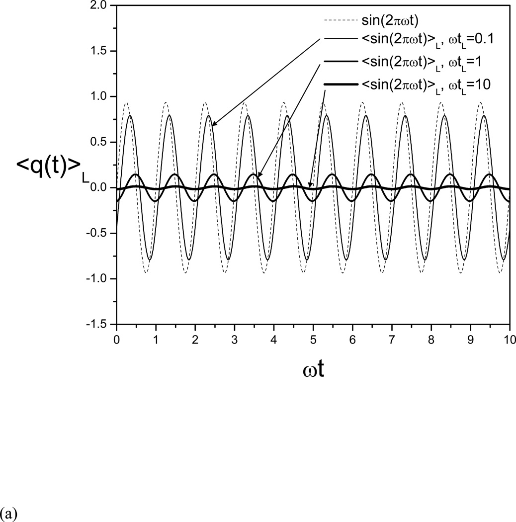
The separation of the low frequency properties and the high frequency properties is at the heart of the SGLD simulation method. The low frequency properties are calculated through the evolving averaging shown in eq. (5). To explain the behavior of the evolving averaging, we use q(t) = sin(2πϖt) as an example function of frequency ϖ to show how frequency and local average time affect the evolving average.
Substituting q(t) = sin(2πϖt) into eq. (6), we get its evolving average:
| (7) |
As can be seen from eq. (7) that for high frequency, 2πϖtL >> 1, the amplitude of q̃(t) is inversely proportional to ϖ, while for low frequency, 2πϖtL << 1, q̃(t) ≈ q(t). The local average time, tL, defines the separation of what is high frequency and what is low frequency as compared with a local averaging frequency of . This example shows that the evolving averaging suppresses the high frequency contribution while has less effect on low frequency components. The high frequency portion can be expressed as:
| (8) |
As can be seen from eq. (8), when 2πϖtL >> 1, q(t) − q̃(t) ≈ sin(2πϖt) = q(t), and when 2πϖtL << 1, q(t) − q̃(t) ≈ −2πϖtL(e−t/tL − cos(2πϖt)) → 0. That is, the high frequency portion keeps the high frequency contributions while suppressing the low frequency components.
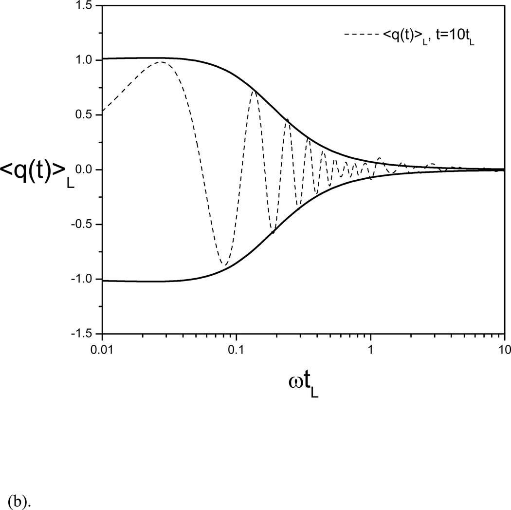
Fig. 1(a) shows the example function and its evolving averages at different local average times. Clearly, one can see that the frequencies of the averaging results remain the same as the example function, but the amplitudes and phases are very different from each other. When ϖtL = 0.1, this function represents a low frequency motion and its evolving average has a magnitude similar to the function. When ϖtL = 10, this function represents a high frequency motion and the magnitude of its evolving average is very small compared to the function. Fig. 1(b) shows an averaging result as an function of ϖtL. The envelop function represents the amplitude of the averages. Clearly one can see, with a small ϖtL, the amplitude of the average is similar to the example function, while with a large ϖtL, the amplitude of the average approaches zero, indicating that the low frequency function will remain in the evolving average and the high frequency function will be suppressed.
Fig. 1.
(a) The example function, q(t) = sin(2πϖt), and its evolving averages at three local average times: ϖtL = 0.1, 1, and 10.
(b) The evolving average of the example function as a function of the frequency. The envelope curves show the amplitude as a function of ϖtL. At small ϖtL, which corresponds to a low frequency, the amplitude is approaching 1, very similar to that of the example function, while at a large ϖtL, which corresponds to a high frequency, the amplitude approaches 0.
In summary, conformational properties can be separated into high frequency and low frequency properties based on the local averaging time, tL. Through the local averaging, many low frequency properties can be obtained in molecular simulation. For example, low frequency forces:
low frequency momenta:
and low frequency potential energies:
| (9) |
We can calculate some derived low frequency quantities from these low frequency properties, such as the low frequency temperature:
| (10) |
Here, NDF is the number of degrees of freedom and k is the Boltzmann constant. mi is the mass of particle i and the summation runs over all atoms in a system. The bracket, 〈 〉, represents an ensemble average.
SGMD and SGLD simulation methods
Because molecular dynamics can be regarded as a special case of Langevin dynamics, to be general, we give the following description and explanation based on the self-guided Langevin dynamics. The equation of the self-guided motion can be written in the following general form:
| (11) |
where ṗi and fi are the time derivative of momentum and the interaction force of particle i, respectively. Ri is a random force, which is related to mass, mi, the collision frequency, γi, and simulation temperature, T, by the following equation:
| (12) |
gi is called the guiding force and is calculated based on the low frequency momentum or the low frequency force, or both. Even though eq. (11) is in the form of the self-guided Langevin dynamics, it can represent an SGMD motion when the collision frequency, γi, and the random force, Ri, are zero. From eq. (11) we can see that molecular dynamics and Langevin dynamics are special cases of SGLD when the guiding force is zero and/or the collision frequency is zero. Depending on how the guiding force is calculated, eq. (11) can represent different kinds of self-guided dynamics motion. For example, SGMD calculates the guiding force with nonbonded forces (Wu & Wang 1998; 1999), SGLD uses momentum (Wu & Brooks 2003) and is also referred to as SGLDp, and SGLDfp uses both forces and momenta (Wu & Brooks 2011a). As a summary, Table I lists the derivative forms of SGLD and their guiding forces. So far, SGMD, SGLD, and SGLDfp have been well documented while SGMDf, SGMDp, SGLDf, and SGMDfp have not been studied.
Table I.
The guiding forces used in self-guiding molecular dynamics and self-guided Langevin dynamics in a variety of derivative forms
| Name | Parameters | Guiding force1 | |
|---|---|---|---|
| SGMD (Wu & Wang 1998; 1999) 2 | λf, tL |
|
|
| SGMDf | λf, tL |
|
|
| SGMDp3 | , tL |
|
|
| SGMDfp4 | , tL |
|
|
| SGLD or SGLDp (Wu & Brooks 2003) (Wu & Brooks 2011b) | , tL, γi | ||
| SGLDf | λf, tL, γi | ||
| SGLDfp (Wu & Brooks 2011a) | , tL, γi |
the parameter, ξp, is an energy conservation factor to cancel the energy input from the guiding force and can be calculated by: . γ0 = 1/ps is a force converting factor.
In SGMD, only nonbonded forces, , are used to calculated the guiding force.
SGMDp is SGLD with γi = 0.
SGMDfp is SGLDfp with γi = 0.
Conformational distribution in SGLD
The guiding force in an SGLD simulation is designed to accelerate the low frequency motion so that the conformational search efficiency can be enhanced. It has two types of effects on a simulation system. First, the guiding force enhances low frequency motion as measured by the increase in the low frequency temperature, and it also reduces the high frequency motion due to the energy conservation force that comes with the guiding force. Second, the guiding force produces a bias in the energy surface. To understand the conformational distribution in SGLD simulation, we separately examine the low frequency motion and high frequency motion.
In the low frequency conformational space, the equation of motion can be expressed as a low frequency portion of eq. (11):
| (13) |
The low frequency motion is on the low frequency potential energy surface, Ẽp, under the low frequency interaction force, f̃i, and the low frequency guiding force, g̃i, the low frequency friction force, γip̃i, and the low frequency random force, R̃i. Based on the “position Langevin equation”, the momentum, as well as the momentum based guiding force, are correlated with the interaction force (Wu & Brooks 2003). Therefore, the total low frequency force, f̃i + g̃i − γip̃i + R̃i, acts as a force from a scaled low frequency potential energy surface, Elf = λlfẼp. The low frequency energy factor, λlf, can be approximated according to the average projection of the total low frequency force in the direction of the low frequency interaction forces:
| (14) |
Beside the scaling effect in the low frequency potential energy, the guiding force also enhances the low frequency motion. This enhanced low frequency motion corresponds to an elevated thermal temperature in the low frequency conformational space. We define this thermal temperature in the low frequency conformational space as Tlf. It is reasonable to assume that Tlf is proportional to the low frequency temperature, T̃:
| (15) |
Here, T̃0 is the low frequency temperature when λ = 0 and is called the reference low frequency temperature. Based on the definition, we know T̃0 depends on the simulation condition and the local average time, tL.
To understand the relationship between T̃ and T̃0, we can rewrite the low frequency motion, eq. (11), to a Langevin dynamics form:
| (16) |
eq. (16) corresponds to a Langevin dynamics with a collision frequency of χlfγi. The factor, χlf, is called the low frequency collision factor and can be calculated according to the projection of the low frequency guiding force in the direction of the low frequency friction force:
| (17) |
Based on the Langevin dynamics relation, eq (12), with a given distribution of random forces, the product of temperature and collision frequency is a constant:
| (18) |
The reference low frequency temperature, T̃0, corresponds to the low frequency temperature at a collision frequency of γi, while the low frequency temperature in an SGLD simulation, T̃, corresponds to that at the collision frequency of χlfγi. Because the guiding force does not affect the random force, from eq. (18) we have
| (19) |
Eq. (19) provides a relationship among χlf, T̃0, and T̃. We can calculate χlf either from Eq. (16) or from Eq. (19) with , which is more accurate if T̃0 has been obtained from a previous SGLD simulation with λ = 0.
Combining the scaling in the low frequency potential energy surface and the elevation in the low frequency motion, we have the partition function in the low frequency conformational space:
| (20) |
Similarly, in the high frequency conformational space, the equation of motion can be expressed as the difference between the instantaneous motion, eq. (11), and the low frequency motion eq. (13):
| (21) |
The potential energy surface is approximated as the scaled high frequency potential energy surface, Ehf = λhf(Ep − Ẽp). The high frequency energy factor, λhf, is calculated as the average projection of the total high frequency force in the direction of the high frequency interaction force:
| (22) |
Again, we define the effective thermal temperature in the high frequency conformational space as Thf and assume Thf is proportional to the high frequency temperature, T − T̃:
| (23) |
Similarly, we can calculate the high frequency collision factor:
| (24) |
Combining the scaling in the high frequency potential energy surface and the repression of the high frequency motion, we have the partition function in the high frequency conformational space:
| (25) |
The overall partition function of an SGLD ensemble is the product of that in the low frequency and the high frequency conformational spaces:
| (26) |
In summary, at a given temperature, T, the guiding force produces the following effects in both low and high frequency conformational spaces:
In the low frequency conformational space, the low frequency energy surface, Ẽp, is modified by a factor of λlf. The effective temperature is changed from T to .
In the high frequency conformational space, the high frequency energy surface, Ep − Ẽp, is modified by a factor of λhf. The effective temperature is changed from T to .
The partition function of a canonical ensemble from an LD simulation can be related to that of an SGLD ensemble by the following equation:
| (27) |
Here, wSGLD is called the SGLD reweighting factor:
| (28) |
Any ensemble average, <P>, can be calculated in an SGLD simulation as:
| (29) |
Because SGLD simulation does not change temperature, the average energy contribution to the reweighting factor can be removed:
| (28’) |
As can be seen from Eq. (28'), the reweighting factor, , depends on the energy change, instead of the total energy, and can be calculated much more easily numerically than wSGLD. The factors, λlf, λhf, χlf, and χhf, are all around 1. Therefore, is actually used in place of wSGLD for reweighting calculation, Eq. (29). The reweighting factor of SGLD simulations has relatively narrower value range than other approaches such as with high temperature simulations, which enable accurate reweighting calculation in SGLD simulations. The SGLD reweighting factor can be calculated on-the-fly during an SGLD simulation to avoid a post-processing of a simulation trajectory.
Conformational search in SGLD
In SGLD simulations, the guiding factor, λ, is a unitless input parameter whose value is often hard to decide for its lack of physical meaning. For convenience in describing the conformational search ability of an SGLD simulation, we define a self-guiding temperature, Tsg, based on the effective temperatures in the low and high frequency conformational spaces:
| (30) |
The self-guiding temperature, Tsg, provides a rough measure of the conformational searching ability in the unit of temperature. An SGLD simulation with a self-guiding temperature of Tsg has a conformational search ability comparable to that in a high temperature simulation at the temperature of Tsg. As can be seen from eq. (30), for an LD simulation, T̃ = T̃0, we have Tsg = T. For an SGLD simulation with λ>0, we have T̃ > T̃0 and Tsg > T, and with λ<0,, we have T̃ < T̃0 and Tsg < T. Tsg can be used as a guidance for the choose of λ. For example, it is reasonable to choose a λ that produces Tsg = 2T. However, when λ is large and Tsg is too large as compared to T, it is difficult to obtain accurate canonical ensemble through reweighting with eq. (25) and eq. (26). Therefore, λ should be chosen to balance the acceleration of conformational search and the accuracy in converting the conformational distribution.
Force-momentum based self-guided Langevin dynamics (SGLDfp) simulation method
SGMD utilizes the local average forces while SGLD uses the local average momentum to calculate the guiding force to achieve accelerated conformational search. These two types of guiding forces have opposite bias effect on the low frequency energy surface. The low frequency force, f̃i, favors low Ẽp states, just as normal forces do, while the low frequency momentum, p̃i, favors high Ẽp states, just as high temperature does. These two types of low frequency properties can be combined in such a way to have the bias effects cancelled.
Let’s define a guiding force, gi, as a linear combination of f̃i and p̃i in the following form:
| (31) |
Here, λf is the force guiding factor and ξf is the force damping factor. The energy conservation factor, ξp, is calculated by the following equation to cancel the energy input from the guiding force at every time step:
| (29) |
The low frequency energy factor is now:
| (32) |
The high frequency energy factor is:
| (33) |
Here, we use and to represent the momentum based energy factors calculated using Eq. (13) and Eq. (22). and , as well as χlf, and χhf, are calculated during simulations as accumulating averages (Wu & Brooks 2011a). We can set λf and ξf during a simulation in such a way:
| (34) |
and
| (35) |
so that
| (36) |
| (37) |
and we have:
| (38) |
From above equations, we can see that by using a guiding force with a balanced local average force components as shown in Eqs. (34) and (35) we can directly obtain an unbiased conformational distribution. Therefore, an ensemble average property can be directly calculated from an SGLDfp simulation:
With such a direct approach, the sampled conformation can be directly used for computing ensemble averages, such as free energy. As such, SGLDfp equation of motion can directly replace MD or LD for any non-driven degree of freedom in a rather unbiased manner. For example, the generalized ensemble (GE) methods (Li et al 2007a; Min & Yang 2008; Zheng et al 2009) are enabled via the free energy flattening (or effectively flattening) treatment. Therefore, these methods intrinsically suffer from the diffusion sampling problem (Li et al 2007; Min & Yang 2008). Complementary to the GE strategy, SGLD or SGLDfp improves the sampling by improving local diffusion. One can naturally expect that the combination of the SGLD or SGLDfp method and the efficient GE method such as OSRW will lead to significant sampling improvement; this expectation should be especially true when the collective variables associated with large number of degrees of freedom such as essential energy (Li et al 2007; Zheng & Yang 2008) or generalized force (Min et al 2011; Zheng et al 2009) are employed.
Details of the simulation algorithms of SGMD (Shinoda & Mikami 2001; 2003; Wu & Wang 1998; 1999), SGLD (Wu & Brooks 2003; Wu & Brooks 2011b), and SGLDfp (Wu & Brooks 2011a) have been reported previously. SGLD is available in CHARMM (Brooks et al 2009; Brooks et al 1983) version 32 and later. SGLD reweighting and SGLDfp have been implemented into CHARMM version 36. Because SGLD and SGLDfp simulations involve extra calculation only in the propagation of the equation of motion as compared to normal LD simulation, the cost of SGLD and SGLDfp simulation is almost identical to an LD simulation for the same number of time steps. SGLD and SGLDfp simulations do keep more arrays in memory because of the need to store the guiding forces, as well as some arrays for the weighting factor calculation.
To run an SGLD or SGLDfp simulation, one can either set λ (or for SGLDfp) or set a target self-guiding temperature, , defined by eq. (30). When is set, is adjusted in such a way:
| (39) |
so that Tsg will approach . λf and ξf will be calculated according to Eqs. (34) and (35) the same way as when is set. Because Tsg is a derived quantity, its value range is limited by the simulation temperature, system size, and other SGLD parameters, must be set close to the simulation temperature to produce a converged . For example, one may set for an SGLDfp simulation. To achieve an optimal performance, it may be necessary to briefly explore various SGLD parameters to find an optimal set of parameters for a particular system.
Characteristics of the self-guided Langevin dynamics
We use several model systems to demonstrate the nature and to explain the characteristics of SGLD simulations. The model systems we choose are a skewed double well system, argon liquid, an alanine dipeptide, and a pentamer peptide. Through these model systems, we demonstrate the effect of the guiding force on kinetic energy and potential energy distributions, low frequency motion and high frequency motion, as well as energy barrier crossing ability. In addition, we examine how the low and high frequency properties changes with the guiding factor λ, and the local averaging time, tL, as well as the collision frequency, γ. Because only is set and is the same for all particles, in the following description the guiding factor, λ, refers to the momentum guiding factor, .
The skewed double well system
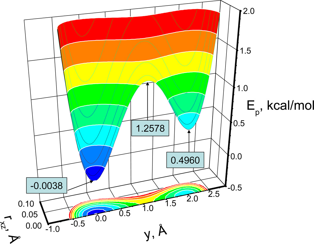
A skewed double well system represents the simplest system with an energy barrier to cross. This system has only one particle and the particle moves on a fixed energy surface. The skewed double well potential energy (in kcal/mol) has the following form:
| (40) |
Fig. 2 shows the energy surface of this double well potential. This energy surface is designed in such a way that it restricts the particle to move near the y-axis with two energy minima of different depths, −0.0038 kcal/mol and 0.4960 kcal/mol, along the y-axis at (0, −0.0299, 0) and (0, 1.9672, 0), respectively. The potential is symmetric around y-axis with a strong dependence on the distance from y-axis, . The minimum transition energy from one well to the other well is 1.2578 kcal/mol at (0, 1.0627, 0) between the two wells. Such a design forces the particle to have a high frequency motion in the x-z direction and a low frequency motion in the y direction.
Fig. 2.
The energy surface of the skewed double well potential. The potential is symmetric around the y–axis and is the distance to the y-axis.
An argon atom was used to represent the particle. Simulations were carried out with a local averaging time, tL=0.2 ps. A time step of 1 fs was used and the simulation length was 1 µs for each simulation. The collision frequency was 10/ps except noted otherwise. To help illustrating the guiding force effect, we used a large range of the guiding factor, up to λ=2.
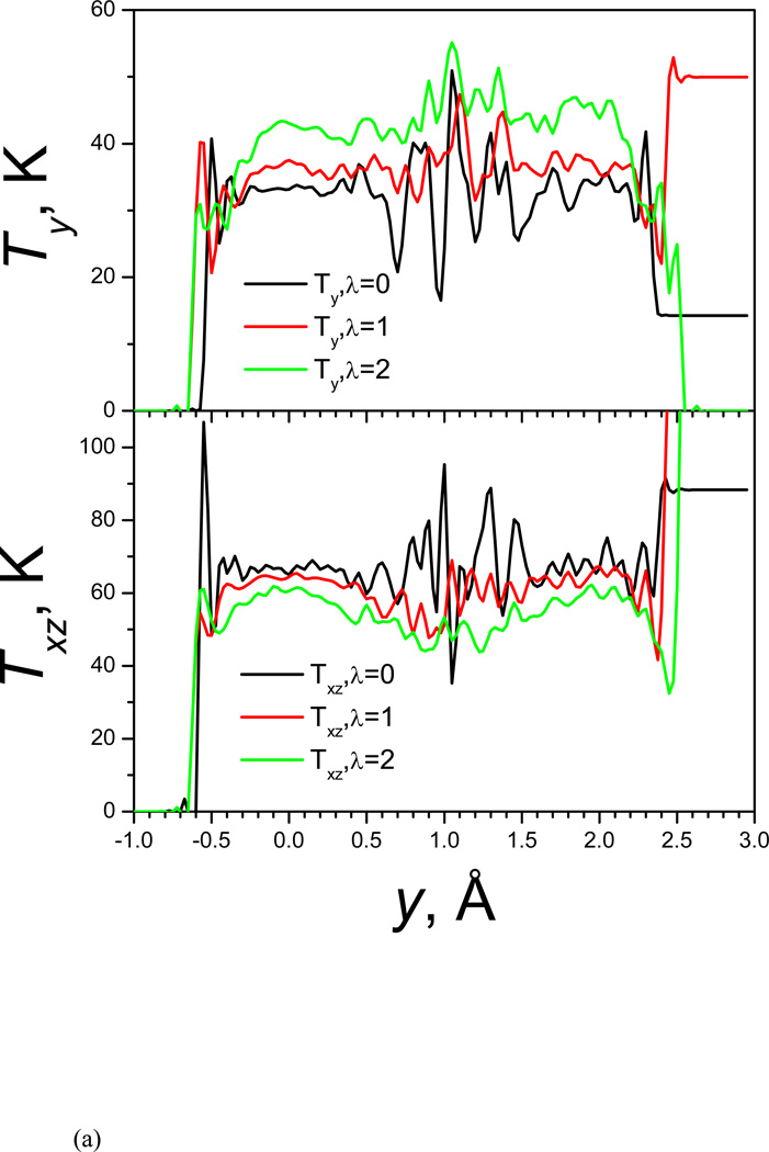
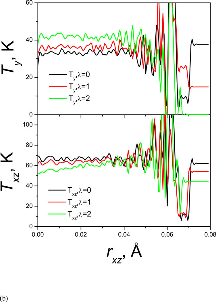
Kinetic energy is transferred from high frequency degrees to low frequency degrees. This double well system has only three degrees of freedom in x, y, and z directions. In the y direction the atom has low frequency motion while in the x and z directions it has high frequency motion. We calculate the temperature components based on its velocity components to examine the kinetic energy changes with the guiding force. Fig. 3(a) and Fig. 3(b) show the kinetic energies in the low frequency direction (along the y-axis) and in the high frequency direction (perpendicular to the y-axis, or along the x-z plan) as function of y and rxz, respectively. The top and bottom panels of Fig. 3(a) show the y and x-z component of temperature as functions of the y coordinate. At λ=0, Ty and Txz are almost constant throughout the accessible y coordinate range. Large fluctuations are observed around the energy barrier around y=1 Å due to the poor sampling in this region. As λ increases, Ty increases, while Txz decreases. The changes in Ty and Txz are not uniform. Larger changes can be seen in the energy barrier region than in the well regions. This result explains why the guiding force helps energy barrier crossing. The guiding force pumps kinetic energy from high frequency degrees of freedom to low frequency degrees of freedom to overcome energy barrier, and the higher the energy barrier, the more kinetic energy is transferred. The kinectic energy transfer can also be seen in Fig. 3(b) in the x-z coordinate range, but in this high frequency coordinate range, more kinetic energy transfer is observed in low energy region (smaller rxz). Once the barrier is crossed, the excess kinetic energy in the low frequency motion is returned to the high frequency degrees of freedom in a non-thermostat manner. The overall effect can be though as “energy borrowing”.
Fig. 3.
(a)Temperature in y-coordinates; (b) temperature in rxz.
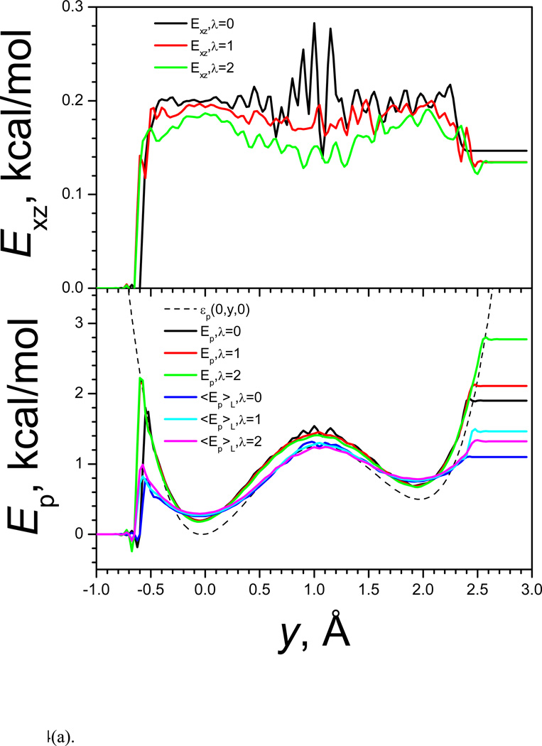
The guiding force favors low potential energy region in the high frequency degrees of freedom and high potential energy in the low frequency degrees of freedom. Fig. 4 shows the average potential energy and its components as functions of the coordinates. Fig. 4(a) shows the energies along the y coordinates. The top panel of Fig. 4(a) shows the x-z component the total energy, Exz, which represents the high frequency portion. In LD simulation (λ=0), Exz is almost flat throughout the accessible y coordinate range except a large fluctuation around the barrier region (around y=1) due to poor sampling. When λ increases, Exz decreases and decreases more at the energy barrier region. The fluctuation in the energy barrier region becomes much smaller because of the improved sampling in the SGLD simulation. The bottom panel of Fig. 4(a) shows the y component, Ey = εy (y) = εp (0, y, 0), and the total potential energy, Ep, as well as the low frequency potential energy, Ẽp. The total potential energy is the sum of the y component and the x-z component shown in the top panel: Ep = Exz + Ey. Ey depends only on the y coordinate and will not change with λ. Even though, we can see from Fig. 4(a) that the accessible y range increases with λ, indicating higher energy states are reached with larger λ.
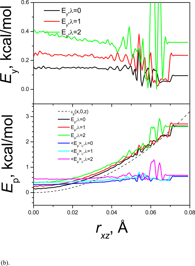
Fig. 4.
(a) Average potential energies in y-coordinates; (b) average potential energies in x-z direction.
Comparing Ep and Ẽp in Fig. 4(a), we can see that Ẽp has smaller energy barrier than Ep. Low frequency energy surface tends to have lower energy barriers. In other words, the low frequency energy surface is smoother than the original energy surface. Enhanced motion in the low frequency energy surface can be more efficient to cross energy barrier than to do that in the original energy surface.
Fig. 4(b) shows the average potential energy and its components at different rxz. From the top panel of Fig. 4(b) we can see that in LD simulation (λ=0), Ey is almost flat and in SGLD simulations, Ey increases with λ and increases more in smaller rxz. The lower panel of Fig. 4(b) shows that Ẽp is almost flat, indicating the high frequency energies are averaged out in the local averaging process.
Overall, the guiding force accelerates the low frequency motion while slows down the high frequency motion. As a result, the simulation has enhanced ability to overcome energy barriers in the low frequency conformational space while making high frequency states more stable. These features contrast SGLD against high temperature simulations. SGLD can preserve high frequency structures while enhancing conformational search in the low frequency conformational space. High temperature simulation will destabilize all structures.
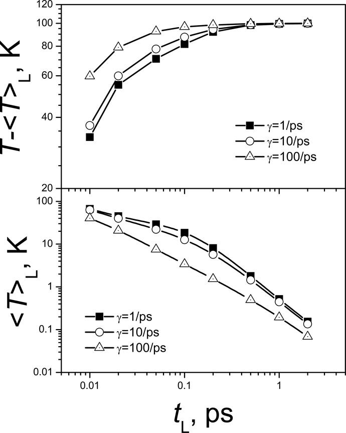
Another important parameter for SGLD simulations is the local averaging time, tL. It is used to define the low frequency property and the high frequency property through the evolving averaging, Eq. (5). The choice of tL will affect which motion will be enhanced and which motion will be suppressed. A larger tL will result in more motion falling into the high frequency motion category and less into the low frequency motion category, which is demonstrated in Fig. 5. The low frequency temperature, T̃, accounts for the kinetic energy of the low frequency motion. As tL increases, T̃ decreases (lower panel of Fig. 5), while the high frequency temperature, T − T̃, increases (top panel of Fig. 5). Low frequency temperature decreases with the collision frequency. Fig. 5 also shows the effect of collision frequency. As γ increases, T̃ decreases. This is because an increase in γ will increase the friction force, which will suppress more low frequency motion than high frequency motion.
Fig. 5.
The low frequency and high frequency temperatures at different local average time.
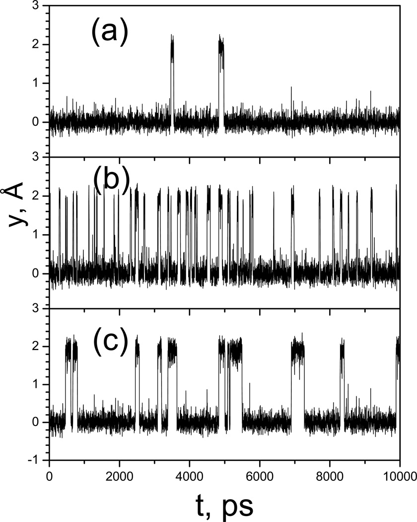
Now let’s examine the conformational search ability of SGLD and SGLDfp simulations. Fig. 6 shows the trajectories of the particle in the LD, SGLD, and SGLDfp simulations. Both the SGLD and SGLDfp simulations were run with λ=1. Clearly, both the SGLD and SGLDfp simulations increased transition rates as compared with the LD simulation. However, the SGLDfp simulation shows fewer transitions than the SGLD simulation due to the inclusion of a force-based guiding force to preserve the canonical ensemble.
Fig. 6.
Trajectories the particle on the double well potential. (a) LD simulation; (b) SGLD simulation with λ=1. (c) SGLDfp simulation with λ=1. The collision frequency is 10/ps and temperature is 80 K.
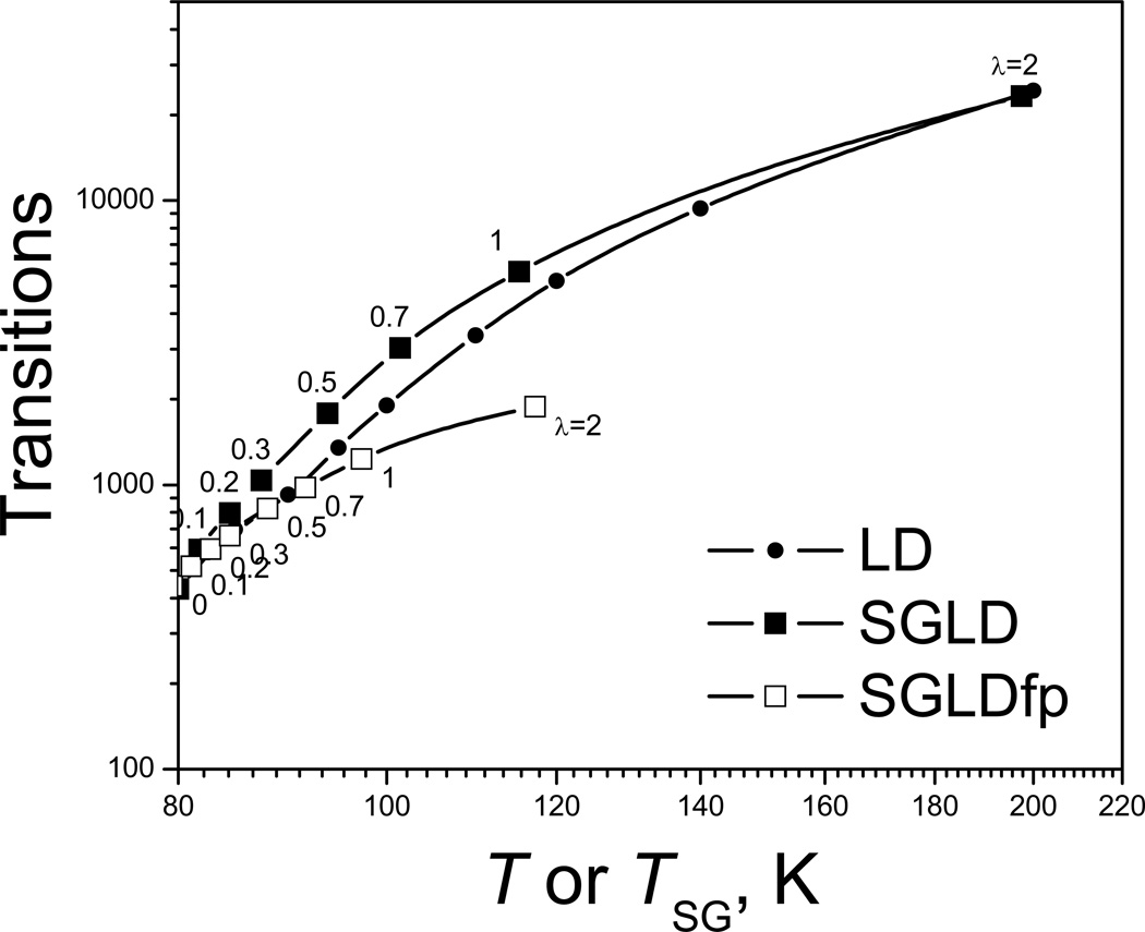
The self-guiding temperature, Tsg, is defined to describe the conformational search ability (Wu & Brooks 2011b). Fig. 7 compares the transition rate in high temperature LD simulations as a function of temperature and in SGLD or SGLDfp simulations as a function of Tsg. The guiding factor, λ, is labeled for each data point of the SGLD and SGLDfp simulations. The transition rate increases with T in the LD simulations and increases with Tsg in the SGLD or SGLDfp simulations. Even though the curves show different change rates with T or Tsg, they demonstrate that Tsg in the SGLD or SGLDfp simulations roughly reflect the transition rate of the LD simulations with T ≈ Tsg, especially when λ is small. The purpose of introducing Tsg is to provide a measurement of conformational search ability with certain physical meaning. It should be noted that an LD simulation at T ≈ Tsg is very different from an SGLD or SGLDfp simulation with a self-guiding temperature of Tsg. The major difference is that SGLD and SGLDfp simulations are performed at a temperature of interest which normally is lower than Tsg. The conformational distribution and energy distribution of SGLD simulations are very much closer to that of LD simulations at the same temperature rather than a high temperature where LD at T ≈ Tsg, while the distributions of SGLDfp simulations are the same as that of LD simulations at the lower temperature.
Fig. 7.
Transitions of the particle on the double well potential in high temperature LD simulations and in SGLD or SGLDfp simulations. x-axis is T for the LD simulations and is the self-guiding temperature, Tsg, for the SGLD or SGLDfp simulations. The guiding factors are labeled in the plot and the temperature is 80 K for the SGLD or SGLDfp simulations. The collision frequency is 10/ps and the transition count starts with 1. The simulation length is 1000 ns.
From Fig. 7 we can see the difference between the SGLD and SGLDfp simulations. In these simulations, the transition rates in both SGLD and SGLDfp simulations increase with Tsg, which depends on λ. At the same λ, an SGLD simulation has higher Tsg then an SGLDfp simulation. Even at the same Tsg, SGLD simulation has a higher transition rate. In the SGLD simulation with λ=1, the transition rate is about 13 times that of the LD simulation (i.e., λ=0). However, in the SGLDfp simulation with λ=1, the transition rate is only 2.9 times the LD rate. SGLDfp shows a reduced enhancement in energy barrier crossing as compared to the SGLD simulations, especially when λ is large. Therefore, the preservation of conformational distribution without reweighting comes at a cost of the reduced enhancement in conformational searching.
The collision frequency, γ, in Langevin dynamics plays an important role in representing a thermostatic environment. Through this skewed double well system, we can examine its effect on SGLD and SGLDfp simulations.
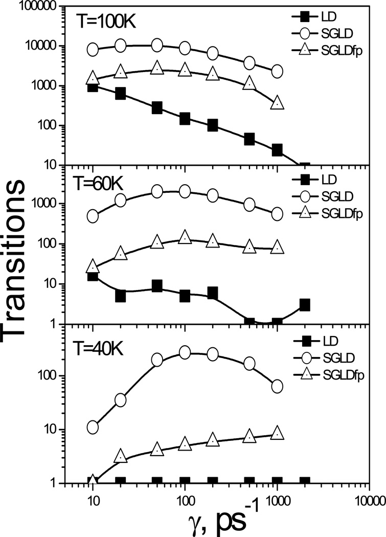
We performed a series SGLD and SGLDfp simulations with λ=1 at various γ and T, and the transition rates are shown in Fig. 8. The collision frequency controls the diffusion and the temperature corresponds to relative energy barrier heights. At T=100 K, 60 K, and 40 K, the average y-energies are 0.152, 0.0793, and 0.0561 kcal/mol, respectively. In kT scale, the energy differences between the global minimum and the transition barrier are 6.35 kT, 10.58 kT, and 15.87 kT, and the relative barrier heights from the average y-energies to the transition barrier are 5.56 kT, 9.89 kT, and 15.1 kT at T=100 K, 60 K, and 40 K, respectively.
Fig. 8.
Transitions of the particle on the skewed double well potential at different collision frequencies and temperatures. A guiding factor of λ=1 was used for all simulations. The transition count starts with 1. The simulation length is 1000 ns. The energy barrier heights from the y-average energies are (a) 5.56 kT at T=100 K; (b) 9.89 kT at T=60 K; and (c) 15.1 kT at T=40 K.
In Fig. 8 we can see that the transition rates of LD simulations decrease with γ at all temperatures. For the convenience of plotting, the transition count starts with 1. A transition value of 1 means the particle has never crossed the energy barrier. As can be seen in Fig. 8, at 40 K, LD cannot overcome the energy barrier in the simulation length even with a collision frequency of 10/ps. Higher γ reduces diffusion and slows down all events in LD simulations, regardless of their energy barriers. The transition rates of both the SGLD and SGLDfp simulations are higher than those in the LD simulations, demonstrating that SGLD and SGLDfp can enhance the barrier crossing and diffusion. The difference between SGLD and LD or between SGLDfp and LD increases as γ increases, indicating that the larger the friction force, the more acceleration the SGLD and SGLDfp will have. Comparing the SGLD and SGLDfp simulations, we can see the SGLDfp simulations have much fewer transitions than the SGLD simulations. This result indicates SGLDfp sacrifices the enhancement in conformational search to maintain correct conformational distribution. When γ approaches zero, the low frequency force and the low frequency momentum becomes highly correlated and the guiding effect approaches zero in the SGLDfp simulations. As can be seen from Fig. 8, the SGLDfp simulations have similar transition rates as the LD simulations when γ is small. This result means that SGLDfp performs better at larger γ.
In Fig. 8 there is a maximum in the transition rate at each temperature in the SGLD and SGLDfp simulations. Before the maximum collision frequency, γmax, the transition rate increases with γ and after that the transition rate decreases with γ. This is because as γ increases, the guiding force increases and the low frequency motion is enhanced. An increase in low frequency motion, combined with the increase in γ, will lead to an increase in friction forces. At γmax, the guiding effect is balanced by the friction effect. When γ > γmax, the slow down effect by the friction force surpasses the guiding effect and brings the transition rate down.
The value of γmax depends on the energy barrier. A higher energy barrier will result in a larger γmax. Comparing the transitions at different temperatures, γmax shifts up when temperature decreases. For SGLD simulations, at 100 K, γmax is between 20/ps and 50/ps, while at 60 K, γmax is between 50/ps and 100/ps, and at 40 K, γmax is between 100/ps and 200/ps. At lower temperature, energy barrier becomes a more dominant factor for the transition and the low frequency motion is slower, that makes γmax larger before the guiding effect is balanced by the friction force. Also, we can see in Fig. 8 that in the SGLDfp simulations, γmax are always higher than in the SGLD simulations. This is because SGLDfp has less energy barrier crossing ability than SGLD, which delays the maximum collision frequency where the guiding effect is balanced by the friction effect. Fig. 12 also demonstrates that SGLD and SGLDfp can overcome energy barriers as high as 15 kT (at 40 K) with reasonable transition rates where no LD transition is observed. Even at 30 K (corresponding to an energy barrier of 20 kT) we observed up to a hundred transitions in the SGLD simulations (data not shown).
Fig. 12.
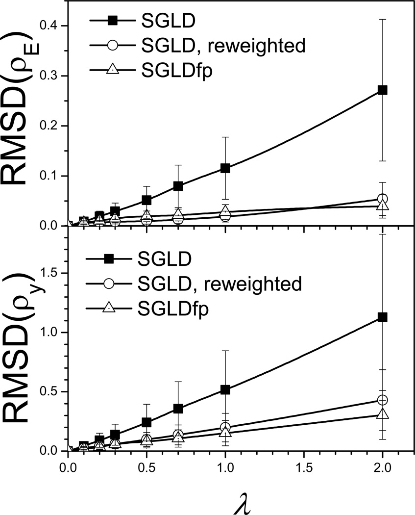
Root-mean-square deviations of the SGLD and SGLDfp distributions from the LD distributions. The upper panel shows the deviations in the potential energy distributions (kcal/mol) from Fig. 10 and the lower panel shows the deviations in the y-distributions from Fig. 11.
For macromolecular systems with a wide variety of barrier heights, a consensus value of γ needs to be used. Within CHARMM, different γ values can be applied to each atom, so that each part of a macromolecular system can be optimally enhanced. For example, the γ parameters that maximize the diffusion constant of water are different then those that maximally enhance protein side-chain transitions.
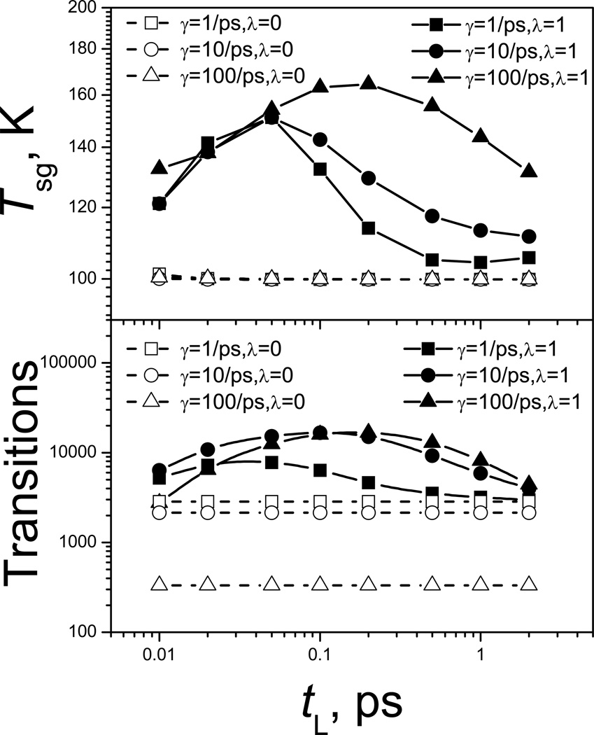
Fig. 9 shows the conformational search ability as measured by the self-guiding temperature, Tsg (top panel), and by the transition rate (lower panel) as functions of the local average time, tL. All simulations were performed at 100 K and are 1 µs in length. As can be seen in both panels there is an optimal tL at each γ. The optimal tL increases as γ increases. The optimal tL depends on the frequency of the barrier crossing motion. A large γ will slow down the crossing motion, which will make the optimal tL larger. Based on the transition rates, the optimal tL is 0.03 ps, 0.1 ps, and 0.2 ps for γ=1/ps, 10/ps, and 100/ps, respectively. Comparing Tsg and the transition rate in Fig. 9, we can see Tsg correlates with the transition rate fairly well, again, validating the use of Tsg to measure conformational search ability.
Fig. 9.
SGLD simulations of the double well system at different local averaging time, tL. Upper panel shows the self-guiding temperatures and lower panel shows the transitions crossing the energy barrier. The simulations are performed at T=100 K and are 1000ns in length.
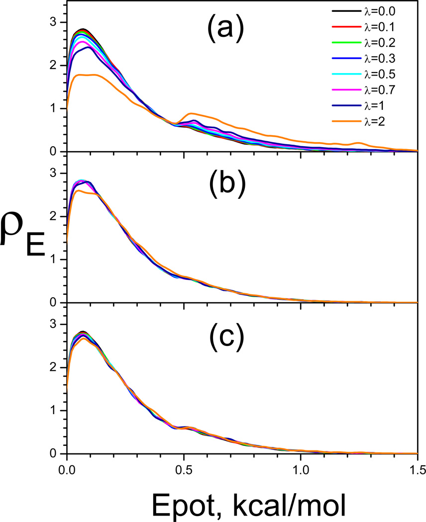
We examine the ensemble distributions from the SGLD and SGLDfp simulations at 80 K with different guiding factors (Fig. 10). The average y-energy of the system at 80 K is 0.107 kcal/mol. The energy barrier height from the average y-energy to the transition energy is 7.24 kT and the energy difference between the two wells is 3.14 kT. Fig. 10 compares the potential energy distributions in the SGLD simulations and the SGLDfp simulations. In SGLD simulations, as can be seen in Fig. 10(a) as λ increases, the distribution decreases in the low energy region and increases in the high energy region. Fig. 10(b) shows the reweighted energy distributions (Wu & Brooks 2011b). Clearly, all curves converge fairly well to the one with λ=0, except when the guiding factor is very large, λ=2, indicating the weighting scheme can convert the SGLD distributions to the canonical. Fig. 10(c) shows the results from the SGLDfp simulations. The densities at different guiding factors converge together, even with λ=2, proving the SGLDfp simulations preserve the energy distribution to a reasonable accuracy.
Fig. 10.
The potential energy distributions of the double well system. (a) SGLD unweighted; (b) SGLD reweighted; (c) SGLDfp. The collision frequency is 10/ps and temperature is 80 K.
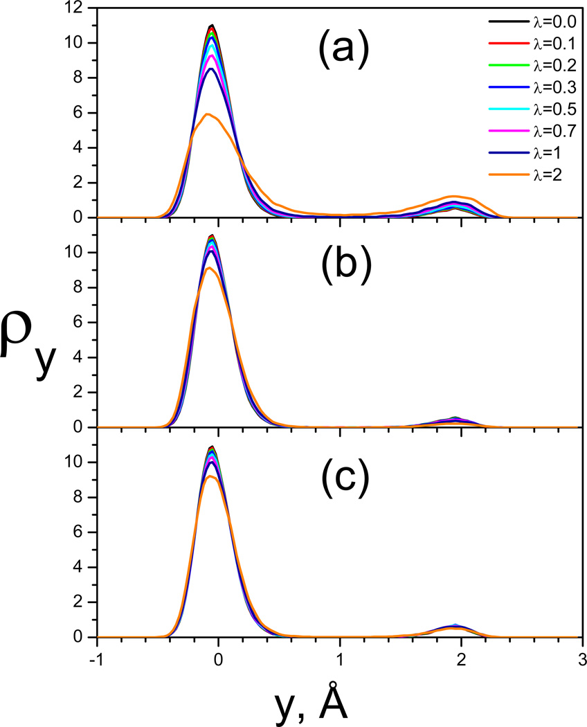
To further demonstrate the preservation in conformational distribution in SGLDfp simulations, we plot the conformational density as a function of the y coordinate in Fig. 11. Fig. 11(a) shows the distributions from SGLD simulations at different guiding factors. There are two peaks with different heights, corresponding to the two skewed double wells. Examining the peak heights at different λ, we can see that as λ increases, the left peak (the higher peak) decreases, while the right peak (the lower peak) grows. Fig. 11(b) shows the reweighted conformational distributions of the SGLD simulations. All distributions converge fairly well to the one with λ=0, except when λ=2, validating the weighting scheme. The SGLDfp results are shown in Fig. 11(c). The densities at different guiding factors almost overlap with each other, except when λ=2, proving the SGLDfp simulation well preserves the conformational distribution. When the guiding factor is too large, here, λ=2, the perturbation of the momentum based guiding force is too large to be described by the reweighting factor or be compensated by the force-based guiding force. These results indicate λ≤1 is the recommended guiding factor range for SGLD reweighting or SGLDfp simulation. This finding is independent of the integration time step of a simulation.
Fig. 11.
The y-coordinate distributions of the double well system. (a) SGLD unweighted; (b) SGLD reweighted; (c) SGLDfp. The collision frequency is 10/ps and temperature is 80 K.
To quantitatively compare the LD result and SGLD, SGLDfp results, we plot the root-mean-square deviations (RMSD) of the SGLD and SGLDfp distributions from the LD result in Fig. 12. The upper panel and lower panel of Fig. 4 show the RMSDs of the energy distributions, δρE, and the RMSDs of the y-distributions, δρy, respectively, for the SGLD simulations before and after reweighting, and for the SGLDfp simulations. The SGLDfp distributions, as well as the reweighted SGLD distributions, show much reduced deviations from the LD distribution than the SGLD distributions. For this system, the SGLDfp distributions and the reweighted SGLD distributions have similar deviations from the LD distributions. The RMSD increase with λ in both the reweighted SGLD result and the SGLDfp result is likely due to statistical noise that increases with the guiding force and the approximation made in separating high and low frequency motion. A more detailed discussion of reweighting accuracy in simulation can be found elsewhere (Shen & Hamelberg 2008). The end result is that both SGLD with reweighting and SGLDfp are sufficiently accurate, when used properly, to both enhance sampling and preserve the ensemble.
Argon fluid
Argon liquid represents a typical homogeneous system. It is a convenient system to examine ensemble average properties. Argon atoms were described by the Lennard-Jones 6–12 potentials with ε=119.8 K and σ=3.405 Å. In this example system, 500 argon atoms were placed in a cubic periodic box (28.53×28.53×28.53 Å3). A time step of 1 fs was used for all simulations. The simulation length was 10 ns for each simulation. The temperature was set to 100 K except otherwise noted. Non-bonded interactions were calculated using the isotropic periodic sum (IPS) method (Brooks et al 2009; Damjanovic et al 2008b; Wu & Brooks 2005). The following rationalized polynomial 3D IPS potentials are used for Lennard-Jones potential calculation:
Lennard-Jones IPS potentials:
| (41) |
| (42) |
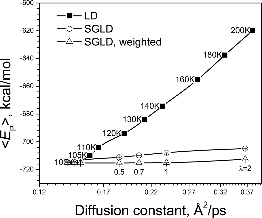
To quantitatively compare the SGLD and high temperature LD simulations, we plot the average potential energies against diffusion constants in Fig. 13. Diffusion constants measure the conformational change in the slowest frequencies and can be a good measurement of conformational search efficiency. The diffusion constants were calculated with a fixed center of mass to avoid any exaggeration due to the enhanced motion of the center of mass. As can be seen from Fig. 13, SGLD increases diffusion constants with much smaller energy deviations than LD simulations at elevated temperatures. This plot tells us that SGLD can speed up conformational searches with little change in conformational distribution, while high temperature LD simulation speeds up conformational search, but searches a conformational space far away from that of the temperature of interest.
Fig. 13.
Average potential energies vs. diffusion constants for the argon liquid in the LD simulations at different temperatures (as labeled) and in the SGLD simulations at different guiding factors (as labeled). The collision frequency is 1/ps. The SGLD simulations were performed at 100 K.
The weighted average potential energies are also plotted against diffusion constants in Fig. 13. For SGLD, the weighted potential energy is very flat against diffusion constant. In other words, through the on-the-fly weighting procedure, SGLD can speed up conformational searches and produce an accurate conformational distribution.
This result also serves as an example that SGLD not only increases the energy barrier crossing rate, but also accelerates the diffusion process. The speed-up in conformational search by SGLD is not only through overcoming energy barriers, but also through enhancing damped low frequency motion.
Alanine dipeptide
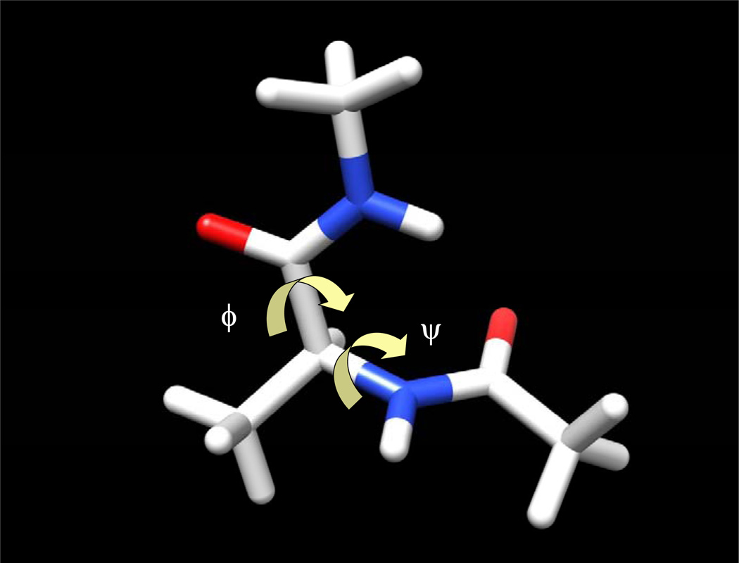
Alanine dipeptide is the simplest molecule that is relevant to proteins. The conformation of this molecule is mainly characterized by two dihedral angles, ϕ: CT-N-Cα-C and ψ: N-Cα-C-NT (Fig. 14). The CHARMM all-atom force field (MacKerell et al 1998) was used to describe the interactions. Here we used a distance-dependent dielectric constant of 4r without cutoffs to represent solvent screening effect to simplify the example.
Fig. 14.
A conformation of an alanine dipeptide. Chemical bonds are shown as sticks. Oxygen and nitrogen atoms are shown as red and blue, respectively. Two backbone dihedral angles, ϕ and ψ, are marked by arrows.
All simulations were performed with a time step of 2 fs and SHAKE algorithm (Ryckaert et al 1977) was employed to fix the bond lengths. Each simulation lasted 200 ns and conformations of every 2 ps were saved for post analysis. The SGLD and SGLDfp simulations were performed with a local averaging time of tL=0.2 ps and a temperature of 300 K. A collision frequency of 10/ps was used for all the simulations.
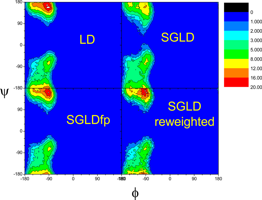
Fig. 15 compares the ϕ–ψ dihedral angle distributions of the alanine dipeptide in LD, SGLD before and after reweighting, and SGLDfp simulations. For this small molecule at the simulation conditions, LD can sample the conformational space fairly well. Comparing the distribution from the LD simulation with that of the SGLD simulation, we can see the one from the SGLD simulation has a lower peak at (−90°, 170°) and a broader baselines near (−50°, 30°), indicating the changing in the ϕ–ψ distribution by the guiding effect in the SGLD simulation. After reweighting, the ϕ–ψ distribution from the SGLD simulation becomes very similar to that of the LD simulation, demonstrating that the SGLD distribution can be converted to the LD distribution through reweighting. Comparing the ϕ–ψ distributions from the SGLDfp simulation and the LD simulation, one can clearly see that they agree with each other fairly well. The root mean square differences from the normalized LD distribution are 1.08, 0.574, and 0.380 for the SGLD distributions before and after reweighting, and the SGLDfp distribution, respectively. These are not fully converged values, and we expect that they would get better with longer simulation time.
Fig. 15.
ϕ-ψ dihedral angle distribution of the alanine dipeptide in the LD, SGLD, and SGLDfp simulations. The collision frequency is γ=10/ps and simulation temperature is 300 K. A guiding factor of λ=1 was used for both the SGLD and SGLDfp simulations.
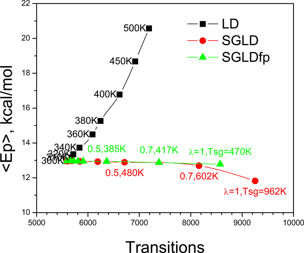
To demonstrate the conformational search ability, we compare the SGLD and SGLDfp simulations with high temperature LD simulations. To quantitatively compare the conformational search ability, we calculated the transition rate for the dihedral angles, (ϕ, ψ) to transfer from one local minimum at (−90°, −70°) to another local minimum at (−90°, 170°). One transfer is counted when (ϕ, ψ) is changing from within 40° of one local minimum to within 40° of the other local minimum.
Fig. 16 shows average potential energy as a function of the transition rate in the high temperature LD simulations as well as in the SGLD and SGLDfp simulations. The average potential energy reflects the conformational distribution to a certain degree. A change in the average energy indicates a change in conformational distribution. As can be seen from Fig. 16, the high temperature simulation increases the transition rate, but also significantly increases the average potential energy. While in the SGLD and SGLDfp simulations, the average potential energy has little change except for the SGLD simulations with λ=1. The transition rate increases significantly with λ in both the SGLD and SGLDfp simulations, even though the SGLDfp simulations have fewer transitions as compared to the SGLD simulations with the same λ. It is also clear from Fig. 16 that the SGLDfp simulation preserves the average energy better. This figure indicates that while the conformational search is accelerated in high temperature simulation, the simulation is searching a conformational space little relevant to that in the folding condition. In other words, the search is enhanced, but the probability of finding the folded conformation may not be enhanced. SGLD or SGLDfp accelerates the conformational search with little change in ensemble distribution, increasing the chance to reach the folded state.
Fig. 16.
Average energies against transition rates in high temperature LD, SGLD, and SGLDfp simulations. The simulation temperatures of the LD simulations, as well as the guiding factors and the self-guiding temperatures of the SGLD and SGLDfp simulations, are labeled beside their data points. The collision frequency is γ=10/ps for all simulations. The simulation temperature is 300 K for the SGLD and SGLDfp simulations.
Folding of a pentamer peptide
Protein folding is a major challenge for conformational search. Due to many degrees of freedom of proteins, the conformational space of a protein is huge and exhaustive conformational search is often impossible. We believe that a reasonable hypothesis of protein folding is that the accessible conformational space for protein is limited and protein can find its folded state quickly by moving through this accessible conformational space. Methods such as high temperature simulations can accelerate conformational search but they also greatly increase the accessible conformational space, which may actually reduce the probability to reach the folded state. Because of the many degrees of freedom, conformational space increases exponentially with the accessibility, while conformational search speed is enhanced with very limited orders of magnitude. An increase in the accessible conformational space not only makes the conformational search problem worse, but also may alter the folding pathway or inhibit folding altogether. The temperature-replica-exchange can enhance sampling while preserving the proper ensemble, but significant difficulties are encountered if the sampled temperatures cross a phase transition at the melting temperature. The SGLD approach avoids the need to generate an ensemble at the many temperatures. The ability to preserve the conformational distribution makes SGLDfp a suitable means to study problems where conformational distribution preservation is critical.
To demonstrate the application of the SGLDfp method in protein folding study, we performed folding simulations for a pentamer peptide (Dyson et al 1988; Wu & Wang 2000), which forms a type II turn according to experimental observation. The sequence of the pentamer peptide is: Tyr-Pro-Gly-Asp-Val. To simplify demonstration, all simulation conditions were the same as that for the alanine dipeptide simulations described above. A temperature of 300 K and a collision frequency of 1/ps were set for all the simulations. The guiding factor was λ=0.5 for the SGLD simulation and was λ=1 for the SGLDfp simulation so both the simulations have similar conformational search ability. All simulations were started from an extended conformation and were 200ns in length.
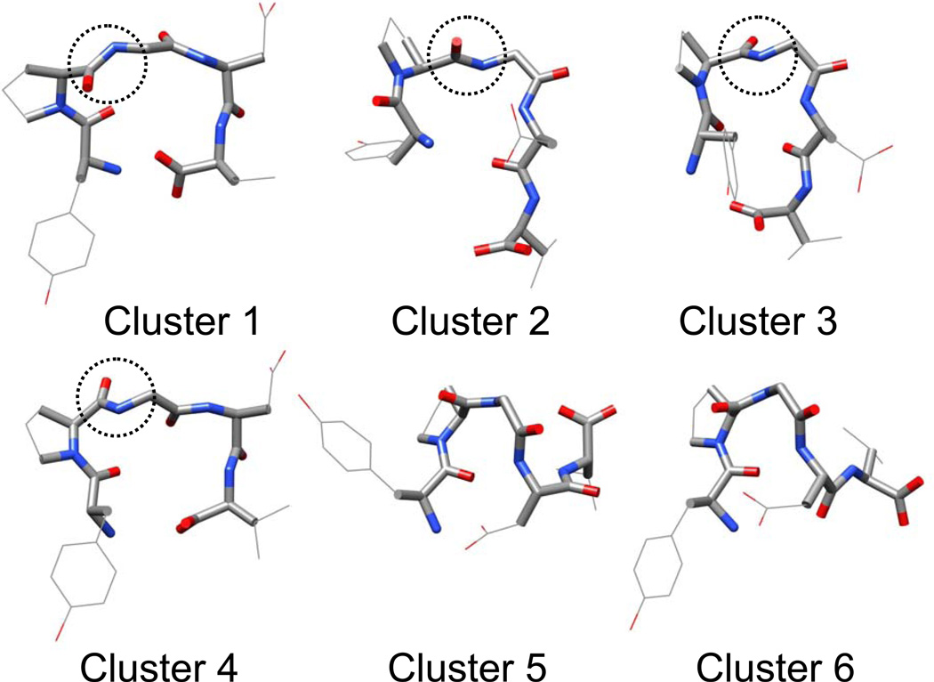
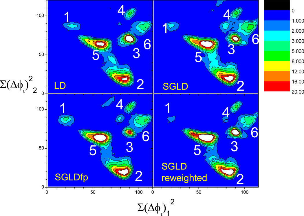
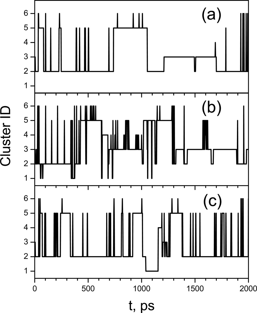
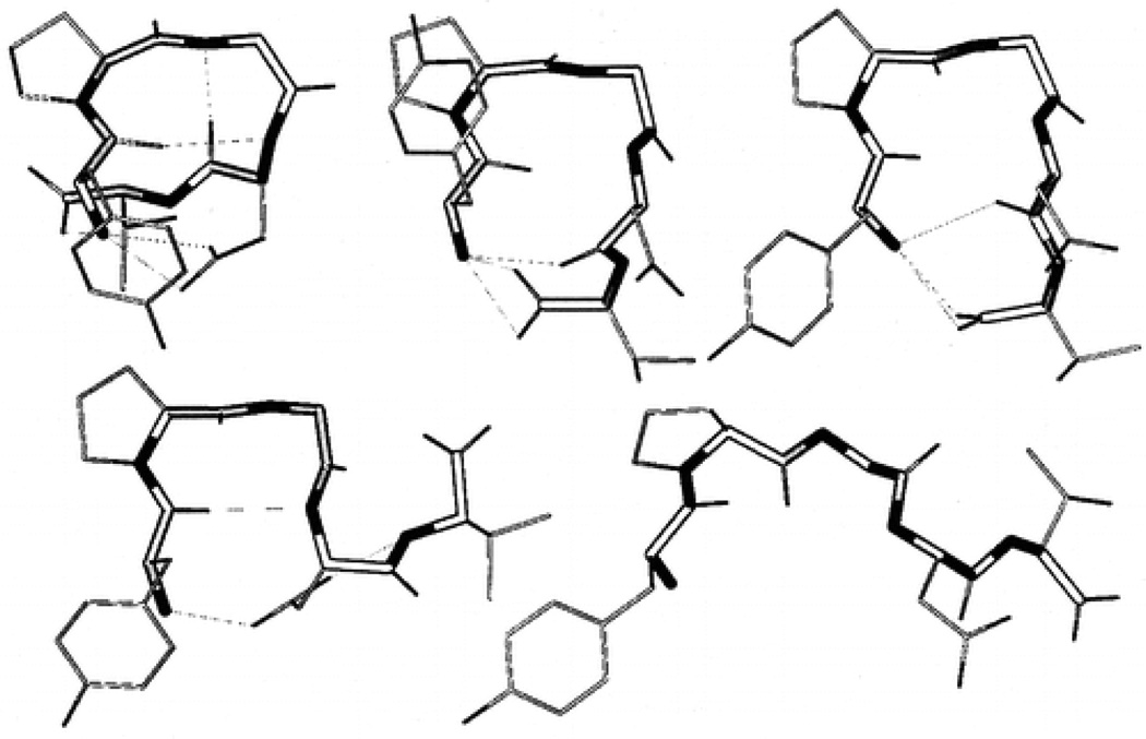
Because a large number of conformations were visited during these simulations, to simplify the description, we clustered the conformations to 6 major clusters using the local maximum clustering method (Wu & Brooks 2004). The distances between conformations are calculated as the sum of the difference square of the backbone dihedral angles. Fig. 17 shows the representative structures of these 6 major clusters. Cluster 1 and 4 have a broad turn involving Pro-Gly-Asp with the proline carbonyl oxygen pointing up and down, respectively. Clusters 2 and 3 have a tight turn involving Pro-Gly with the proline carbonyl oxygen pointing up and down, respectively. Clusters 5 and 6 form a helical coil with a C-terminus pointing up and down, respectively.
Fig. 17.
The representative conformations of the six major clusters of the pentamer peptide. Backbone atoms are shown as thick sticks and sidechain heavy atoms are shown as thin sticks. Hydrogen atoms are not shown for clarity. Atoms are colored grey, blue, red for carbon, nitrogen, and oxygen, respectively.
Fig. 18 compares the conformational distributions obtained from the LD, SGLD, and SGLDfp simulations. The conformational distributions are shown in two-dimensional contour plots with the distances to the center conformations of cluster 1 and 2 as x and y coordinates, respectively. Even though the peptide has only 5 residues, the conformational space is large and the LD simulation of 200 ns may not necessarily properly sample the whole conformational space. All 6 major clusters can be clearly identified in these simulations, even though the SGLD and SGLDfp simulation results have some trace amount of other clusters. The density from the SGLD simulation shows broader peaks than those in LD and SGLDfp results. After reweighting, the SGLD result has peaks as sharp as the other results. The SGLDfp result resembles the LD result fairly well, again demonstrating the SGLDfp method is excellent in preserving the conformational distribution. The RMSDs from the LD result are 1.44, 1.59, and 0.81 for the SGLD results before and after reweighting and the SGLDfp result, respectively. The large RMSD for the reweighted SGLD result is because the reweighting introduces significant noise in the not fully converged distribution plots.
Fig. 18.
Conformational distributions in the LD, SGLD, and SGLDfp simulations. Conformational distances from the center conformations of cluster 1 and 2 are used as x and y coordinates to show the distributions in two dimensions. All simulations are done with γ=1/ps and T=300 K. The guiding factor is λ=0.5 for SGLD and λ=1 for SGLDfp.
Fig. 19 plots the cluster transitions during the first 2 ns simulations. As can be seen, the LD simulation (Fig. 19(a)) did not reach cluster 1 during the first 2 ns simulation and the transitions between clusters are not as frequent as that in the SGLD (Fig. 19(b) and SGLDfp (Fig. 19(c)) simulations. The most frequently transitions were between cluster 2 and cluster 5, which agrees with Fig. 18 in that they are the two major clusters and that they are not separated by a significant barrier. There are also significant transitions between cluster 2 and cluster 3, but not between cluster 2 and cluster 4, agreeing with Fig. 18 that cluster 2 and cluster 4 are separated by clusters 3, 5, and 6. This example demonstrates that SGLDfp is an excellent approach for protein folding study by accelerating conformational search while maintain reasonable conformational distribution.
Fig. 19.
Conformational transitions between the clusters in the first 2000 ps of the LD, SGLD, and SGLDfp simulations. All simulations are done with γ=1/ps and T=300 K. The guiding factor is λ=0.5 for SGLD and λ=1 for SGLDfp.
Applications
Here we review the applications of SGMD and SGLD methods in several scientific areas, including protein folding, modeling of protein structures and complexes, protein conformational rearrangements, water penetration, surface adsorption, crystallization, and phase transitions.
Protein folding
Protein folding is one of the most active areas that utilize molecular simulations. However, studies of protein folding have been hindered by the timescale issues. Protein folding occurs on timescales of microseconds and longer. While several groups have reported MD simulations on a timescale of microseconds and longer, such simulation timescales are still not accessible to a majority of MD simulators. The benchmarking and fine tuning of existing force fields is another problem in the field, and is expected to improve as more and more structures folded through the simulations can be compared with experimental structures. SGMD/SGLD will aid the field of protein folding by easing conformational search limitations.
The earliest application of SGMD in protein folding was in the study of reversible folding of a linear pentamer peptide YPGDV. This peptide was determined by NMR experiments to have a significant population (50%) of a type II turn conformation in aqueous solution (Dyson et al 1988). It was simulated in water with atomic detailed representation for both the peptide and solvent molecules at 300 K using the self-guided molecular dynamics (SGMD) simulation. During a 2 nanosecond (ns) SGMD simulation starting from a fully extended conformation, the peptide folds into a type II turn-like conformation and then undergoes unfolding and refolding several times (Wu & Wang 2000). Simulations with regular MD (Tobias et al 1991; Wu & Wang 2000) failed to reach the experimental observed turn structure in 2 ns. Five major conformational clusters were obtained from the 2 ns SGMD simulation and the most populated conformational cluster is a type II reverse turn-like conformation. The structure of the most populated conformational cluster identified through the SGMD simulations is consistent with the NMR data, and the estimated relative NMR NOE strengths of proton pairs based upon the SGMD trajectory are in good agreement with the experimental data. Fig. 20 shows typical conformational clusters observed during the folding simulation.
Fig. 20.
Five major clusters identified from the trajectory obtained from the 2 ns SGMD simulation (Wu & Wang 2000) (upper row: clusters I, II, and III; lower row: clusters IV and V).
SGMD simulations were further employed to study helix folding in explicit water (Wu & Wang 2001). A 16-residue alanine-based helical peptide (Scholtz et al 1991), Ace-(AAQAA)-Y-NH2, was simulated for 10 ns. The reversible folding (folding, unfolding and refolding) of this peptide in explicit water at 274 K was successfully accomplished. Consistent with experimental results, the helix was found to be the major secondary structural element in aqueous solution, and among different helix forms, the α-helix was the dominant form. Conformational analysis of our simulation results showed that turns and 310-helices play an essential role in the folding of the α-helix. Conventional MD simulations for the same system failed to explore the conformational space in a 10 ns period. An MD simulation started with an extended conformation remained in a random coil structure throughout the 10 ns period as shown in Fig. 21(a), and an MD simulation started with a complete helix remained a complete helix as shown in Fig. 21(b). In the SGMD simulation a variety of conformational states were observed, and their populations are shown in Fig. 22.
Fig. 21.
Snapshots of the peptide conformations obtained in the two 10 ns MD simulations (Wu & Wang 2001): (a) simulation started from a fully extended conformation; (b) simulation started from a complete helix conformation.
Fig. 22.
Major secondary structure clusters observed during the 10 ns SGMD simulation with λ = 0.4 (Wu & Wang 2001). Conformations are clustered on the basis of the number and location of helix segments in the peptide.
β-hairpin folding is a challenge for molecular dynamics simulations due to its long folding time. Using SGMD method, for the first time, β-hairpin folding was directly observed in explicit water simulation (Wu & Brooks 2004; Wu et al 2002). The sequence of the peptide is: Tyr-Gln-Asn-Pro-Asp-Gly-Ser-Gln-Ala. Strong NMR NOE evidence indicates that this peptide folds into a β-hairpin structure in aqueous solution (Blanco et al 1993). Reversible folding process of this β-hairpin was simulated with the SGMD method, and details of the folding process were analyzed. Fig. 23(a) shows a typical β-hairpin structure observed in the simulations. This structure was first reached in about 20 ns. Fig. 23(b) shows the excellent agreement between the experimental NOEs and the average distances of the corresponding atom pairs.
Fig. 23.
Reversible b-hairpin folding simulation with SGMD (Wu & Brooks 2004; Wu et al 2002). (a) A typical folded structure of the peptide obtained in the simulation (at 21,000 ps). For clarity, side chain hydrogens are not shown. The backbone atoms are shown as thick sticks and side chain atoms as thin sticks. Interstrand hydrogen bonds are marked by dashed lines. Atoms are colored red for oxygen, blue for nitrogen, white for hydrogen, and green for the rest. (b) NMR NOEs observed in the peptide aqueous solution2 (arrow bars between residues) and the average hydrogen pair distances (numbers in Å above NOE bars) in the β-hairpin structure obtained in our simulation. α, N, sc, and b represent the hydrogen atoms on α-carbon, amide nitrogen, side chain (β-carbon in our calculation), and backbone (amide nitrogen in our calculation). The thickness of the NOE bars represents the strength of the NOEs reported. Generally, NOEs are strong for hydrogen pair distances within 3 Å, medium between 3 and 4 Å, and week between 4 and 5 Å.
Recently Lee and Olson combined SGLD with temperature based replica-exchange to perform protein folding simulation (Lee & Olson 2010). They tested the performance and accuracy of the MDReX, LD-ReX and SGLD-ReX simulations for the prediction of thermodynamic folding observables of the Trp-cage mini-protein. The PARAM22+CMAP force field was used together with the generalized Born molecular volume implicit solvent model. They found that the SGLD-ReX folds up the protein several times somewhat faster than the two conventional ReX approaches, in contrast to the 65-fold speedup of helix formation reported in the original SGLD paper (Wu & Brooks 2003). The likely explanation is that ReX already provides sufficient sampling enhancement for MD and LD to overcome the unfolded/folded transition barrier to fold up the trp-cage. Their result suggests that SGLD-ReX improves sampling convergence by reducing topological folding barriers between energetically similar near-native states. Also, they found that SGLD-ReX predicted the melting temperatures, heat capacity curves, and folding free energies that are closer in agreement to the experimental observations. Fig. 24 shows the energy and RMSD distribution in MD-Rex, LD-Rex, and SGLD-Rex. All three methods sample the nearest-to-native basin (1 Å) at their respective transition temperatures, with SGLD-ReX having the most density there. Since the nearest-to-native basin does not appear to be the lowest in free energy, this could be due to the fact that SGLD-ReX performs the most excursions among basins in a given simulation time. Another positive feature of SGLD-ReX shown in Fig. 24(g)–(i) is how similar the PMFs are among the different starting conformations and data collection times. This suggests that, of the three methods, SGLD-ReX is the most self-consistent and arguably the most converged, at least in the conformational space of compact folds. The 150–200 ns data windows of MD-ReX and LD-ReX do have qualitative agreement with SGLD-ReX, suggesting that longer equilibration times could bring these three methods into better agreement.
Fig 24.
Combined SGLD with replica-exchange in protein folding simulation (Lee & Olson 2010). Free-energy landscapes at respective melting temperatures (ΔGfold = 0) of individual simulations method/starting structure/simulation data〉 in the coordinates of potential energy, U, and Cα rmsd to native: (a) MD-ReX/trans/50–100 ns (T = 351.3 K), (b) MD-ReX/native/50–100 ns (T = 354.6 K), (c) MD-ReX/native/150–200 ns (T = 348.2 K), (d) LD-ReX/trans/50–100 ns (T = 290.1 K), (e) LD-ReX/native/50–100 ns (T = 335.1 K), (f) LD-ReX/native/150–200 ns (T = 353.9 K), (g) SGLD-81 ReX/trans/50–100 ns (T = 311.2 K), (h) SGLD-ReX/native/50–100 ns (T = 331.5 K), and (i) SGLDReX/native/150–200 ns (T = 306.4 K).
Lee and Change characterized the denatured state of the human prion (huPrP) 121–230 through SGLD simulations (Lee & Chang 2010). Misfolding and aggregation of the prion protein (PrP) are responsible for the development of fatal transmissible neurodegenerative diseases. To gain insight into possible aggregation-prone denatured states, multiple SGLD simulations started from the extended conformation of the huPrP 121–230 were performed. The simulations were performed with an implicit solvent and were 50 ns long. The structural analysis indicated that the most populated denatured state of huPrP is partially folded with helical content. Experimental observation indicated that PrP fibril is rich in β-sheet structure. Lack of β-structure suggests that β-sheets in amyloid fibrils may be formed from inter-molecular interactions rather than intra-molecular forces. Fig. 25 shows the partially unfolded structure of huPrP 121–230.
Fig. 25.
Characterization of prion denatured state with SGLD simulations (Lee & Chang 2010). (A) The NMR structure of huPrP121–231 (PDB 1hjn [19]), (B) fully unfolded huPrP 121–230 at 600 K with the disulfide-bond shown in red, and (C) the simulated denatured structure of huPrP from the most populated cluster. The helical regions I, II and III defined based on the native structure are colored in red, blue and magentas, respectively.
Wen and coworkers have studied protein folding with Poisson–Boltzmann molecular dynamics with self-guiding forces (SG-PBMD)(Wen et al 2004). They investigated the sampling efficiency with SGPBMD in molecular dynamics with the PB implicit solvent when self-guiding forces are added. They found an impressive efficiency as measured by fluctuations of potential energy, radius of gyration, backbone RMSD, and by the number of unique clusters, and distribution of low RMSD structures over time compared with a high-temperature dynamics simulation. They performed ab initio folding simulations of BBA1 and villin headpiece, and discussed folding pathways for the two small proteins. They found topological agreement between the folded state observed in their simulation and the theoretical native states (Fig. 26). The denatured state of the BBA1 miniprotein was discussed in more detail in a subsequent publication (Wen & Luo 2004).
Fig. 26.
Poisson-Boltzmann molecular dynamics simulation with the self-guiding force (Wen et al 2004; Wen & Luo 2004). Superposition of theoretical native states (gray) and native-like structures found in folding simulations (black): (a) BBA1; (b) villin headpiece.
Molecular modeling and docking
Characterization of the solution structure of peptides has been the goal of many simulation studies. Yang et al. used SGMD to study solution conformations of wild-type and mutated Bak BH3 peptides via dynamical conformational sampling (Yang et al 2004). The BH3 domain of the Bcl-2 family of proteins plays a critical role in the regulation of apoptosis. Their SGMD simulations showed that the Bak peptide exhibits a partially formed helical structure with a fairly stable 6-residue helical segment at the N terminus and a less stable approximately 4-residue helical segment at the C terminus. Additional SGMD simulations of two mutated Bak peptides, found that the R5G mutation greatly affects the solution conformations of the peptide, and the overall helix ratio decreases by a factor of 2 as compared to the wild-type Bak peptide, but that the R5A mutation does not affect significantly the peptide solution conformations observed in the wild type. To quantitatively examine the effects of mutations on each residue, they calculated the helical propensity for each residue from the 10-ns simulations for these three peptides (Fig. 27). Analysis of representative conformations of the R5A mutant suggested that the relatively stable helical segment close to the N terminus may greatly facilitate its binding to Bcl-xL.
Fig. 27.
Bak BH3 simulation results with SGMD (Yang et al 2004). Effects of mutation on the helical propensity from the 10-ns wild type and R5G and R5A sampling simulations.
Chandrasekaran et al utilized SGMD in modeling of a protein complex between the protein Z-dependent protease inhibitor (ZPI) and the factor Xa (FXa), a serine protease that plays a key role in the blood coagulation cascade (Chandrasekaran et al 2009). The Michaelis complex of human ZPI/FXa was built using homology modeling, protein–protein docking and molecular dynamics simulation methods. The ZPI/FXa complex built through the docking method was subjected to SGMD simulation, to enhance conformational sampling efficiency. The aim was to examine whether the conformation of ZPI/FXa obtained through docking moved towards the conformation obtained through homology modeling or if it explored a different conformational path. The motivation behind using accelerated conformational sampling was to obtain a qualitative idea, in a reasonable timescale, regarding the direction of movement of ZPI in the ZPI/FXa complex obtained through the docking method. Fig. 28 shows the complex model they obtained.
Fig 28.
Solvent equilibrated models for protein z-dependent protease inhibitor and its initial reactive complex with coagulation factor Xa (Chandrasekaran et al 2009).
Understanding the fundamental principles that govern the binding of a guest molecule to its host and accurate prediction of the binding mode of the guest/host complex are important goals in guest–host chemistry and have implications in structure-based drug design. Varady et al performed a computational investigation of benzyl alcohol (the guest) binding to β-cyclodextrin (the host) in the presence of explicit water molecules (Fig. 29) using both SGMD and conventional MD simulations (Varady et al 2002). In their SGMD simulations, competitive and reversible binding of the guest molecules to the host is observed. Analysis of the simulation trajectories (Fig. 30) showed that one major complexed conformational cluster is in good agreement with the complex structure determined using X-ray diffraction method. In addition, several other major binding modes were also identified in aqueous solution. Investigation of the binding forces showed that the burial of the phenyl group in the cavity of β-cyclodextrin, but not the hydrogen bonding interaction between the guest and the host, is the major change for binding, suggesting that that hydrophobic interaction may be responsible for the formation of the complex. To verify the predictions made by the SGMD method, two 12.5 ns conventional MD simulations with the same initial setup and same conditions as for the two SGMD simulation runs were performed. Additionally, a 10 ns long conventional MD simulation starting from the crystal structure of the complex was performed. The MD simulations predicted major solution binding modes similar to those identified through the SGMD simulations, including the conformational cluster that is essentially the same as that found in the X-ray structure. The studies showed that the SGMD method is an efficient way to study competitive and reversible binding of guest molecules to their hosts in aqueous solution. This study result indicates that SGMD may also be useful to study the binding of drug molecules to their marcomolecular targets.
Fig. 29.
Guest-host binding simulation with SGMD (Varady et al 2002). Starting Conformations for SGMD (SGMD #1 and #2) and Corresponding MD Simulations (MD #3 and #4). For clarity, only heavy atoms are shown. The six benzyl alcohol molecules are either all around the “rim” of the host (top) or four around the rim, one “below” and one “above” β-cyclodextrin (bottom).
Fig. 30.
Distance between the centers of the mass of guest and host molecules during MD and SGMD simulations (Varady et al 2002). For clarity, we plotted only the distances for guest molecules, which become tightly bound (within 3 Å) to the host molecule for longer than 30 ps during simulations.
Lung et al used SGMD to study conformations of small peptide (called G1) that binds to the Grb2-SH2 domain but not the src SH2 domain (Lung et al 2001). G1 is a candidate to be an inhibitor for the function of the Grb2-SH2 domain which binds to specific tyrosine-phosphorylated motifs on activated GF receptors. Overexpression of these receptors, or constitutive activation of this pathway, is highly relevant to a number of diseases, including breast cancer. Thus, blocking Grb2-SH2 function provides a promising therapeutic target for the development of new antitumor agents. Conformations of the G1 peptide in explicit solvent were generated with the SGMD simulations. For the SGMD simulations, the local averaging time t1 was set at 2 ps and the guiding factor was set at 0.5. The four major conformational clusters of G1 identifed from an SGMD simulations are shown in Fig. 31. Molecular modeling studies suggest that the G1 peptide can adopt low-energy solution conformations, which allow its Tyr3 and Asn5 to mimic the corresponding pTyr and Asn residues in the natural phosphopeptide ligand. Moreover, its Glu1 residue can interact with the positively charged binding site in Grb2-SH2, thus partially compensating for the absence of a phosphate group in G1 for its strong interaction with Grb2-SH2.
Fig. 31.
Four major conformational clusters of G1 identified from an SGMD simulation in explicit water (Lung et al 2001). These clusters were identified using all 500 conformations recorded during the 500 ps SGMD simulation. The conformations in conformational cluster (A) were similar to the starting conformation, whereas the conformations in the other three clusters were substantially different from the starting conformation, and exhibited circular open-chain backbone conformations lacking evidence of intramolecular interactions.
Due to the enhanced conformational search ability of SGMD/SGLD, this method is often used as an efficient way to explore conformational space. Shao et al (Shao et al 2007) used MD and SGMD as a tool to generate conformational library to test different clustering algorithms. In case of a 10-mer polyadenine single strand of DNA standard 5 ns long MD simulations yielded conformations that were fully stacked and helical on a 5 ns time scale. SGMD was used to generate single strand structures more representative of the true ensemble and to generate a set of diverse conformations for clustering. SGMD parameters that were utilized were significantly greater than those routinely applied. When used in this manner, the SGMD rapidly moves the DNA and effectively samples a very wide range of “unfolded” conformations in short (1 ns) runs. Configurations generated with SGMD were then used as starting structures for a standard MD run. The structures generated with MD where further used for clustering.
Protein conformational transitions
Protein conformational transition plays a central role in key cellular processes such as signal transduction. Due to the large size of protein systems and long time scale of transition events, describing such events has been a challenge for simulation studies. The SGLD method has been used successfully to provide qualitative insights into the mechanisms and types of conformational relaxation that occur upon ligand binding.
Damjanovic et al applied SGLD to study protein conformational reorganization triggered by charging of internal ionizable residue in three variants of protein staphylococcal nuclease (SNase)(Damjanovic et al 2008b). SGLD simulations with five different sets of guiding parameters (including λ=0, i.e., no guiding) were performed and compared to each other, as well as to the structural information available through CD, steady state Trp fluorescence and NMR spectroscopy. Simulations of the wild type protein, which does not contain internal ionizable residues and does not undergo conformational transitions served to calibrate and benchmark the simulations. Comparison of the amount of backbone relaxation in the wild type protein as measured through the average secondary structure content showed only small amounts of secondary structure loss, exclusively localized to the termini of β-strands and α-helices. The observations were consistent between SGLD and LD simulations, with the SGLD simulations with λ=1 exhibiting slightly smoother transitions at helical termini. In contrast to the wild type protein, the three variants that contain internal ionizable residues exhibit experimental evidence of structural relaxation triggered by charging of internal groups. Fig. 32 shows the secondary structure changes during the SGLD simulations. The structural trends observed in the simulations are in general agreement with experimental observations. The I92D variant, which unfolds globally upon ionization of Asp-92, in simulations often exhibits extensive hydration of the protein core, and sometimes also significant perturbations of the β-barrel. In the crystal structure of the V66R variant the β1 strand from the β-barrel is domain swapped; in the simulations the β1 strand is sometimes partially released. The V66 K variant, which in solutions shows reorganization of six residues at the C-terminus of helix α1 and perturbations in the β-barrel structure, exhibits fraying of three residues of helix α1 in one simulation, and perturbations and partial unfolding of three β strands in a few other simulations. Overall, the use of SGLD simulations was shown to facilitate observation of conformational transitions in proteins where such conformational relaxation is believed to exist.
Fig 32.
SNase conformational reorganization from SGLD simulations (Damjanovic et al 2008b). The residues undergoing change in the secondary structure are shown in red. The substituted ionizable groups are shown in stick representation.
In another study of variants of the V66E variant of SNase (Damjanovic et al 2008a), SGLD was benchmarked against LD in its ability to reproduce hydration state and rotameric substates of internal Glu-66 side chain, when the side chain is in a neutral state (Fig. 33). Because of the intricate coupling between the hydration state and rotameric states of this internal side chain, the correct sampling of side chain conformations may require very long simulation times. Alternatively, multiple simulations started with different initial velocities can achive more effective sampling of side chain conformations. In this study, populations of two side chain conformations were studied based on 40 short LD and SGLD simulations. The results of simulations with LD and SGLD methods yield side chain and water populations that agree up to 8%. In contrast, the results of simulations started with and without the crystallographic water molecules differed by as much as 20%. We note however, that the simulations were not fully converged, and that with additional simulation time the simulations with different initial hydration states should have converged to the same value. Similarly, the differences in populations observed in simulations with the SGLD and LD could likely be attributed to the difference in sampling efficiency of the two methods during the same simulation time. Surprisingly, when performance of SGLD in sampling of conformational transitions was benchmarked it was found that the number of hops between the two conformations of the side chain was only slightly larger in SGLD than in LD (228 vs 191). We believe that this is because the conformational transitions in this case were heavily influenced by the fluctuations in the hydration state of the side chain. The hydration state of the side chain was dependent on the penetration and exiting of water molecules from the protein interior and the guiding parameters used in the study most likely do not enhance such motions.
Fig. 33.
Crystal structure of the V66E variant of SNase (Damjanovic et al 2008a). (right) Snapshots from MD simulations representative of the straight (left) and the twisted (right) conformation of the Glu-66 side chain.
Conformational transitions induced by dephosphorylation in the NtrC protein was studied through multiple SGLD simulations (Damjanovic et al 2009). SGLD simulations provided a way to examine structural and dynamical properties of the receiver domain of nitrogen regulatory protein C (NtrCr) and study pathways of conformational transitions induced by dephosphorylation. NtrC is a signaling protein regulated by phosphorylation of an Asp-54 residue in NtrCr. It is believed that that the protein undergoes conformational transitions between inactive and active forms on a μ second timescale. Phosphorylation of NtrCr stabilizes the active form of the protein. The major structural difference between the two forms is in the orientation of the regulatory helix α4. SGLD and MD simulations of the phosphorylated active form structure suggest a mostly stable but broad structural ensemble of this protein. The finite difference Poisson–Boltzmann calculations of the pKa values of the active site residues suggest an increase in the pKa of His-84 on phosphorylation of Asp-54. In SGLD simulations of the phosphorylated active form with charged His-84, the average position of the regulatory helix α4 is found closer to the starting structure than in simulations with the neutral His-84. To model the transition pathway, the phosphate group was removed from the simulations. After 7 ns of simulations, the regulatory helix α4 was found approximately halfway between positions in the NMR structures of the active and inactive forms. Even though the simulations were too short to observe the full range of conformational transitions between the active and inactive forms of the protein, the study illustrates the potential utility of the SGLD method in providing the atomic level details about the pathways of conformational transitions and role of particular residues in conformational transitions induced by ligand binding/unbinding.
SGLD was recently used to study conformational changes in a membrane transporter protein lactose permease (LacY)(Pendse et al 2010). LacY undergoes a conformational change from a state that is open to the cytoplasm to the state that is open to the periplasm in response to sugar binding and protonation of Glu-269 residue (Fig. 35). SGLD simulations were used to enhance conformational sampling in simulations of LacY with implicit description of the membrane. SGLD simulations were followed by MD simulations with an explicit description of a fully hydrated bilayer. Control simulations without the sugar bound and without the protonated Glu-269 were performed to verify that in this case there are no conformational changes in the periplasmic half. Indeed, only simulations with the sugar bound and with the protonated Glu-269 resulted in conformational changes in the periplasmic half. In those simulations the pore radius of the lumen increased by 3.5 Å on the periplasmic side, while the pore radius decreases by 2.5 Å on the cytoplasmic side. SGLD simulations were found to enhance observations of structural changes. The periplasmic open conformations were found to agree with experimental data. The comparison with the experiments suggest a possible incomplete closure of the cytoplasmic side, however, large enough to prevent the sugar from being transported to the cytoplasm (Pendse et al 2010).
Fig. 35.
SGLD study of conformational changes in a membrane transporter protein lactose permease (LacY)(Pendse et al 2010). Proton translocation to Glu269 and sugar binding trigger LacY conformational change from the inward-facing to the outward-facing state
Surface adsorption
SGMD simulations were used to study adsorption of the ionic complementary peptide EAK16-II on the hydrophobic HOPG surface (Fig. 36)(Sheng et al 2010a; 2010b). Protein adsorption plays an important role in bioactive implant devices and drug delivery materials design. Ionic complementary peptides are novel nanobiomaterials with many biomedical applications, and understanding of the fundamentals of peptide adsorption on the surface is important for peptide applications in biotechnology and nanotechnology. The studies examine the roles of the hydrophobic interaction, electrostatic interactions and hydrogen bonding interactions on the adsorption of the peptide molecules under neutral, acidic and basic conditions. Fig. 37 shows the snapshots of the peptide EAK16-II on the HOPG surface.
Fig. 36.
Molecular dynamics simulations of the ionic complementary peptide EAK16-II on the hydrophobic HOPG surface (Sheng et al 2010a; 2010b). The adsorption and initial assembly process of EAK16-II on the surface were revealed. Hydrophobic alanine residues are found to be energetically favorable when in contact with the HOPG surface. It is the hydrophobic interaction that drives the adsorption of the first peptide molecule.
Fig. 37.
Snapshots of the peptide EAK16-II on the HOPG surface (Sheng et al 2010a; 2010b). The carbon atoms consisting of the HOPG surface are colored in cyan, water molecules are colored in red. The two peptide molecules are displayed with vdW spheres, and the three residues alanine, glutamic acid, and lysine are colored in grey, red, and blue, respectively.
Crystallization and Phase Transitions
Argon crystallization was studied with SGMD (Wu & Wang 1999). A system of 500 argon atoms was used in the simulations, as shown in Fig. 38. The starting structure was created by melting a fcc crystal at 120 K, cooling down, and equilibrating at 60 K. The equilibrated argon liquid film was simulated using the conventional MD method and the SGMD method at tL = 0.2 ps and λ= 0.02, 0.05, and 0.1. In the conventional MD simulation, it took 65 ns before crystallization occurred. In the SGMD simulations, the crystallization occurred at 63, 2, and 0.5 ns with λ= 0.02, 0.05, and 0.1, respectively. Figure 39 shows the potential energy changes during these simulations. Phase transitions are evident by the sharp decline in potential energy.
Fig. 38.
Crystallization of argon liquid observed in SGMD simulations (Wu & Wang 1999). Snapshots of the argon film system at T* = 0.501(60 K). (a) Initial liquid structure, (b) crystallized structure. A tetragonal periodic boundary condition with sides a = b = 28.53 Å along x- and y-axes and c = 57.06 Å along z-axis is applied to the system.
Fig. 39.
The potential energies of the super-cooled argon film system (T* = 0.501) during the crystallization simulations (Wu & Wang 1999). Simulations were T* = 0.501 and with tl = 0.2 ps and different values. The solid line represents the results from a conventional MD simulation. The dashed line, dotted line, and centered lines represent the results in the SGMD simulations with tl = 0.2 ps and = 0.02, 0.05, and 0.1, respectively.
Sinoda and Mikami extended the SGMD method to the isotermal-isobaric ensemble and applied it to study crystallization of argon fluid in a supercooled state (Shinoda & Mikami 2001). They found that the pressure-induced and temperature-induced crystallization was considerably accelerated with the use of suitable parameter set in the SGMD method, as long as the system is not in a glass state.
Production of amorphous silicon has been simulated with SGMD (Choudhary & Clancy 2002; 2005a; 2005b). Choudhary and Clancy used the SGMD method to study evolution of a quenched sample of liquid silicon. The validity of the results using SGMD was provided by comparison to a conventional molecular dynamics MD algorithm simulated under constant temperature conditions for more than 100 ns. They found that it was important to perform a sensitivity analysis of the effect of the SGMD parameters before applying the self-guided MD scheme. They demonstrated that using a suitable set of parameters in the SGMD method improved the structural evolution as compared to a conventional MD scheme, even in the glass state. They concluded that SGMD provides an important tool for observing the evolution of slowly changing processes.
SGMD was used to study phase transformation of Cu precipitate in Fe-Cu alloy (Tsuru et al 2010),(Abe & Jitsukawa 2009). It was shown that the SGMD method can accelerate calculating the bcc to 9R structure transformation of a small precipitate, enabling the transformation without introducing any excess vacancies. Fig. 40 compares the size of the Cu precipitate at which the phase transformation occurs in conventional MD, simulated annealing MD (SAMD), and SGMD. In conventional MD and in SAMD, phase transformation occurred when the precipitate was larger than 5.0 nm and 6.0 nm respectively. However, in the SGMD simulation, the size of the Cu precipitate needed to change the coordination number was 4.0 nm, which is in good agreement with the lower bound of what was experimentally observed.
Fig. 40.
Comparison of phase transition process in different simulations (Abe & Jitsukawa 2009). Coordination number with respect to the size of Cu precipitates in conventional MD, simulated-annealing MD (SAMD), and SGMD (λ=0.1, tL=0.2ps).
Summary
Since the development of the SGMD (Wu & Wang 1998; 1999) and SGLD (Wu & Brooks 2003) methods, they have been employed to study many slow processes and events. A theoretical understanding of the methods was achieved only after recent progress in quantitative description of SGLD ensembles (Wu & Brooks 2011a; 2011b). The low frequency motion defined by the local averaging time, tL, determines the efficiency of conformational search. Energy barriers and diffusion limits are among the causes of slow low frequency motion. The enhancement in conformational search efficiency in SGLD simulations is achieved through transferring kinetic energy from high frequency degrees of freedom to low frequency degrees of freedom so that the low frequency motion is accelerated while the high frequency motion is suppressed. Once a barrier is crossed, the excess energy is returned to the high frequency degrees of freedom. We refer to this effect as “energy borrowing”, and it can occur with minimal effect on the overall conformational distribution.
The guiding force can have various compositions which will lead to various forms of SGLD simulation method (Table I) depending on how the guiding force is calculated. When the friction constant is reduced to zero, an LD simulation is reduced to an MD simulation and the SGLD simulation method is transferred to the SGMD simulation method. Depending on how the guiding force is calculated, SGLD can be transformed to SGLDf, SGLDfp. And when the friction constants reduces to zero, SGLD is transformed to SGMDf, SGMDp, or SGMDfp. When only non-bonded forces are used for the guiding force calculation, it is transformed to the original SGMD simulation method.
The partition function of an SGLD ensemble can be expressed with the low frequency and high frequency properties. From the SGLD partition function, we can convert SGLD conformational distribution to a canonical conformational distribution, and canonical ensemble averages can be calculated in SGLD simulations through reweighting either on-the-fly or during post processing. It should be noted that the reweighting approach becomes intractable for large systems where the range of the reweighting factors can be large. In this case the convergence is poor because the reweighting approach is not size extensive.
The SGLDfp method incorporates both the local average momentum and local average force in such a way that a canonical ensemble conformational distribution is directly sampled. Therefore, the SGLDfp approach can directly sample the canonical conformational space while accelerating conformational search, and can be used in conjunction with many other techniques, such as umbrella sampling or free energy perturbation, to improve convergence. The SGLDfp approach is seen to be size extensive. Doubling the size of the system does not seem to impact the quality of the distribution.
The enhanced conformational search ability can be measured by the self-guiding temperature, Tsg, which is calculated with the low frequency temperature and high frequency temperature of an SGLD simulation. An SGLD simulation with a self-guiding temperature of Tsg will have a conformational searching ability comparable to a high temperature simulation at T = Tsg. In a typical SGLD simulation, one can expect Tsg = 2T. In other words, a typical SGLD simulation has an enhanced conformational searching ability comparable to a high temperature simulation with its temperature doubled.
The performance of an SGLD simulation can be turned with three parameters, the guiding factor, λ, the local averaging time, tL, and the collision frequency, γ. λ determines the strength of the guiding effect and is recommended to take values between 0 and 1. When λ=0, an SGLD simulation reduces to an LD simulation and if γ=0, an SGLD simulation reduces to an MD simulation. tL determines which low frequency motion to be enhances and which high frequency motion to be suppressed. tL =0.2 ps is default for an SGLD simulation which has been used for secondary structure folding simulations. For lower frequency motions like protein domain motion, larger tL, say 1 ps, would be more suitable. This value range for various types of molecular motion will be the topic of future studies. γ is related to the diffusion in a simulation system. Also, γ is a factor in the guiding force calculation. Therefore, increasing γ will slow down thermal diffusion and increase the guiding effect. Considering these competing two effects, there is an optimal γ value that maximizes the conformational search ability.
Temperature based replica-exchange method has been widely used in conformational search and sampling. However, for large systems, many replicas with small temperature difference are needed to have reasonable transition rate. The quantitative understanding of the SGLD partition function make it possible to perform guiding factor based replica-exchange simulation at a constant temperature.
The SGLDfp is unique in that it greatly enhances sampling while directly preserving the canonical ensemble. It is an ideal approach to problems where ensemble distribution preservation is critical, such as protein folding and pathway studies, or when computing free energies.
SGLD and SGLDfp can also be used in conjunction with many other sampling techniques that currently rely on MD or LD to sample conformational space. As an efficient and accurate simulation approach, we believe SGLD will play an important role in molecular simulation studies of processes such as protein folding, structure prediction, conformational arrangements, free energy calculations, binding mode prediction, as well as protein function studies.
Figure 34.
SGLD simulation of Conformational transitions induced by dephosphorylation in the NtrC protein (Damjanovic et al 2009). A) NMR structure of the inactive form of NtrCr. The key helix 4 is shown in black. B) NMR structure of the active form of NtrCr. C) Conformations of the key helix, 4: dark gray and white are the NMR structures of the phosphorylated and dephosphorylated forms, respectively. In blue is the average structure from the SGLD simulations of the phosphorylated protein. In green and red are the average structures from the SGLD simulations of the dephosphorylated protein with His-84 neutral and protonated, respectively.
Acknowledgment
This research was supported by the Intramural Research Program of the NIH, NHLBI. A.D. was partially supported by NIH Grant RO1 GM073838 to Bertrand Garcia-Moreno at Johns Hopkins University.
Contributor Information
Xiongwu Wu, Email: wuxw@nhlbi.nih.gov.
Ana Damjanovic, Email: adamjan1@jhu.edu.
Bernard R. Brooks, Email: brb@nih.gov.
References
- Abe Y, Jitsukawa S. Phase transformation of Cu precipitate in Fe-Cu alloy studied using self-guided molecular dynamics. Philosophical Magazine Letters. 2009;89:535–543. [Google Scholar]
- Adcock SA, McCammon JA. Molecular dynamics: Survey of methods for simulating the activity of proteins. Chemical Reviews. 2006;106:1589–1615. doi: 10.1021/cr040426m. [DOI] [PMC free article] [PubMed] [Google Scholar]
- Allen MP, Tildesley DJ. Computer Simulations of Liquids. Oxford: Clarendon Press; 1987. [Google Scholar]
- Andricioaei I, Dinner AR, Karplus M. Self-guided enhanced sampling methods for thermodynamic averages. J. Chem. Phys. 2003;118:1074–1084. [Google Scholar]
- Beckers ML, Buydens LM, Pikkemaat JA, Altona C. Application of a genetic algorithm in the conformational analysis of methylene-acetal-linked thymine dimers in DNA: comparison with distance geometry calculations. J Biomol NMR. 1997;9:25–34. doi: 10.1023/a:1018667416967. [DOI] [PubMed] [Google Scholar]
- Blanco FJ, Jim,nez MA, Herranz J, Rico M, Santoro J, Nieto JL. NMR Evidence of a Short Linear Peptide That Folds into a á-Hairpin in Aqueous Solution. J. Am. Chem. Soc. 1993;115:5887–5888. [Google Scholar]
- Brooks BR, Brooks Iii CL, Mackerell AD, Jr, Nilsson L, Petrella RJ, et al. CHARMM: The biomolecular simulation program. Journal of Computational Chemistry. 2009;30:1545–1614. doi: 10.1002/jcc.21287. [DOI] [PMC free article] [PubMed] [Google Scholar]
- Brooks BR, Bruccoleri RE, Olafson BD, States DJ, Swaminathan S, et al. CHARMM: A program for macromolecular energy, minimization, and dynamics calculations. J. Comput. Chem. 1983;4:187–217. [Google Scholar]
- Brower RC, Vasmatzis G, Silverman M, Delisi C. Exhaustive conformational search and simulated annealing for models of lattice peptides. Biopolymers. 1993;33:329–334. doi: 10.1002/bip.360330302. [DOI] [PubMed] [Google Scholar]
- Brown WM, Faulon JL, Sale K. A deterministic algorithm for constrained enumeration of transmembrane protein folds. Comput Biol Chem. 2005;29:143–150. doi: 10.1016/j.compbiolchem.2005.03.001. [DOI] [PubMed] [Google Scholar]
- Budin N, Ahmed S, Majeux N, Caflisch A. An evolutionary approach for structure-based design of natural and non-natural peptidic ligands. Comb Chem High Throughput Screen. 2001;4:661–673. doi: 10.2174/1386207013330652. [DOI] [PubMed] [Google Scholar]
- Bussi G, Gervasio FL, Laio A, Parrinello M. Free-Energy Landscape for Î2 Hairpin Folding from Combined Parallel Tempering and Metadynamics. Journal of the American Chemical Society. 2006;128:13435–13441. doi: 10.1021/ja062463w. [DOI] [PubMed] [Google Scholar]
- Chandrasekaran V, Lee CJ, Lin P, Duke RE, Pedersen LG. A computational modeling and molecular dynamics study of the Michaelis complex of human protein Z-dependent protease inhibitor (ZPI) and factor Xa (FXa) Journal of Molecular Modeling. 2009;15:897–911. doi: 10.1007/s00894-008-0444-3. [DOI] [PMC free article] [PubMed] [Google Scholar]
- Choudhary D, Clancy P. Investigation of the order continuum in the evolution of quenched silicon using accelerated molecular dynamics techniques. 2002 International Conference on Computational Nanoscience and Nanotechnology - ICCN 2002. 2002:159–162. [Google Scholar]
- Choudhary D, Clancy P. Application of accelerated molecular dynamics schemes to the production of amorphous silicon. J Chem Phys. 2005a;122:154509. doi: 10.1063/1.1878733. [DOI] [PubMed] [Google Scholar]
- Choudhary D, Clancy P. Characterizing the nature of virtual amorphous silicon. Journal of Chemical Physics. 2005b;122:1–10. doi: 10.1063/1.1888566. [DOI] [PubMed] [Google Scholar]
- Chowdhury S, Zhang W, Wu C, Xiong G, Duan Y. Breaking non-native hydrophobic clusters is the rate-limiting step in the folding of an alanine-based peptide. Biopolymers. 2003;68:63–75. doi: 10.1002/bip.10216. [DOI] [PubMed] [Google Scholar]
- Christen M, Van Gunsteren WF. On searching in sampling of dynamically moving through conformational space of biomolecular systems: A review. Journal of Computational Chemistry. 2008;29:157–166. doi: 10.1002/jcc.20725. [DOI] [PubMed] [Google Scholar]
- Damjanovic A, GarcÃa-Moreno EB, Brooks BR. Self-guided Langevin dynamics study of regulatory interactions in NtrC. Proteins: Structure, Function and Bioformatics. 2009;76:1007–1119. doi: 10.1002/prot.22439. [DOI] [PMC free article] [PubMed] [Google Scholar]
- Damjanovic A, Miller BT, Wenaus TJ, Maksimović P, Bertrand GarcÃa-Moreno E, Brooks BR. Open science grid study of the coupling between conformation and water content in the interior of a protein. Journal of Chemical Information and Modeling. 2008a;48:2021–2029. doi: 10.1021/ci800263c. [DOI] [PubMed] [Google Scholar]
- Damjanovic A, Wu X, GarcÃa-Moreno EB, Brooks BR. Backbone relaxation coupled to the ionization of internal groups in proteins: A self-guided Langevin dynamics study. Biophysical Journal. 2008b;95:4091–4101. doi: 10.1529/biophysj.108.130906. [DOI] [PMC free article] [PubMed] [Google Scholar]
- Dandekar T, Argos P. Potential of genetic algorithms in protein folding and protein engineering simulations. Protein Eng. 1992;5:637–645. doi: 10.1093/protein/5.7.637. [DOI] [PubMed] [Google Scholar]
- Dobson CM, Karplus M. The fundamentals of protein folding: Bringing together theory and experiment. Current Opinion in Structural Biology. 1999;9:92–101. doi: 10.1016/s0959-440x(99)80012-8. [DOI] [PubMed] [Google Scholar]
- Duan Y, Kollman PA. Computational protein folding: From lattice to all-atom. IBM Systems Journal. 2001;40:297–309. [Google Scholar]
- Dyson HJ, Rance M, Houghten RA, Wright PE, Lerner RA. Folding of immunogenic peptide fragments of proteins in water solution. II. The nascent helix. J Mol Biol. 1988;201:201–217. doi: 10.1016/0022-2836(88)90447-0. [DOI] [PubMed] [Google Scholar]
- Faulon JL, Sale K, Young M. Exploring the conformational space of membrane protein folds matching distance constraints. Protein Sci. 2003;12:1750–1761. doi: 10.1110/ps.0305003. [DOI] [PMC free article] [PubMed] [Google Scholar]
- Foloppe N, Chen IJ. Conformational sampling and energetics of drug-like molecules. Curr Med Chem. 2009;16:3381–3413. doi: 10.2174/092986709789057680. [DOI] [PubMed] [Google Scholar]
- Fukunishi H, Watanabe O, Takada S. On the Hamiltonian replica exchange method for efficient sampling of biomolecular systems: Application to protein structure prediction. The Journal of Chemical Physics. 2002;116:9058–9067. [Google Scholar]
- Gao YQ, Yang L, Fan Y, Shao Q. Thermodynamics and kinetics simulations of multi-time-scale processes for complex systems. International Reviews in Physical Chemistry. 2008;27:201–227. [Google Scholar]
- Jones G, Willet P, Glen RC, Leach AR. Development and Validation of a Genetic Algorithm for Flexible Docking. J. Mol. Biol. 1997:727–748. doi: 10.1006/jmbi.1996.0897. [DOI] [PubMed] [Google Scholar]
- Klenin K, Strodel B, Wales DJ, Wenzel W. Modelling proteins: Conformational sampling and reconstruction of folding kinetics. Biochim Biophys Acta. 2011 doi: 10.1016/j.bbapap.2010.09.006. [DOI] [PubMed] [Google Scholar]
- Kolossvary I, Guida WC. Low-mode gonformational search elucidated: Application to C39H80 and flexible docking of 9-deazaguanine inhibitors into PNP. Journal of Computational Chemistry. 1999;20:1671–1684. [Google Scholar]
- Lahiri A, Nilsson L, Laaksonen A. Exploring the idea of self-guided dynamics. J. Chem. Phys. 2001;114:5993–5999. [Google Scholar]
- Le Grand SM, Merz KM., Jr The Genetic Algorithm and Protein Tertiary Structure Prediction. DON'T KNOW/ NOT SURE. 1994:109–124. [Google Scholar]
- Lee CI, Chang NY. Characterizing the denatured state of human prion 121–230. Biophysical Chemistry. 2010;151:86–90. doi: 10.1016/j.bpc.2010.05.002. [DOI] [PubMed] [Google Scholar]
- Lee J, Liwo A, Ripoll DR, Pillardy J, Scheraga HA. Calculation of protein conformation by global optimization of a potential energy function. Proteins. 1999a;(Suppl 3):204–208. doi: 10.1002/(sici)1097-0134(1999)37:3+<204::aid-prot26>3.3.co;2-6. [DOI] [PubMed] [Google Scholar]
- Lee J, Liwo A, Scheraga HA. Energy-based de novo protein folding by conformational space annealing and an off-lattice united-residue force field: application to the 10–55 fragment of staphylococcal protein A and to apo calbindin D9K. Proc Natl Acad Sci U S A. 1999b;96:2025–2030. doi: 10.1073/pnas.96.5.2025. [DOI] [PMC free article] [PubMed] [Google Scholar]
- Lee MS, Olson MA. Protein Folding Simulations Combining Self-Guided Langevin Dynamics and Temperature-Based Replica Exchange. Journal of Chemical Theory and Computation. 2010;6:2477–2487. doi: 10.1021/ct100062b. [DOI] [PubMed] [Google Scholar]
- Li H, Min D, Liu Y, Yang W. Essential energy space random walk via energy space metadynamics method to accelerate molecular dynamics simulations. J Chem Phys. 2007;127 doi: 10.1063/1.2769356. 094101. [DOI] [PubMed] [Google Scholar]
- Liwo A, Czaplewski C, Oldziej S, Scheraga HA. Computational techniques for efficient conformational sampling of proteins. Curr Opin Struct Biol. 2008;18:134–139. doi: 10.1016/j.sbi.2007.12.001. [DOI] [PMC free article] [PubMed] [Google Scholar]
- Loferer MJ, Kolossvary I, Aszodi A. Analyzing the performance of conformational search programs on compound databases. J Mol Graph Model. 2007;25:700–710. doi: 10.1016/j.jmgm.2006.05.008. [DOI] [PubMed] [Google Scholar]
- Lung FDT, Long YQ, Roller PP, King CR, Varady J, et al. Functional preference of the constituent amino acid residues in a phage-library-based nonphosphorylated inhibitor of the Grb2-SH2 domain. Journal of Peptide Research. 2001;57:447–454. doi: 10.1034/j.1399-3011.2001.00833.x. [DOI] [PubMed] [Google Scholar]
- MacFadyen J, Wereszczynski J, Andricioaei I. Directionally negative friction: A method for enhanced sampling of rare event kinetics. Journal of Chemical Physics. 2008:128. doi: 10.1063/1.2841102. [DOI] [PubMed] [Google Scholar]
- MacKerell AD, Jr, Bashford D, Bellott M, Dunbrack RL, Jr, Evanseck JD, et al. All-atom empirical potential for molecular moldeing and dynamics studies of proteins. J. Phys. Chem. B. 1998;102:3586–3616. doi: 10.1021/jp973084f. [DOI] [PubMed] [Google Scholar]
- McMartin C, Bohacek RS. QXP: Powerful, rapid computer algorithms for structure-based drug design. Journal of Computer-Aided Molecular Design. 1997;11:333–344. doi: 10.1023/a:1007907728892. [DOI] [PubMed] [Google Scholar]
- Min D, Chen M, Zheng L, Jin Y, Schwartz MA, et al. Enhancing QM/MM Molecular Dynamics Sampling in Explicit Environments via an Orthogonal-Space-Random-Walk-Based Strategy. J Phys Chem B. 2011 doi: 10.1021/jp109454q. [DOI] [PubMed] [Google Scholar]
- Min D, Yang W. A divide-and-conquer strategy to improve diffusion sampling in generalized ensemble simulations. J Chem Phys. 2008;128 doi: 10.1063/1.2834500. 094106. [DOI] [PubMed] [Google Scholar]
- Norberg J, Nilsson L. Advances in biomolecular simulations: Methodology and recent applications. Quarterly Reviews of Biophysics. 2003;36:257–306. doi: 10.1017/s0033583503003895. [DOI] [PubMed] [Google Scholar]
- Ogata H, Akiyama Y, Kanehisa M. A genetic algorithm based molecular modeling technique for RNA stem-loop structures. Nucleic Acids Res. 1995;23:419–426. doi: 10.1093/nar/23.3.419. [DOI] [PMC free article] [PubMed] [Google Scholar]
- Pastor RW, Brooks BR, Szabo A. An analysis of the accuracy of Langevin and molecular dynamics algorithms. Mol. Phys. 1988;65:1409–1419. [Google Scholar]
- Pendse PY, Brooks BR, Klauda JB. Probing the periplasmic-open state of lactose permease in response to sugar binding and proton translocation. Journal of Molecular Biology. 2010;404:506–521. doi: 10.1016/j.jmb.2010.09.045. [DOI] [PMC free article] [PubMed] [Google Scholar]
- Ryckaert JP, Ciccotti G, Berendsen HJC. Numerical Intergration of the Cartesian Equations of Motion of a System with Constraints: Molecular Dynamics of N-Alkanes. J. Comput. Phys. 1977;23:327–341. [Google Scholar]
- Schlitter J, Engels M, Kruger P. Targeted molecular dynamics: a new approach for searching pathways of conformational transitions. J Mol Graph. 1994;12:84–89. doi: 10.1016/0263-7855(94)80072-3. [DOI] [PubMed] [Google Scholar]
- Scholtz JM, York EJ, Stewart JM, Baldwin RL. A Neutral, Water-Soluble, à-Helical Peptide: The Effect of Ionic Strength on the Helix-Coil Equilibrium. J. Am. Chem. Soc. 1991;113:5104. [Google Scholar]
- Shao J, Tanner SW, Thompson N, Cheatham Iii TE. Clustering molecular dynamics trajectories 1. Characterizing the performance of different clustering algorithms. Journal of Chemical Theory and Computation. 2007;3:2312–2334. doi: 10.1021/ct700119m. [DOI] [PubMed] [Google Scholar]
- Shen T, Hamelberg D. A statistical analysis of the precision of reweighting-based simulations. J Chem Phys. 2008;129 doi: 10.1063/1.2944250. 034103. [DOI] [PubMed] [Google Scholar]
- Sheng Y, Wang W, Chen P. Adsorption of an ionic complementary peptide on the hydrophobic graphite surface. Journal of Physical Chemistry C. 2010a;114:454–459. doi: 10.1002/pro.444. [DOI] [PMC free article] [PubMed] [Google Scholar]
- Sheng Y, Wang W, Chen P. Interaction of an ionic complementary peptide with a hydrophobic graphite surface. Protein Science. 2010b;19:1639–1648. doi: 10.1002/pro.444. [DOI] [PMC free article] [PubMed] [Google Scholar]
- Shinoda W, Mikami M. Self-guided molecular dynamics in the isothermal-isobaric ensemble. Chemical Physics Letters. 2001;335:265–272. [Google Scholar]
- Shinoda W, Mikami M. Rigid-body dynamics in the isothermal-isobaric ensemble: A test on the accuracy and computational efficiency. Journal of Computational Chemistry. 2003;24:920–930. doi: 10.1002/jcc.10249. [DOI] [PubMed] [Google Scholar]
- Spellmeyer DC, Wong AK, Bower MJ, Blaney JM. Conformational analysis using distance geometry methods. Journal of Molecular Graphics and Modelling. 1997;15:18–36. doi: 10.1016/s1093-3263(97)00014-4. [DOI] [PubMed] [Google Scholar]
- Stirling A, Iannuzzi M, Laio A, Parrinello M. Azulene-to-naphthalene rearrangement: the Car-Parrinello metadynamics method explores various reaction mechanisms. Chem phys chem. 2004;5:1558–1568. doi: 10.1002/cphc.200400063. [DOI] [PubMed] [Google Scholar]
- Sugita Y, Okamoto Y. Replica-exchange molecular dynamics method for protein folding. Chemical Physics Letters. 1999;314:141–151. [Google Scholar]
- Tai K. Conformational sampling for the impatient. Biophysical Chemistry. 2004;107:213–220. doi: 10.1016/j.bpc.2003.09.010. [DOI] [PubMed] [Google Scholar]
- Tobias DJ, Mertz JE, Brooks CL., 3rd Nanosecond time scale folding dynamics of a pentapeptide in water. Biochemistry. 1991;30:6054–6058. doi: 10.1021/bi00238a032. [DOI] [PubMed] [Google Scholar]
- Tsuru T, Yosuke ABE, Kaji Y, Tsukada T, Jitsukawa S. Atomistic simulations of phase transformation of copper precipitation and its effect on obstacle strength in α-iron. Zairyo/Journal of the Society of Materials Science, Japan. 2010;59:583–588. [Google Scholar]
- Varady J, Wu X, Wang S. Competitive and reversible binding of a guest molecule to its host in aqueous solution through molecular dynamics simulation: Benzyl alcohol/Î2-cyclodextrin system. Journal of Physical Chemistry B. 2002;106:4863–4872. [Google Scholar]
- Wen EZ, Hsieh MJ, Kollman PA, Luo R. Enhanced ab initio protein folding simulations in Poisson-Boltzmann molecular dynamics with self-guiding forces. Journal of Molecular Graphics and Modelling. 2004;22:415–424. doi: 10.1016/j.jmgm.2003.12.008. [DOI] [PubMed] [Google Scholar]
- Wen EZ, Luo R. Interplay of secondary structures and side-chain contacts in the denatured state of BBA1. Journal of Chemical Physics. 2004;121:2412–2421. doi: 10.1063/1.1768151. [DOI] [PubMed] [Google Scholar]
- Wu X-W, Sung S-S. Simulation of peptide folding with explicit water-a mean solvation mothod. PROTEINS: Structure, Function, and Genetics. 1999;34:295–302. doi: 10.1002/(sici)1097-0134(19990215)34:3<295::aid-prot3>3.0.co;2-t. [DOI] [PubMed] [Google Scholar]
- Wu X, Brooks BR. Self-guided Langevin dynamics simulation method. Chemical Physics Letters. 2003;381:512–518. [Google Scholar]
- Wu X, Brooks BR. Beta-hairpin folding mechanism of a nine-residue peptide revealed from molecular dynamics simulations in explicit water. Biophys J. 2004;86:1946–1958. doi: 10.1016/S0006-3495(04)74258-7. [DOI] [PMC free article] [PubMed] [Google Scholar]
- Wu X, Brooks BR. Isotropic periodic sum: a method for the calculation of long-range interactions. J Chem Phys. 2005;122:44107. doi: 10.1063/1.1836733. [DOI] [PMC free article] [PubMed] [Google Scholar]
- Wu X, Brooks BR. Force-Momentum Based Self-Guided Langevin Dynamics: An Unbiased Rapid Sampling Method that Preserves the Canonical Ensemble. J. Chem. Phys. 2011a doi: 10.1063/1.3662489. Submitted. [DOI] [PMC free article] [PubMed] [Google Scholar]
- Wu X, Brooks BR. Toward Canonical Ensemble Distribution from Self-Guided Langevin Dynamics Simulation. J. Chem. Phys. 2011b;134:134108. doi: 10.1063/1.3574397. [DOI] [PMC free article] [PubMed] [Google Scholar]
- Wu X, Wang S. Self-guided molecular dynamics simulation for efficient conformational search. Journal of Physical Chemistry B. 1998;102:7238–7250. [Google Scholar]
- Wu X, Wang S. Enhancing systematic motion in molecular dynamics simulation. Journal of Chemical Physics. 1999;110:9401–9410. [Google Scholar]
- Wu X, Wang S. Folding studies of a linear pentamer peptide adopting a reverse turn conformation in aqueous solution through molecular dynamics simulation. Journal of Physical Chemistry B. 2000;104:8023–8034. [Google Scholar]
- Wu X, Wang S. Helix folding of an alanine-based peptide in explicit water. Journal of Physical Chemistry B. 2001;105:2227–2235. [Google Scholar]
- Wu X, Wang S, Brooks BR. Direct observation of the folding and unfolding of a beta-hairpin in explicit water through computer simulation. J Am Chem Soc. 2002;124:5282–5283. doi: 10.1021/ja0257321. [DOI] [PMC free article] [PubMed] [Google Scholar]
- Yang CY, Nikolovska-Coleska Z, Li P, Roller P, Wang S. Solution conformations of wild-type and mutated Bak BH3 peptides via dynamical conformational sampling and implication to their binding to antiapoptotic Bcl-2 proteins. Journal of Physical Chemistry B. 2004;108:1467–1477. [Google Scholar]
- Yang L, Gao YQ. An approximate method in using molecular mechanics simulations to study slow protein conformational changes. Journal of Physical Chemistry B. 2007;111:2969–2975. doi: 10.1021/jp066289+. [DOI] [PubMed] [Google Scholar]
- Zheng L, Chen M, Yang W. Simultaneous escaping of explicit and hidden free energy barriers: application of the orthogonal space random walk strategy in generalized ensemble based conformational sampling. J Chem Phys. 2009;130:234105. doi: 10.1063/1.3153841. [DOI] [PubMed] [Google Scholar]
- Zheng L, Yang W. Essential energy space random walks to accelerate molecular dynamics simulations: convergence improvements via an adaptive-length self-healing strategy. J Chem Phys. 2008;129 doi: 10.1063/1.2949815. 014105. [DOI] [PubMed] [Google Scholar]


