In Silico Instrumental Response Correction Improves Precision of Label-free Proteomics and Accuracy of Proteomics-based Predictive Models

Abstract

In the analysis of proteome changes arising during the early stages of a biological process (e.g. disease or drug treatment) or from the indirect influence of an important factor, the biological variations of interest are often small (∼10%). The corresponding requirements for the precision of proteomics analysis are high, and this often poses a challenge, especially when employing label-free quantification. One of the main contributors to the inaccuracy of label-free proteomics experiments is the variability of the instrumental response during LC-MS/MS runs. Such variability might include fluctuations in the electrospray current, transmission efficiency from the air–vacuum interface to the detector, and detection sensitivity. We have developed an in silico post-processing method of reducing these variations, and have thus significantly improved the precision of label-free proteomics analysis. For abundant blood plasma proteins, a coefficient of variation of approximately 1% was achieved, which allowed for sex differentiation in pooled samples and ≈90% accurate differentiation of individual samples by means of a single LC-MS/MS analysis. This method improves the precision of measurements and increases the accuracy of predictive models based on the measurements. The post-acquisition nature of the correction technique and its generality promise its widespread application in LC-MS/MS-based methods such as proteomics and metabolomics.

Label-free proteomics is sensitive, comprehensive, and versatile (1, 2). The “lyse, digest, and analyze” approach requires the least sample preparation and wet chemistry of all quantitative proteomics approaches (3). The label-free quantification technique is equally applicable to the analysis of peptide mixtures, protein complexes, body fluid proteomes, whole organisms, organs, and organelles. It also does not impose a limitation on the number of samples, which makes it best suited for the requirements of clinical proteomics in which analyses of large cohorts are common. Additionally, a single LC-MS/MS run can identify and quantify several thousand proteins, which makes the cost of analysis per quantified peptide, protein, or proteome very low (4).

A significant drawback of label-free proteomics has been its limited precision in the determination of relative changes in peptide abundance, even when the area of the extracted chromatographic peak is used as the peptide abundance. It has been estimated that such label-free quantification gives abundance ratio results that are on average two to three times less accurate than the “gold standard” in global proteomics, stable isotope labeling of amino acids in cell culture (SILAC)¹ (4). There are several reasons for such a performance gap. Unlike in SILAC, where proteins in all samples under comparison are extracted and digested simultaneously (5, 6), in the label-free method, each sample is prepared independently, and therefore variations in sample preparation conditions can cause abundance fluctuations. However, these variations are a subjective factor that can be reduced by training the personnel and/or by employing sample preparation robots. The main objective contributor to the imprecision of a label-free LC-MS/MS experiment is the fluctuation of the instrumental response during the LC-MS/MS run or series of runs. A major component of the instrumental response fluctuation is the variation in the current of electrospray ionization (ESI) during the LC-MS/MS run. ESI is a resonance process, with resonance frequencies stretching from sub-hertz levels to 100 kHz (7, 8). Empirical observations also reveal that ESI current fluctuations occur on the minute time scale (see below). Because the conditions during an LC-MS/MS run vary (e.g. significant variations in the eluent and analyte composition and in the analyte concentration occur), the values and amplitudes of the resonance ESI frequencies change in a wide interval (8) and are additionally affected by such varying parameters as the temperature and humidity of the ambient air, the presence in that air of certain chemicals, the shape and surface properties of the ESI sprayer on a microscopic level, etc. (9). The total electrospray current is divided between the background ions and the analyte ions, with a branching ratio depending upon the eluent composition, relative concentrations and basicity of the analytes, and parameters of the electrospray process, such as the average droplet size, the rate of droplet formation, etc. (10). Because the peptide concentration at the peak of chromatographic elution is high, charge competition might arise between the peptides and the background molecules, as well as among the peptides themselves. Given such complexity of the ESI process, it is no surprise that the ESI current of peptides during an LC-MS/MS run remains one of the most poorly controlled parameters in the proteomics experiment. This is especially true when, for the best sensitivity, nanoflow liquid chromatography is employed, in which the ESI process is often not assisted pneumatically.

The ESI current fluctuations might appear easy to take into account, as most mass spectrometers record the actual ESI current at the moment when the mass spectrum is acquired. However, in practice, normalization of the peptide abundance by ESI current often leads to only a marginal improvement. This is likely because background ions are the chief contributors to the measured ESI current, and the composition and abundance of such ions vary during the course of the LC-MS/MS run (10). Another possible reason is that the fluctuations of the instrumental response include other factors besides the ESI current, such as the instrumental sensitivity. The latter depends upon, among other parameters, the transmission of the ion optics from the air–vacuum interface to the mass detector. This transmission can change during the LC-MS/MS experiment because of ion optics contamination and charging up of conducing surfaces.

To address these issues, one can add a set of internal standards to either the peptide mixture or the liquid chromatography eluent (4), but such an approach represents another layer of complexity, involves additional problems, and increases the cost of analysis.

Here we describe a new method of effective normalization of the electrospray current for peptides or other analyte molecules in a conventional label-free LC-MS/MS experiment in which MS and MS/MS scans are alternated, with the peptide sequences identified via MS/MS and MS scans used for quantification via chromatographic peak integration. The method represents pure post-processing, with little increase in complexity relative to a standard data analysis. This method is based on the empirical fact that in a typical comparative proteomics experiment, a large number of peptides (often a majority) change their abundances insignificantly (≪10%). This is especially true for an important class of proteomics tasks in which the measured differences between the proteomes are small (e.g. in the early response of a cell, organ, or organism to drug or disease; in differentiating closely related phenotypes; etc.). Because the fluctuations of ESI current (as well as fluctuations of the instrumental response in general) affect all simultaneously eluting peptides to the same degree, these “unchanged” peptides can be used as references for abundance alignment of other peptides eluting within the same narrow time window (≈1 min). The task is therefore to identify these unchanged peptides and use them as internal standards for instrumental response correction (Fig. 1). This is solved here by means of statistical analysis of the multitude of simultaneously eluting peptide species. We demonstrate that such abundance alignment significantly improves the precision of label-free quantification. The alignment not only reduces the effects of ESI current fluctuations, but also automatically accounts for the differences in the loaded sample amounts, as well as for instrumental phenomena such as the loss of ion transmission due to source contamination, reduction of the detector sensitivity with time, etc. The main parameter that is improved upon the correction is the coefficient of variation (CV) of protein abundances. The importance of this parameter can be illustrated by the following example: in order to detect with 95% probability (p < 0.05) a 20% change in the protein abundance measured with a CV of 10% (typical for today's proteomics), one must analyze eight independent replicates for both case and control samples. The same task with a 5% CV requires three replicates, and with a 3% CV, two replicates (the minimum recommended number of replicates). Thus, reducing the CV of protein abundance measurements can greatly reduce the required number of LC-MS/MS runs, and therefore the time and cost of the proteomics analysis.

Fig. 1.

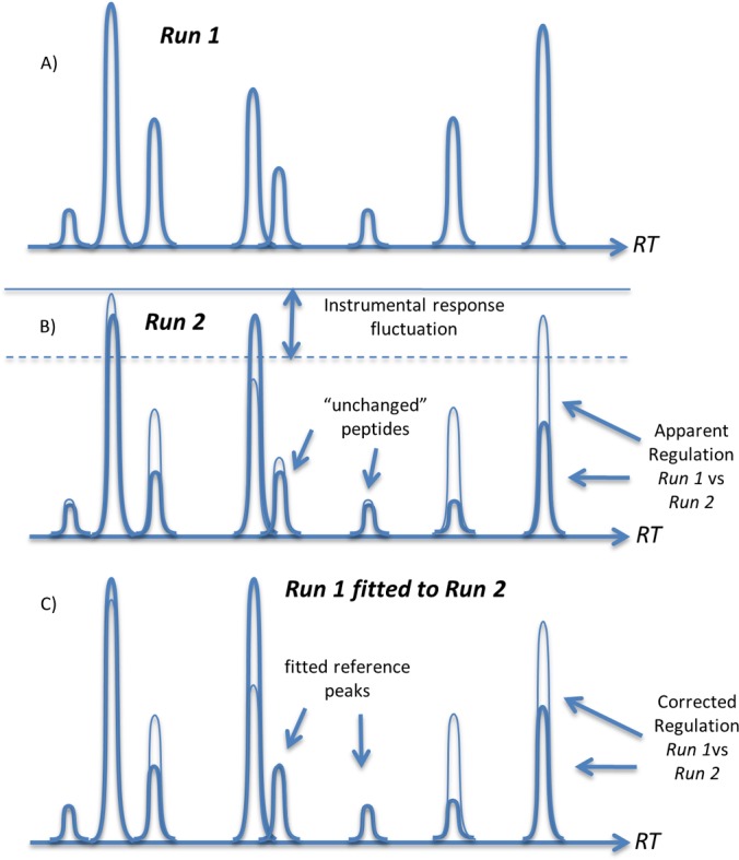
The principle of instrumental response correction using alignment of two LC-MS/MS runs. A, an RT window contains several peptide chromatographic peaks eluting within this window (for clarity, no overlap on the RT scale is shown). B, some of the peaks correspond to unchanged peptides that can be identified via statistical methods. C, these unchanged peaks are used to normalize the abundances of all peptides in run 1, which provides corrected ratios with respect to their abundances in run 1.

Our method of instrumental response correction is computationally inexpensive and fast (seconds for a pair of LC-MS runs). The ease of the method and its generality might earn it widespread application in proteomics, metabolomics, and other LC-MS/MS-related techniques.

MATERIALS AND METHODS

Proteomics Experiment

218 blood plasma samples from the Kuopio cohort were obtained in the course of the EU 7th Framework Programme's project PredictAD. This project defines long-term goals of research, order and procedure of scientific collaboration, and possible ethical issues related to the scientific activity. Detailed descriptions of sample collection and preparation, clinical considerations, and procedures are available in articles published in the context of this project (11). Only the information limited to sex, age, and state of Alzheimer disease was available for the samples. The provided samples were pooled according to gender and the stage of Alzheimer disease (control, mild cognitive impairment, progressive mild cognitive impairment, and Alzheimer disease). Each pooled sample was independently digested in triplicate by trypsin in ProteaseMAX™ Surfactant, Trypsin Enhancer (Promega, Madison, WI) according to the protocol provided by the producer. Each individual sample was digested once using the same protocol. Each peptide digest of pooled samples was analyzed twice using nanoflow C18 reverse-phase liquid chromatography (HPLC) (Easy-nLC, Proxeon, Odense, Denmark) with a 60-min gradient coupled with electron transfer dissociation MS/MS on a Velos Orbitrap mass spectrometer (Thermo Fisher Scientific). Survey MS scans were carried out in the Orbitrap Fourier transform mass analyzer with a resolution of 60,000, with the m/z ranging from 300 to 2000. After each MS scan, the top five most abundant precursor ions were selected for MS/MS using high-energy collision dissociation in the Orbitrap (resolution of 7500) and electron transfer dissociation in the Velos ion trap. Each of the individual samples was analyzed once using the same conditions as above, but with a nanoAcquity UPLC (Waters, Milford, MA) and using a shorter, 30-min-long gradient. Individual samples were analyzed in two uninterrupted series of LC-MS/MS runs with a three-week break between the series. For the current study, samples of 19 healthy males and 16 healthy females 71 ± 6 years old were selected representing LC-MS/MS runs from both series.

Peak List Generation and Database Search

MS/MS spectra were extracted using the home-written program RAW_to_MGF v. 2.0.5, which selected the 200 most intense peaks for each MS/MS spectrum and also cleaned electron transfer dissociation MS/MS spectra from precursors and neutral losses according to Ref. 12. Then, MS/MS spectra from different runs were clustered together using the home-written program Cluster_to_MGF v 2.0.6 to make a single .mgf file for pooled samples and two .mgf files for individual samples before and after the break, respectively. Cluster_to_MGF gathers groups of spectra that are presumed to be of the same compound. Spectra are included in this group if they share 10 of the 20 most intense peaks with at least one other spectrum in group. One spectrum from each group with the maximum aggregate intensity is taken as representative of this group for aggregation in the .mgf file.

The resultant .mgf files were searched using Mascot v. 2.3 (Matrix Science, London, UK) using high-energy collision dissociation and electron transfer dissociation data, with a precursor mass accuracy of 10 ppm, MS/MS accuracy of 0.6 Da, a maximum of two missed cleavages, carbamidomethylation of cysteine as a fixed modification, and asparagine and glutamine deamidation and methionine oxidation as variable modifications (the inclusion of these variable modifications makes sequence assignment more reliable). The database search was performed against the IPI Human V3.86 database concatenated with a decoy reverse-sequence compilation of this database for false discovery rate determination (contains 183,042 sequences, 91,521 of which are reversed). 1455 unique peptides belonging to 157 proteins were identified in the pooled samples with a false discovery rate of <1% (spectra peptide assignment was treated as false positive if its best hit matched in the database a reversed protein sequence). Before and after the break, 785 and 1109 peptides and 130 and 149 proteins were identified, respectively, in individual samples (supplemental Data S2). The Mascot score threshold required in order to keep a 0.01 false discovery level for accepting individual MS/MS spectra was 30.68 for pooled samples and 34.04 and 32.01, respectively, for individual samples before and after the break.

Quantification of the proteins was performed using the home-written program Quanti v. 2.5.2.1. This program performs the label-free extracted-ion-chromatogram-based quantification of peptides presented in Mascot search results considering all available isotopes and charge states. Quanti uses for quantification only reliably identified (false discover rate < 0.01), first-choice, unmodified, unique-sequence peptides. No fewer than two such peptides have to be present in order for a protein to be quantified. For each protein, one of the database I.D.s was selected that covered all the identified peptide sequences for that protein. All the I.D.s corresponding to the same peptide set or subset of that peptide set were also cited (supplemental Data S4). If two database protein entries had partial intersection, then all the peptides belonging to that intersection were excluded from the analysis.

This method yielded 105 quantified proteins in pooled samples, with 72 and 93 quantified proteins in individual samples before and after the break, respectively, excluding 4 keratin proteins that showed large sample-to-sample variation and were attributed to contamination.

Abundance alignment was implemented as part of the Quanti program. A single alignment step between two LC-MS/MS runs representing case and control consisted of the following steps:

1. Simultaneous label-free quantification analysis of all LC-MS/MS runs, including the alignment of peptides' retention times (RTs), and a determination for each peptide in each LC-MS/MS run of the RT and abundance A (integral of the extracted chromatographic peak of the peptide ion, including all isotopes and charge states). Fig. 2A shows the total ion chromatograms of two consecutive LC-MS/MS runs of the same digest. The total ion chromatogram variation between the runs is chiefly due to the fluctuation of the instrumental response function.

2. Despite the apparently reasonable overlap between the total ion chromatogram traces in Fig. 2A, detailed analysis showed that the peptide abundances in the two LC-MS/MS runs varied quite significantly. The smoothed ratios r of the same-peptide abundances are shown in Fig. 2B. The nonrandom component of r apparently drifts on the minute time scale and, in this particular example, reached a magnitude of 50% or more. Despite such strong fluctuations of the instrumental response, the correlation plot for peptide abundances between these two runs still gave a decent R² ≈ 0.97 (supplemental data). This value could be considered acceptable in today's proteomics, and thus the large systematic, time-dependent drift of relative peptide abundances could easily be overlooked in routine proteomics experiments.

3. To eliminate or drastically reduce the above-mentioned fluctuation, a sliding window ΔRT was arranged centered on a peptide of interest (all peptides were chosen in consecutive RT order). The width of ΔRT can be adjusted from seconds to minutes, but in general it should be larger than the typical width of a chromatographic peak. Shorter windows closely follow rapid fluctuations in the ESI current, but can result in misidentification of the unchanged peptides.

   Within each ΔRT window, the r values of all peptides eluting within that window were sorted in ascending order, and the median value of r was selected (Fig. 2C). In the selection of the median, peptide abundances can be taken into account to discriminate against the low-abundant peptides, whose abundances are measured less precisely. Empirically, we determined that the square root of the peptide abundance provides an optimal weighting factor for the median calculations.

   Peptides that are best avoided for median calculations are those that may originate from in vitro post-translational modifications of tryptic peptides, such as deamidated analogues of peptides with Asn and Gln residues and oxidized Met residues. The abundance of these modified species can vary significantly even in technical replicates depending upon minute details of sample handling, storage, and the order of sample injection.

4. Median case/control values for all ΔRT windows were smoothed using the same window width for smoothing as was used to get median peptide ratio values. The spectrum of the smoothed corrected values plotted against the RT (similar to Fig. 2B) can be used for quality control. Smoothed median values were then used as RT-dependent correction factors (Fig. 1B; each peptide abundance in run 2 was divided by the corresponding correction factor). After correction, R² for the two runs in Fig. 2A improved to 0.997.

5. Protein regulation factors were calculated as medians of the corrected ratios of the unique peptides composing the protein. If there are more than two samples in an experiment, matrix A is created for each protein, such that each element a_ij is the ratio of the abundances v_k in a pairwise comparison of the ith and jth samples: a_ij = v_i/v_j. The matrix A is reciprocal (a_ij = 1/a_ji), but it is inconsistent (a_ik ≠ a_ij*a_jk) because of the independent calculation of a_ij, a_jk, and a_ik. The theory of using reciprocal inconsistent matrices for approximating true abundance ratios was developed in the late 1970s by Saaty and colleagues (13). The best estimate of the true relative protein abundance of the jth protein is the geometric mean of a_1j to a_nj. (14). There is a simple explanation for why the geometric mean is better suited in this case than an arithmetic average: the a_ij ratios are asymmetric entities, with the up-regulation range being a = (1, ∞) and a down-regulation range of (0, 1). Therefore, the arithmetic mean gives a biased estimate. At the same time, log(a) is symmetric within the ranges (−∞, 0) and (0, ∞), and thus the arithmetic average of the logarithms of ratios (which is equivalent to a geometric average of ratios) is unbiased.

Fig. 2.

A, total ion chromatograms of two consecutive LC-MS/MS runs of the same proteomics sample (technical replicates). B, the median ratios r of the abundances of the same peptides eluting within a ±1 min RT window in the two runs. In the absence of the instrumental response fluctuations, the expected value is unity for all peptides. C, the ratios r are sorted according to their value; a median is calculated using the square root of the peptide abundance as a weight factor.

In principle, the correction method improves only the measurement precision. It is known in statistics that any manipulation of data, including any kind of normalization, can only reduce the accuracy (deviation of the result from the true value) and can never improve it. However, normalization that reduces the accuracy less than it improves the precision can have a huge beneficial effect on the statistical power (e.g. reduce the number of replicate analyses necessary to detect statistically significant changes in protein abundances, as discussed above). Thus a normalization method that slightly reduces the accuracy (e.g. produces an 18% difference instead of the true value of 20%) but significantly improves the precision and thus greatly reduces the number of experiments can be very valuable in practical terms.

RESULTS AND DISCUSSION

Precision Improvement

Fig. 3 demonstrates the significant improvement in the CV after the ESI current alignment procedure. Starting from proteins with five quantified peptides, the average CV is below 5%, whereas for proteins with ≥10 peptides, the CV is below 3%. The lowest CV of ≈1% was obtained for proteins with ∼100 peptides. This value represents the intrinsic precision of the alignment method: as is true of every post-processing correction, it can lead to marked improvement only when the instrumental response fluctuations are significant. Therefore, it is advisable to analyze the data with and without the correction, choosing the approach that produces lower CVs for a particular dataset.

Fig. 3.

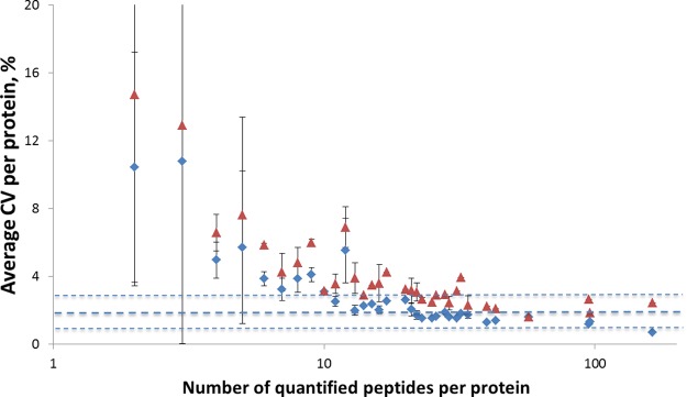
The average CV of proteins in analyzed human blood plasma as a function of the number of unique peptides quantified per protein before (red triangles) and after (blue diamonds) instrumental response correction.

These CV improvements represent an intermediate result; the real aim of the correction is to reduce the p value characterizing the difference between biologically distinct samples. Below, we provide an example of measuring such a difference as the ultimate test for the utility of the correction method.

Sex Differentiation

Abundant proteins in human blood are found in varying concentrations, and their relative abundances change in response to changing conditions (15). It has been known since the 1960s that alpha2-macoglobulin, the third most abundant protein in blood plasma, is present in adult female samples at an approximately 15% higher concentration than in adult male samples (16). We decided to look for sex differences among 70 to 100 of the most abundant proteins, because there are only a few reports in the literature of studies on sex differentiation via proteomics blood analysis (17, 18), none of which used label-free quantification. The working hypothesis was that, because protein biomarkers often show sex differences in expression levels (17), many abundant proteins will show sex-specific differences, and using these it will be possible to build a model for sex differentiation. The accuracy of such a model built using proteomics data before and after the instrumental response correction will serve as a test of the utility of our method.

To create a predictive model for sex differentiation, all 105 proteins quantified within the 48 pooled samples (2 sex * 4 disease state * 3 digestions * 2 replicates) were correlated with the sex of the subjects, and the N most correlating and N most anti-correlating proteins were selected. For each sample, the relative abundances of positively and negatively correlating proteins were separately summed, and then the sum for anti-correlating proteins was subtracted from the positively correlating sum. A positive resulting value predicted female sex; negative values indicated male. The 24 obtained predictions for female samples and 24 male samples were then submitted to a two-tailed Student t test, yielding the p values presented in Fig. 4. It is clear that for a broad range of values (3 ≤ N ≤ 20), and especially for n = 8 to 15, the instrument response correction produced significantly lower p values (i.e. better sex separation). Whereas in standard-based multiple reaction monitoring the use of fewer analytes is clearly advantageous in terms of the analysis cost, there is no penalty for using as many proteins as desired to create a predictive model in the label-free analysis scheme. Therefore, we chose for our model n = 10 (i.e. 20 in total) proteins out of the quantified 105 proteins that could be found in both pooled and individual datasets (Table I). The instrumental response correction reduced the sample-to-sample variation of the same-sex model predictions (Table I, supplemental Fig. S1) and increased the “sex gap” between female and male predictions, ensuring 100% accuracy of that model (not surprising, given that it was built on pooled samples).

Fig. 4.

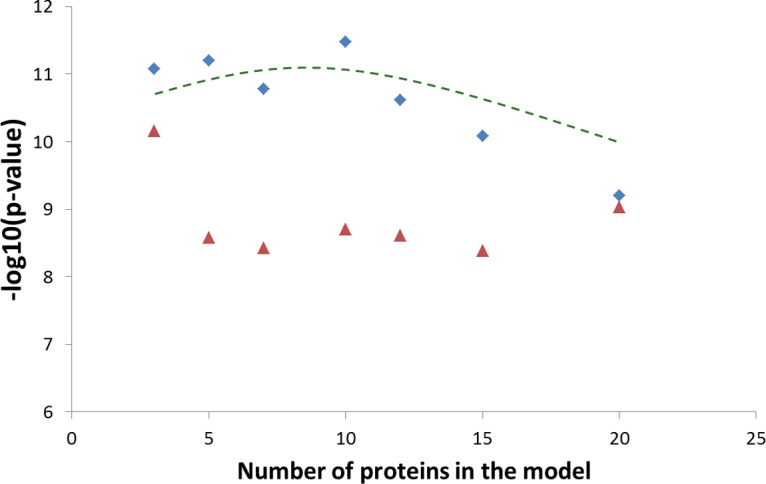
For each 24 pooled female and 24 pooled male blood plasma samples, the relative abundances of positively and negatively correlating with sex proteins were separately summed, and then the sum for anti-correlating proteins was subtracted from the positively correlating sum. The 24 obtained predictions for female samples and 24 for male samples were then subjected to a two-tailed Student's t test. The resultant p values before (red triangles) and after (blue diamonds) instrumental response correction are presented in the plot as a function of the number of proteins used for prediction.

Table I. The relative abundance ratios (male/female) and their standard errors for blood plasma proteins characteristic for females (upper part) and males (lower part) and used in the sex-differentiating model.

Protein I.D.	Protein name	Number of peptides	Not corrected, pooled	Corrected, pooled	Not corrected, individual	Corrected, individual
IPI01010737	A2M 165 kDa protein	58	0.755 ± 0.015	0.824 ± 0.017	0.87 ± 0.11	0.88 ± 0.09
IPI00896380	IGHM isoform 2 of Ig mu chain C region	14	0.728 ± 0.039	0.792 ± 0.033	0.79 ± 0.14	0.76 ± 0.13
IPI00021842	APOE apolipoprotein E	11	0.822 ± 0.017	0.915 ± 0.014	0.95 ± 0.17	0.93 ± 0.11
IPI00020986	LUM lumican	2	0.843 ± 0.021	0.884 ± 0.020	0.86 ± 0.11	0.85 ± 0.09
IPI00019943	AFM afamin	8	0.854 ± 0.019	0.915 ± 0.015	1.11 ± 0.09	1.08 ± 0.07
IPI00657670	APOC3 apolipoprotein C-III variant 1	4	0.808 ± 0.024	0.880 ± 0.025	0.85 ± 0.22	0.87 ± 0.16
IPI00021856	APOC2 apolipoprotein C-II	4	0.846 ± 0.029	0.893 ± 0.024	0.92 ± 0.17	0.93 ± 0.14
IPI00017601	CP ceruloplasmin	18	0.897 ± 0.021	0.945 ± 0.016	1.08 ± 0.11	1.07 ± 0.06
IPI00879573	SERPIND1 heparin cofactor 2	7	0.872 ± 0.024	0.934 ± 0.020	1.18 ± 0.10	1.10 ± 0.07
IPI00021855	APOC1 apolipoprotein C-I	5	0.868 ± 0.029	0.936 ± 0.021	0.92 ± 0.09	0.93 ± 0.08
	Average protein regulation		0.829 ± 0.024	0.892 ± 0.020	0.95 ± 0.13	0.94 ± 0.10
IPI00022429	ORM1 alpha-1-acid glycoprotein 1	4	1.053 ± 0.029	1.127 ± 0.027	1.32 ± 0.19	1.29 ± 0.18
IPI00930442	IGHG4 putative uncharacterized protein DKFZp686M24218	2	1.384 ± 0.076	1.429 ± 0.069	1.76 ± 0.20	1.62 ± 0.19
IPI00844536	RBP4 uncharacterized protein	5	1.019 ± 0.025	1.119 ± 0.024	1.08 ± 0.11	1.11 ± 0.09
IPI00953689	AHSG alpha-2-HS-glycoprotein	6	1.022 ± 0.027	1.072 ± 0.014	1.11 ± 0.06	1.15 ± 0.06
IPI00298828	APOH beta-2-glycoprotein 1	9	0.951 ± 0.012	1.052 ± 0.010	1.08 ± 0.10	1.11 ± 0.06
IPI00553177	SERPINA1 isoform 1 of alpha-1-antitrypsin	31	0.993 ± 0.015	1.075 ± 0.013	1.08 ± 0.10	1.07 ± 0.07
IPI00847635	SERPINA3 isoform 1 of Alpha-1-antichymotrypsin	12	1.024 ± 0.016	1.087 ± 0.014	1.08 ± 0.16	1.05 ± 0.10
IPI00298971	VTN vitronectin	5	1.026 ± 0.014	1.086 ± 0.013	1.21 ± 0.09	1.23 ± 0.05
IPI00745872	ALB isoform 1 of serum albumin	79	1.011 ± 0.009	1.104 ± 0.008	1.03 ± 0.02	1.05 ± 0.03
IPI00607707	HPR isoform 2 of haptoglobin-related protein	2	1.420 ± 0.041	1.427 ± 0.028	1.55 ± 0.17	1.43 ± 0.15
	Average protein regulation		1.090 ± 0.026	1.158 ± 0.022	1.23 ± 0.12	1.21 ± 0.10

The same 20 best correlating and anti-correlating proteins from the pooled sample analysis were used for sex differentiation based on a single LC-MS/MS analysis of 16 individual female and 19 male blood samples. These blood samples were digested and run only once, using a different HPLC with a much shorter gradient (30 min versus 60 min), thus mimicking an independently made routine analysis performed in a high-throughput manner. This, as well as the three-week break between some of the runs (see above), makes this dataset a challenging but particularly realistic test object. Instrumental response correction reduced the standard error of the protein abundance measurement even for individual samples (Table I).

Without the correction (Fig. 5A), the model achieved 80% accuracy in sex identification, misclassifying 7 out of 35 samples. After the correction, only four samples were classified incorrectly, giving the classification an accuracy of approximately 90%. The p value of the difference between the sex groups improved from 5.0 × 10⁻² to 7.8 × 10⁻⁷. Note also that out of the three “bad” outliers in Fig. 5A, two are much closer to their true class in Fig. 5B. It is realistic to suggest that, using more technical replicates and perhaps two to three digestions per sample, one can achieve nearly 100% accuracy in sex differentiation through a rather “shallow” proteomics analysis.

Fig. 5.

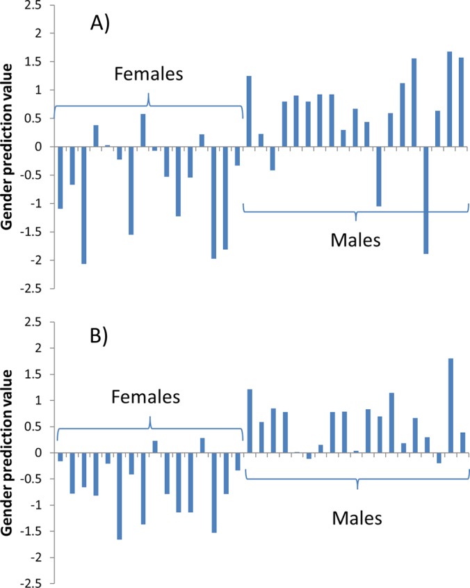
Sex classification based on a single LC-MS/MS run for 16 females and 19 males using the same 20-protein model as was obtained for the pooled blood plasma samples (Fig. 4), before (A) and after (B) instrumental response correction.

CONCLUSIONS

This new method of instrumental response correction significantly improves the precision of label-free proteomic quantification and increases the accuracy of predictive models based on the measurements. We have demonstrated that the accuracy of the sex differentiation model based on “one-shot” proteomics data is significantly improved upon application of the instrumental response correction. The correction method is general and, in principle, can be used for many proteomics and metabolomics datasets acquired in a label-free experiment. The off-line, post-processing character of our correction sets it apart from the on-line, real-time monitoring methods that reject experiments performed in deviating conditions (19). The method is built into versions 2.4 and higher of the in-house software Quanti operating with Thermo .raw files and available from the authors upon request. We have been using the above-described method in our laboratory for almost two years and have tested it thoroughly on hundreds of proteomics datasets.

REFERENCES

- 1. Bondarenko P. V., Chelius D., Shaler T. A. (2002) Identification and relative quantitation of protein mixtures by enzymatic digestion followed by capillary reversed-phase liquid chromatography-tandem mass spectrometry. Anal. Chem. 74, 4741–4749 [DOI] [PubMed] [Google Scholar]
- 2. Neilson K. A., Ali N. A., Muralidharan S., Mirzaei M., Mariani M., Assadourian G., Lee A., van Sluyter S. C., Haynes P. A. (2011) Less label, more free: approaches in label-free quantitative mass spectrometry. Proteomics 11, 535–553 [DOI] [PubMed] [Google Scholar]
- 3. Nunn B. L., Shaffer S. A., Scherl A., Gallis B., Wu M., Miller S. I., Goodlett D. R. (2006) Comparison of a Salmonella typhimurium proteome defined by shotgun proteomics directly on an LTQ-FT and by proteome pre-fractionation on an LCQ-DUO. Brief. Funct. Genomics Proteomics 5, 154–168 [DOI] [PubMed] [Google Scholar]
- 4. Xie F., Liu T., Qian W.-J., Petyuk V. A., Smith R. D. (2011) Liquid chromatography-mass spectrometry-based quantitative proteomics. J. Biol. Chem. 286, 25443–25449 [DOI] [PMC free article] [PubMed] [Google Scholar]
- 5. Blagoev B., Kratchmarova I., Ong S. E., Nielsen M., Foster L. J., Mann M. (2003) A proteomics strategy to elucidate functional protein-protein interactions applied to EGF signaling. Nat. Biotechnol. 21, 315–318 [DOI] [PubMed] [Google Scholar]
- 6. Ibarrola N., Kalume D. E., Gronborg M., Iwahori A., Pandey A. A. (2003) Proteomic approach for quantitation of phosphorylation using stable isotope labeling in cell culture. Anal. Chem. 75, 6043–6049 [DOI] [PubMed] [Google Scholar]
- 7. Juraschek R., Röllgen F. W. (1998) Pulsation phenomena during electrospray ionization. Int. J. Mass Spectrom. 177, 1–15 [Google Scholar]
- 8. Marginean I., Parvin L., Heffernan L., Vertes A. (2004) Flexing the electrified meniscus: the birth of a jet in electrosprays. Anal. Chem. 76, 4202–4207 [DOI] [PubMed] [Google Scholar]
- 9. Parvin L., Galicia M. C., Gauntt J. M., Carney L. M., Nguyen A. B., Park E., Heffernan L., Vertes A. (2005) Electrospray diagnostics by Fourier analysis of current oscillations and fast imaging. Anal. Chem. 77, 3908–3915 [DOI] [PubMed] [Google Scholar]
- 10. Constantopoulos T. L., Jackson G. S., Enke C. G. (1999) Effects of salt concentration on analyte response using electrospray ionization mass spectrometry. J. Am. Soc. Mass Spectrom. 10, 625–634 [DOI] [PubMed] [Google Scholar]
- 11. Julkunen V., Niskanen E., Koikkalainen J., Herukka S. K., Pihlajamäki M., Hallikainen M., Kivipelto M., Muehlboeck S., Evans A. C., Vanninen R., Soininen H. (2010) Differences in cortical thickness in healthy controls, subjects with mild cognitive impairment, and Alzheimer's disease patients: a longitudinal study. J. Alzheimers Dis. 21, 1141–1151 [DOI] [PubMed] [Google Scholar]
- 12. Good D. M., Wenger C. D., McAlister G. C., Bai D. L., Hunt D. F., Coon J. J. (2009) Post-acquisition ETD spectral processing for increased peptide identifications. J. Am. Soc. Mass Spectrom. 20, 1435–1440 [DOI] [PMC free article] [PubMed] [Google Scholar]
- 13. Saaty T. L. (1977) A scaling method for priorities in hierarchical structures. J. Math. Psychol. 15, 234–281 [Google Scholar]
- 14. De Jong P. A. (1984) Statistical approach to Saaty's scaling method for priorities. J. Math. Psychol. 28, 467–478 [Google Scholar]
- 15. Anderson N. L., Anderson N. G. (2002) The human plasma proteome: history, character, and diagnostic prospects. Mol. Cell. Proteomics 1, 845–867 [DOI] [PubMed] [Google Scholar]
- 16. Ganrot P. O., Schersten B. (1967) Serum a2-macroglobulin concentration and its variation with age and sex. Clin. Chim. Acta 15, 113–120 [Google Scholar]
- 17. De Torres J. P., Casanova C., Pinto-Plata V., Varo N., Restituto P., Cordoba-Lanus E., Baz-Dávila R., Aguirre-Jaime A., Celli B. R. (2011) Gender differences in plasma biomarker levels in a cohort of COPD patients: a pilot study. PLoS One 6, e16021. [DOI] [PMC free article] [PubMed] [Google Scholar]
- 18. Miike K., Aoki M., Yamashita R., Takegawa Y., Saya H., Miike T., Yamamura K. (2010) Proteome profiling reveals gender differences in the composition of human serum. Proteomics 10, 2678–2691 [DOI] [PubMed] [Google Scholar]
- 19. Scheltema R. A., Mann M. (2012) SprayQc: a real-time LC-MS/MS quality monitoring system to maximize uptime using off the shelf components. J. Proteome Res. 6, 3458–3466 [DOI] [PubMed] [Google Scholar]
Associated Data
This section collects any data citations, data availability statements, or supplementary materials included in this article.