Abstract
The relationship between a market index and its constituent stocks is complicated. While an index is a weighted average of its constituent stocks, when the investigated time scale is one day or longer the index has been found to have a stronger effect on the stocks than vice versa. We explore how this interaction changes in short time scales using high frequency data. Using a correlation-based analysis approach, we find that in short time scales stocks have a stronger influence on the index. These findings have implications for high frequency trading and suggest that the price of an index should be published on shorter time scales, as close as possible to those of the actual transaction time scale.
Understanding financial markets as complex adaptive systems1,2,3,4,5 is crucial in the light of the current world economic reality. The approach provides an important key to rethinking many failing economic theories heretofore considered axiomatic6. A prominent characteristic of complex systems is their display of emergent phenomena1,2. It has recently been suggested that a market index plays this role in a financial market7,8,9,10,11, that there is a special feedback loop between an index and its constituent stocks1, and that an index more strongly affects the stocks than the stocks affect the index. This raises several important questions. What is the source of market dynamics? Does a change in the index at time t cause a change in stock prices at time t + 1? Does a change in one stock of the index at time t cause a significant change in the index price at time t + 1? If so, does this change in the index price in turn cause changes in other stock prices in the index?
Many studies have shown that on a daily time horizon an index has a driving force, often referred to as the “leverage effect”7,8,9,11,12,13,14,15,16,17. Although this leverage effect is observable in low to medium frequency data, its existence in small time scales is still not clear. As a complex system, the dynamics of financial systems take place on many different time scales, and it is crucial to explore the underlying structure and dynamics in these different time scales. To get a fuller understanding of the relationship between a market index and its components, it is crucial to investigate this relationship on shorter time scales. In recent years the use of high frequency financial data has become increasingly popular18,19,20,21,22,23,24,25,26,27.
The U.S. Securities and Exchange Commission (SEC) authorized electronic exchanges in 1998, and since that time high-frequency trading (HFT) has become widespread. By the year 2001, HFT trades had an execution time of several seconds. By 2010 this had shrunk to milliseconds, even microseconds28. For a long time high-frequency trading was a little-known phenomenon outside the financial sector, but a July 2009 article in The New York Times was instrumental in bringing the subject to wider attention29. In the early 2000s, high-frequency trading accounted for less than 10% of equity orders, but this proportion grew rapidly. According to data from the NYSE, high-frequency trading volume grew by ≈ 164% between 2005 and 200929. In the first quarter of 2009 the assets under hedge fund management with high-frequency trading strategies totaled $141 billion, ≈ 21% less than the peak prior to the 2008 downturn30. The high-frequency strategy was first used successfully by Renaissance Technologies. Many high-frequency firms are market makers and provide the liquidity to the market that lowers volatility, helps narrow bid-offer spreads, and makes trading and investing cheaper for other market participants. In the United States, high-frequency trading firms represent 2% of the approximately 20,000 firms operating today, but account for 73% of the volume of all equity orders. The largest high-frequency trading firms in the US include such names as Getco LLC, Knight Capital Group, Jump Trading, and Citadel LLC. The Bank of England estimates similar percentages for the 2010 US market share, also suggesting that in Europe HFT accounts for about 40% of the volume of equity orders, and for Asia about 5–10%, with a high potential for rapid growth28. In terms of value, consultants in the Tabb Group estimated that HFT in 2010 constituted 56% of equity trades in the US and 38% in Europe31. HFT has recently been described as a major contributing factor in the 6 May 2010 “flash crash”32,33 and in the incident involving Knight Capital34.
Traders with access to high-frequency information receive updates in stock price changes at down to centi-second intervals. This gives them an extremely important advantage in the market, given that regular household traders usually receive updates on much slower time scales. In addition, while stocks are being traded on a centi-second time scale, the market index value is displayed on a time scale of several seconds—a time difference that provides a significant advantage to high-frequency traders. The high-frequency traders can execute trades within the longer time intervals during which the index is calculated, and thus affect the index, which in turn will affect other stocks.
Our goal is to investigate the relationship between market index and stock prices in time scales that are shorter than the update intervals of an index. We want to determine whether the change in an index influences the stocks, or the changes in stock prices influence an index. In our approach to this question, we use the high-frequency trading data of stocks making up the Tel-Aviv 25 (TA25) Index, and construct a synthetic index, calculated in time scales shorter than the 30-second time scale of the TA25 Index. We then compare the two indices and study their cross correlations in order to test whether the change in the price of the stocks is more correlated to the change of the market index, or to that of the stocks themselves. In addition, we use influence analysis, a recently developed tool, to study which of the two indices has a stronger effect on stock price correlations.
Results
Synthetic index versus market index
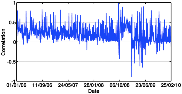
We begin by constructing the time series for the two indices, the TA25 Index and our synthetic index. Both indices are made up of 1025 days with 1681 time records of 15-second intervals for each day. Figure 1 shows the correlation between the synthetic index and the market index, calculated for each day. To investigate the relationship between the two indices, we use cross-correlation analysis (see Methods). We first determine the average sample cross correlation function (XCF) as a function of the lag. The averaging is done across all the days in each of the three groups.
Figure 1. Daily correlation between the synthetic index and the market index.
We investigate the average XCF values using a box-plot analysis. The box-and-whisker diagram35 graphically depicts groups of numerical data through their five number summaries: the smallest observation (sample minimum), lower quartile (Q1), median (Q2), upper quartile (Q3), and largest observation (sample maximum). A box-plot may also indicate which observations, if any, might be considered outliers. Box-plots display differences between populations without making any assumptions about the underlying statistical distributions: they are nonparametric. The spacings between the different parts of the box help indicate the degree of dispersion (spread) and skewness in the data, and they identify outliers. In this representation, the bottom-most vertical line represents the minimum of the sample, and the upper-most vertical line represents the maximum of the sample. The bottom of the box represents the 25th percentile, and the top of the box the 75th percentile, with the line inside the box representing the 50th percentile, which is the median. In this way it is possible to present both the median and the entire spread of the sample population.
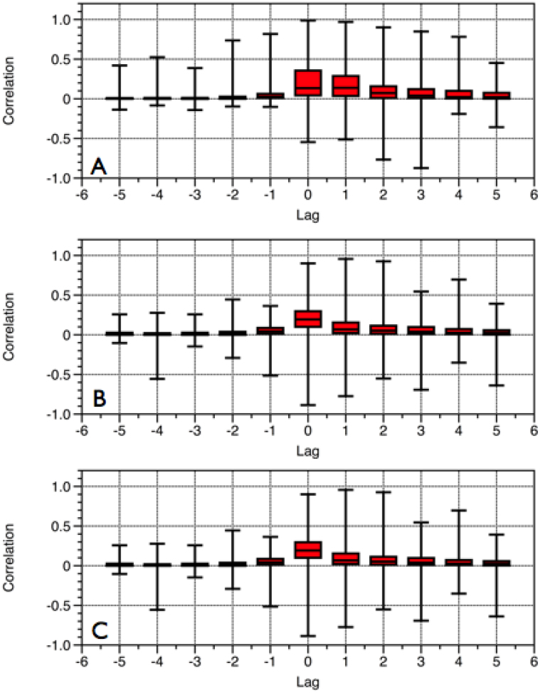
Using the box-plot representation in Fig. 2, we find that the correlation values for Lag = +1 have a median and a STD for all three groups that is larger than those for Lag = −1. Note that the minimum value and the top of the box are both very close to zero and thus for the medium and high group (Fig. 2B and Fig. 2C respectively) most of the values of the correlation are near zero. Note also that in the high group the values in the 25th to 75th percentile range for Lag = +1 are larger than those for Lag = −1. We also see that these values are larger for Lag = +3 than for Lag = +2, which again indicates that there is more information in the synthetic index than in the market index. Table I shows the average XCF value calculated for Lag = ±1 for the three groups. We find that the distribution of the values for the lags larger than zero is much wider than for the values of the lags smaller than zero (see Figure 2). To test this observation, we calculate the range of the values in terms of the maximal value minus the minimal value, and calculate the ratio between the range for the corresponding lag above zero and below zero, which gives the spread ratio,
 |
We first calculate the ratio between the range for the Lag = −1 values and then divide this range by the range of the Lag = +1 values. Table II shows the spread ratio values. The range of the correlation values for positive lags are always larger than those for negative lags. For all three groups, we observe that the range of the positive lags is larger by 30 to 80 percent than that of the negative lags (we see this when looking at one minus the values presented in Table II).
Figure 2. Box-plot representation of the XCF, as function of the lag, for the (A) low, (B) medium, and (C) high STD groups, as categorized by the second classification rule.
The bottommost vertical line represents the minimum of the sample, the bottom line of the box represents the 25th percentile, the line inside the box represents the median, the uppermost line of the box represents the 75th percentile, and the topmost vertical line represents the maximum of the sample.
Table 1. Average XCF values. Average value of XCF, calculated for a lag of plus/minus one, for the three groups.
| Group | Lag = +1 | Lag = −1 |
|---|---|---|
| Low | 0.1868 | 0.0600 |
| Medium | 0.0944 | 0.0548 |
| High | 0.094 | 0.0548 |
Table 2. Values of the spread ratio, for the three groups.
| N | Low | Medium | High |
|---|---|---|---|
| 1 | 0.6196 | 0.5081 | 0.5081 |
| 2 | 0.4996 | 0.4986 | 0.4986 |
| 3 | 0.3074 | 0.3268 | 0.3268 |
| 4 | 0.6260 | 0.7941 | 0.7941 |
| 5 | 0.6874 | 0.3501 | 0.3501 |
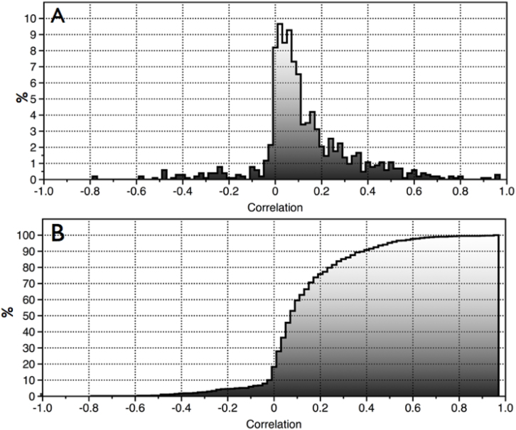
To determine the correlation values for Lag = +1 for all days, we study the histogram of these 1025 values (corresponding to the 1025 days in the analysis). Figure 3 shows the histogram in which the y-axis is the percentage out of the whole for a given bin. We see that the distribution of values is asymmetric, with a long tail and higher probability for positive values. Figure 3B shows the commutative distribution function (CDF). We see that 90% of the correlation values for Lag = +1 are > 0 and 10% of the values (102 days) are > 0.4, a significantly high correlation value. We note that 1% of the total period (12 days) have correlation values > 0.7, and 0.7% (7 days) have correlation values > 0.8.
Figure 3. Correlation values for Lag = + 1 for 1025 days.
In panel A we present the histogram of the values, where the y-axis represents the percentage out of the whole for the value in each bin. This clearly shows that there is a higher probability for positive correlationvalues. In panel B we present the commutative distribution function (CDF) of values. The CDF shoes that 90% of the days have positive correlation values for this lag, 10% of the days (n = 102) have correlation >0.4, 1% of the days (n = 12) have correlation >0.7, and 0.7% of the days (n = 7) have correlation >0.8.
Market index versus synthetic index in different years
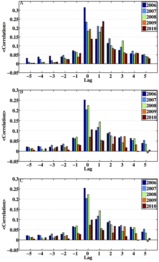
We repeat the above analysis on a year-by-year basis. There were 40 trading days for 2010, and 245 for all other years. Figure 4 shows the average XCF as a function of lag calculated for individual years. We see that the average XCF at lag zero for all three groups was larger for the years 2006–2008. This is most obvious in the medium and large STD groups in which the average XCF at lag zero in 2006–2008 is more then twice as high as in 2009. Note also that for the medium and large STD groups the average XCF at Lag = +1 was almost twice as large as that at Lag = −1 in 2006–2008, but that they were almost the same in 2009. Both of these findings indicate that the dynamics of the market was sharply different in 2009. This was probably the result of the strong positive trend in the market as it recovered from the 2008 financial crisis. Note that the average XCF values differ significantly in 2010. While it is plausible that the relationship between the stocks and the index changed in 2010 as a result of the change in the macro and microeconomic conditions, the data for 2010 encompasses only 40 days, too little to allow any clear conclusions.
Figure 4. Average XCF, as function of lag, for each year separately.
The average is calculated over days categorized into the low (A), medium (B), and high (C) STD.
Table III shows the average XCF for Lag = +1 and Lag = −1 for each year. As was the case in Table I, we see that in the Equal category the low group has the higher average XCF values.
Table 3. Average value of XCF, calculated for a lag of plus/minus one, for the three groups, computed separately for each year.
| 2006 | 2007 | 2008 | 2009 | 2010 | ||||||
|---|---|---|---|---|---|---|---|---|---|---|
| Group | +1 | −1 | +1 | −1 | +1 | −1 | +1 | −1 | +1 | −1 |
| Low | 0.1385 | 0.0737 | 0.2099 | 0.0684 | 0.1770 | 0.0637 | 0.2067 | 0.0380 | 0.2373 | 0.0585 |
| Medium | 0.1025 | 0.0656 | 0.1169 | 0.0614 | 0.1437 | 0.0696 | 0.0539 | 0.0327 | 0.0510 | 0.0295 |
| High | 0.1013 | 0.0661 | 0.1169 | 0.0614 | 0.1431 | 0.069 | 0.0558 | 0.0326 | 0.0471 | 0.0273 |
Index influence analysis
We make further use of partial correlation influence analysis36,37,38 to determine which index has the greater impact on stock correlations. Using the market index and the synthetic index, we compare their influence on individual stock correlations (see Supplementary Information A). We do this as follows:
We construct the synthetic index and the market index at 15-second intervals for each day.
We compute the correlation matrix of all the stocks participating in the index for that day (ranging from 25 to 28) and add the time series of the synthetic index and the market index. Thus, if for a given day there are 25 stocks in the index, then the two indices and the resulting matrix is a 27 × 27 correlation matrix.
We use partial correlation influence analysis to compute how many correlations each stock affects.
We use the system level influence score to calculate, for each stock and for the two indices, the number of stocks affected by each index.
For each day, we calculate the ratio between the number of stocks the synthetic index influences and the number of stocks the market index influences. This give us the index influence (II) ratio,
 where t is a given day.
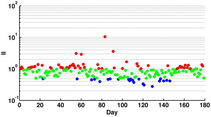
Out of the 1025 days in the sample, we found 179 days in which the indices had a nonzero influence on other stocks. The low percentage of days with nonzero influence for this threshold suggests that the correlations were rather homogeneous for the remaining days in the studied period. In Figure 5 we present a semi-logarithmic plot of the II values for days with nonzero influence. We divided the values into three groups: values of II smaller or equal to 0.5 - blue; values of II larger than 0.5 or smaller or equal to 1 - green; and values of II larger than 1 - red. The blue circles represent days in which the market index had a stronger influence on the stocks correlations. The green circles correspond to days in which the influence of the synthetic index and the market index were roughly the same. Finally, the red circles correspond to days in which the synthetic index had a stronger influence on stock correlations. We expect a priori that both indices should have a similar affect on the stock correlations, thus all days should be green. However, looking at Fig. 5, we find that this is not the case.
Figure 5. We calculate the ratio between the number of stocks influenced by the synthetic index and the number of stocks influenced by the market index.
The x-axis is days in which there was a nonzero influence, and the y-axis is the value of the II, in a logarithmic scale. The days are color-coded: blue, II ≤ 0.5; green, 0.5 < II ≤ 1.0; and red, II > 1.0.
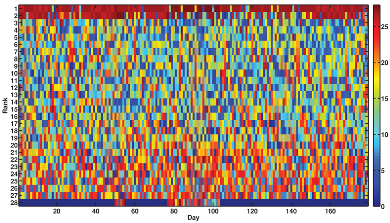
Finally, for each day with a nonzero influence, we rank each stock according to the number of stocks it influences. We then sort all stocks according to their rank. Figure 6 shows the result of this ranking process, with the x-axis representing days and the y-axis rank. The color of each cell indicates the number of the stock. Because the stocks included in the analysis are not constant across time, the same number (color) can refer to different stocks on different days, but the two indices are always represented by the two darkest shades of red. Note that the most influential on most days is the market index. For a small number of days the other index, usually the synthetic index, is the second most influential. Note also that there are a very few days in which neither the market index nor the synthetic index are among the top two most-influential stocks.
Figure 6. Ranking of stocks and indices, according to their influence, for each day.
The color represents the number of the stock/index, where for the majority of the days there were 25 stocks, and then the synthetic index was number 26, and the market index was 27. For a small percentage of the days, there were 26 stocks, and then the indices were numbered 27 and 28, respectively.
Discussion
Our goal in this research is to investigate a basic question in the underlying dynamics of financial markets: does a market index drive its constituent stocks, or vice versa? It has been found that on a daily time scale, an index has a stronger influence on its constituent stocks than the other way around1, but does this relationship change for shorter time scales? Over the past decade the use of sophisticated high-frequency trading has become widespread. In most modern financial markets stocks are traded at a centi-second (or smaller) time scale, but indices are published on longer time scales, usually several seconds. During the investigated time period in this work, the flagship index of the Tel-Aviv (TA) stock market, TA25, was published every 30 seconds. During this 30-second period, high frequency traders could potentially predict, or even affect, the next value of the index–and thus enjoy a significant advantage over other traders.
When we make use of a lag of one time record, we find that the average correlation calculated between the synthetic index and the market index over all trading days is higher than when we use a lag of minus one time record. If we fix the synthetic index and move the market index by one time record (15 seconds here), the synthetic index will correlate with the value of the market index at time t + 1. Thus when t = 15 seconds, the stocks have a greater influence on the index than vice versa.
In order to determine the nature of the stock-index relationship, we have focused on the average correlation values for different lags, and furthermore examine the distribution of the values. Figure 3 shows a histogram of the correlation values for all three groups for all 1025 days for a lag of plus one time record. Note that despite the relatively low average values, there are days when the correlation between the synthetic index and the market index is extremely high. Figure 3B shows the CDF of the values, and we observe that there are days when the correlation at lag of plus one is extremely high, e.g., the 12 days when the correlation is > 0.7, indicating that there are days when the high frequency trading of the stocks can possibly strongly impact the market index.
When we study each of the four years separately, we find that the results for each year of the 2006–2008 period are qualitatively similar to those found for the entire period. In 2009, however, we find a significantly smaller correlation. This could be the result of high frequency trading and other sophisticated trading mechanisms responding to the financial crisis during this period, but this is still unclear. An added factor during this chaotic period were the various governmental investigations into how high frequency trading was affecting market stability, e.g., the SEC investigation in the US and the European Commission in the EU. The low correlation observed in 2009 might also be the result of macroeconomic factors external to the market affecting stock price dynamics, such as the effect of various media on the spread of both accurate and inaccurate information.
In conclusion, this paper presents a high frequency analysis of the relationship between an index and its constituent stocks. Our results show that in short time scales the influence of stocks is stronger than the influence of the index. The stocks in the Tel-Aviv 25 (TA25) market are traded on a centi-second time scale, whereas the index is published on a time scale of seconds. High frequency players can thus take advantage of this difference in time scales and manipulate the market. One way to deal with the issue is to publish the index price more frequently, e.g, every second. Alternatively, this issue can be resolved by introducing limitations on the frequency of trading (e.g. by means of transaction fees, order fees, limit of number of allowed orders, etc.) to that of the publication of the index. In the future we plan to study how a very short time scale affects the relationships between stocks, and between the stocks and the index. It is possible that the relationship between the stocks and the index will change if the time between two consecutive publications of the index price is shortened. Furthermore, a natural continuation of this work would be to repeat the analysis using data from the order book itself. The results presented here sheds new empirical light on how a market index and its stocks are interdependent over very short time scales, and how high frequency trading affects the market.
Methods
Data
For this study, we use high frequency data of all stocks belonging to the Tel-Aviv 25 (TA25) Index, during the period January 2006 - February 2010, which is made up of 1025 trading days. The exact presence and impact of high frequency trading (HFT) in Israel is being carefully investigated by the different regulatory bodies in Israel, it is known that at least 6 major HFT companies operate in Israel, and that it's percentage of overall trading is constantly growing, on a year-by-year basis.
The TA25 index is the flagship index of the Tel-Aviv Stock Exchange (TASE), and is made up by the 25 largest companies in term of market cap. The makeup of the index is updated twice a year, on the 15 of June and December. The main index products available to trade the TA25 are Exchange Traded Notes (ETN), which are a senior, unsecured, unsubordinated debt security issued by an underwriting bank. Similar to other debt securities, ETN's have a maturity date and are backed only by the credit of the issuer. ETN's are designed to provide investors access to the returns of various market benchmarks. The returns of ETN's are usually linked to the performance of a market benchmark or strategy, less investor fees. When an investor buys an ETN, the underwriting bank promises to pay the amount reflected in the index, minus fees upon maturity (for more information, see39). The number of TA25 ETN's grew from one in 2006 to sixteen in 2010, and their percentage of market share has been growing on a year by year basis, and is estimated to have been at a level of 7% in the beginning of 2010.
During this period, 36 different stocks belonged to the TA25 Index, resulting from the fact that its makeup is updated every 6 months (total of 8 times for the investigated time period). The data for each stock included the following variables: date, time of transaction, open price, base price, close price, volume in units, trade stage, index intra-day value, index base price, and the index open price. The number of transactions per day varied between the different stocks, and ranged from Ntrans ~ 100 for stocks with low liquidity, to Ntrans ~ 2500 for stocks with high liquidity.
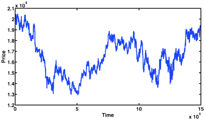
In this study we use the date, time, trade stage, open price, and index inter-day value. We remove all transactions carried out in the pre-hour trading (stage 2) and after hours trading (stage 4) stages of the trading day, and analyze only those transactions that take place in the continuous stage of trading (stage 3). Figure 7 presents an example of the price time series for all transactions of the stock of the Israeli company Teva, for the period 2006–2010.
Figure 7. Interday price change of TEVA for the trade period 2006–2010.
The time axis (x-axis) is time in the sense of transactions, starting from 1.0 at the beginning of the continuous trade stage for the first trading day (01/01/2006) until the end of the continuous trade stage of the last trading day (31/12/2009).
Synthetic index and market index
To study the relationship between the market index and the stocks, we create a synthetic index, which is calculated on shorter time scales than the market index. Since the market index was calculated every 30 seconds during the investigated time period, we set out to create a synthetic index which is calculated in a time interval shorter than 30 seconds. Thus, we chose to work with a 15-second time interval. First, we processed the raw data for each stock, so that for each day we have a price record every 15 seconds. The time of day studied was from 10:00 in the morning till 17:00 in the afternoon (which is the continuous trade stage). Starting at 10:00, we recorded the price of a given stock every 15 seconds. The price closest to the 15 second interval was used (instead of simply using the last price in the time interval, it is also possible to use the average of prices inside the interval; however, this did not lead to any significant changes in the results). If there was no price change inside the interval, the previous recorded price was used. This resulted in a time series of 1681 records, for every stock, for every day. Next, we transformed the processed data from price to return, using the commonly used transformation
where Pi(t) is the price of stock i at time t, and Δt is the sampling time resolution. We construct the 15-second synthetic index using the 15-second returns of each stock. This is done using the listing of the companies belonging to the TA25 index for the studied period (see Supplementary Information B). For each day, we only choose the stocks belonging to the TA25 index. We then make use of the information about their weight in the index, and use these weights to construct the synthetic index.
Finally, we process the data for the market index for the 15 second time resolution. As the time stamp in the data was set according to stock transactions, there were inconsistencies between the different stocks regarding the intraday price of the index. Thus, after processing the stock data into 15-second time intervals, we use the price of the index recorded for that given stock for the specific time record. We then average over all stocks belonging to the market index. Thus we construct a 15-second record index out of the 30-second market index.
Cross-correlation analysis
We perform a cross-correlation analysis between the synthetic index and the market index in order to study their similarity, keeping the synthetic index fixed and sliding the market index using different lags. Cross-correlation is a standard method in signal processing of estimating the degree to which two series are correlated (see for example40,41,42,43,44,45,46,47). The discrete cross-correlation function between two time series X and Y is given by48
 |
where d is the lag used. In this work we use values of d = ±1, ±2, ±3, ±4, ±5. For example, when we use the lag d = +1 to study the cross-correlation between the synthetic index and the market index the market index is shifted by one time point, which corresponds to 15 seconds. This way we study how the synthetic index return is correlated to the market index return, 15 seconds forward in time.
To calculate the cross correlation between the two indices, we divide the entire period (1025 days in this study) into three groups. We group the days based on the volatility of the synthetic index (in this case the standard deviation, STD). We first order all σ(i) according to their value, from smallest to largest. We next divide this ordered list into three equal groups–the first third are the low group, the second third are the medium group, and the last third are the high group. The number of days is equally divided among the three groups–341 days in the low group, 342 days in the medium group, and 342 days in the high group. We study the average XCF as a function of the lag, and focus on the values of the XCF for a lag of +1 and −1. A large value of the XCF at lag +1, for example, when the synthetic index is kept fixed and the market index is shifted, means that the change of the stocks is in fact influencing the index, but a significantly large value of the XCF at a lag of −1, when keeping the synthetic index fixed and shifting the market index, means the change of the market index influences the change in stock prices.
Author Contributions
D.Y.K., E.B.J., H.E.S. and G.G.G. designed and performed the analysis, and have contributed to the writing of this manuscript.
Supplementary Material
Supplementary Information
Acknowledgments
We would like to thank Yoash Shapira, Idan Michaeli and Dustin Plotnick for all of their help. DYK and EBJ acknowledge support in part by the Tauber Family Foundation and the Maguy-Glass Chair in Physics of Complex Systems at Tel Aviv University. HES and DYK thank the support of the Office of Naval Research (ONR, Grant N00014-09-1-0380, Grant N00014-12-1- 0548), Keck Foundation and the NSF (Grant CMMI 1125290) for support. This work was also supported by the Intelligence Advanced Research Projects Activity (IARPA) via Department of Interior National Business Center (DoI/NBC) contract number D12PC00285. The U.S. Government is authorized to reproduce and distribute reprints for Governmental purposes notwithstanding any copyright annotation thereon. Disclaimer: The views and conclusions contained herein are those of the authors and should not be interpreted as necessarily representing the official policies or endorsements, either expressed or implied, of IARPA, DoI/NBC, or the U.S. Government.
Footnotes
08/14/2013
A correction has been published and is appended to both the HTML and PDF versions of this paper. The error has been fixed in the paper.
References
- Shapira Y., Kenett D. Y. & Ben-Jacob E. The index cohesive effect on stock market correlations. The European Physical Journal B - Condensed Matter and Complex Systems 72, 657–669 (2009). [Google Scholar]
- Mauboussin M. Revisiting market efficiency: the stock market as a complex adaptive system. Journal of Applied Corporate Finance 14, 47–55 (2002). [Google Scholar]
- Hommes C. Financial markets as nonlinear adaptive evolutionary systems. Quantitative Finance 1, 149–167 (2001). [Google Scholar]
- Potters M., Cont R. & Bouchaud J. Financial markets as adaptive systems. EPL (Europhysics Letters) 41, 239 (2007). [Google Scholar]
- Markose S. Computability and evolutionary complexity: Markets as complex adaptive systems (cas). The Economic Journal 115, F159–F192 (2005). [Google Scholar]
- Helbing D. & Balietti S. Fundamental and real-world challenges in economics. Science and Culture 76, 1680262 (2010). [Google Scholar]
- Kenett D. Y., Shapira Y. & Ben-Jacob E. Rmt assessments of the market latent information embedded in the stocks raw, normalized, and partial correlations. Journal of Probability and Statistics 2009, 249370 (2010). [Google Scholar]
- Kenett D. Y. et al. Index cohesive force analysis reveals that the us market became prone to systemic collapses since 2002. PloS one 6, e19378 (2011). [DOI] [PMC free article] [PubMed] [Google Scholar]
- Kenett D. Y., Shapira Y., Gur-Gershgoren G. & Ben-Jacob E. Index cohesive force analysis of the us stock market. Journal of Engineering Science and Technology Review 4, 218–223 (2012). [Google Scholar]
- Kenett D. Y., Preis T., Gur-Gershgoren G. & Ben-Jacob E. Quantifying meta-correlations in financial markets. Europhysics Letters 99, 38001 (2012). [Google Scholar]
- Preis T., Kenett D. Y., Stanley H. E., Helbing D. & Ben-Jacob E. Quantifying the behavior of stock correlations under market stress. Scientific Reports 2, 752 (2012). [DOI] [PMC free article] [PubMed] [Google Scholar]
- Bouchaud J., Matacz A. & Potters M. Leverage effect in financial markets: The retarded volatility model. Physical Review Letters 87, 228701 (2001). [DOI] [PubMed] [Google Scholar]
- Bouchaud J. & Potters M. More stylized facts of financial markets: leverage effect and downside correlations. Physica A: Statistical Mechanics and its Applications 299, 60–70 (2001). [Google Scholar]
- Borland L. & Hassid Y. Market panic on different time-scales. Arxiv preprint arXiv:1010.4917 (2010). [Google Scholar]
- Balogh E., Simonsen I., Nagy B. & Neda Z. Persistent collective trend in stock markets. Physical Review E 82, 066113 (2010). [DOI] [PubMed] [Google Scholar]
- Reigneron P., Allez R. & Bouchaud J. Principal regression analysis and the index leverage effect. Physica A: Statistical Mechanics and its Applications 390, 3026–3035 (2011). [Google Scholar]
- Cizeau P., Potters M. & Bouchaud J. Correlation structure of extreme stock returns. Quantitative Finance 1, 217–222 (2001). [Google Scholar]
- Plerou V., Gopikrishnan P., Gabaix X. & Stanley H. Quantifying stock-price response to demand fluctuations. Physical Review E 66, 027104 (2002). [DOI] [PubMed] [Google Scholar]
- Borghesi C., Marsili M. & Miccichè S. Emergence of time-horizon invariant correlation structure in financial returns by subtraction of the market mode. Physical Review E 76, 026104 (2007). [DOI] [PubMed] [Google Scholar]
- Tumminello M., Di Matteo T., Aste T. & Mantegna R. Correlation based networks of equity returns sampled at different time horizons. The European Physical Journal B-Condensed Matter and Complex Systems 55, 209–217 (2007). [Google Scholar]
- Preis T. Simulating the microstructure of financial markets. Journal of Physics: Conference Series 221, 012019 (2010). [Google Scholar]
- Preis T., Paul W. & Schneider J. Fluctuation patterns in high-frequency financial asset returns. EPL (Europhysics Letters) 82, 68005 (2008). [Google Scholar]
- Preis T., Schneider J. J. & Stanley H. E. Switching processes in financial markets. Proceedings of the National Academy of Sciences, U. S. A 108, 7674 (2011). [DOI] [PMC free article] [PubMed] [Google Scholar]
- Goodhart C. & O'Hara M. High frequency data in financial markets: Issues and applications. Journal of Empirical Finance 4, 73–114 (1997). [Google Scholar]
- Gu G., Chen W. & Zhou W. Empirical distributions of chinese stock returns at different microscopic timescales. Physica A: Statistical Mechanics and its Applications 387, 495–502 (2008). [Google Scholar]
- Jiang Z., Chen W. & Zhou W. Scaling in the distribution of intertrade durations of chinese stocks. Physica A: Statistical Mechanics and its Applications 387, 5818–5825 (2008). [Google Scholar]
- Feng L., Li B., Podobnik B., Preis T. & Stanley H. Linking agent-based models and stochastic models of financial markets. Proceedings of the National Academy of Sciences 109, 8388–8393 (2012). [DOI] [PMC free article] [PubMed] [Google Scholar]
- Haldane A. Patience and finance. Remarks at the Oxford China Business Forum, Beijing, available at http://www.bankofengland.co.uk/publications/speeches/2010/speech445.pdf (2010). [Google Scholar]
- Duhigg C. Stock traders find speed pays, in milliseconds. The New York Times 23 (2009). [Google Scholar]
- Rogow G. Rise of the (market) machines-marketbeat. Wall Street Journal 19 (2009). [Google Scholar]
- Grant J. High-frequency trading: Up against a bandsaw. Financial Times, available at http://www.ft.com/cms/s/0/b2373a36-b6c2-11df-b3dd-00144feabdc0.html (2010). [Google Scholar]
- Kirilenko A., Kyle A., Samadi M. & Tuzun T. The flash crash: The impact of high frequency trading on an electronic market. Manuscript, U of Maryland (2010). [Google Scholar]
- Lauricella T. How a trading algorithm went awry. The Wall Street Journal (October 2, 2010), http://online.wsj.com (2010). [Google Scholar]
- Valetkevitch C. & Mikolajczak C. Error by knight capital rips through stock market. Reuters (August, 2012), http://www.reuters.com/ (2012). [Google Scholar]
- Tukey J. Exploratory data analysis. Reading, MA (1977). [Google Scholar]
- Kenett D. Y. et al. Dominating clasp of the financial sector revealed by partial correlation analysis of the stock market. PloS one 5, e15032 (2010). [DOI] [PMC free article] [PubMed] [Google Scholar]
- Kenett D. Y., Preis T., Gur-Gershgoren G. & Ben-Jacob E. Dependency network and node influence: Application to the study of financial markets. International Journal of Bifurcation and Chaos 22, 1250181 (2012). [Google Scholar]
- Kenett D. Y., Raddant M., Zatlavi L., Lux T. & Ben-Jacob E. Correlations in the global financial village. International Journal of Modern Physics Conference Series 16, 13–28 (2012). [Google Scholar]
- Wright C., Diavatopoulos D. & Felton J. Exchange-traded notes: An introduction. The Journal of Investing 19, 27–37 (2010). [Google Scholar]
- Muchnik L., Bunde A. & Havlin S. Long term memory in extreme returns of financial time series. Physica A: Statistical Mechanics and its Applications 388, 4145–4150 (2009). [Google Scholar]
- Yamasaki K., Muchnik L., Havlin S., Bunde A. & Stanley H. Scaling and memory in volatility return intervals in financial markets. Proceedings of the National Academy of Sciences of the United States of America 102, 9424 (2005). [DOI] [PMC free article] [PubMed] [Google Scholar]
- Arianos S. & Carbone A. Cross-correlation of long-range correlated series. Journal of Statistical Mechanics: Theory and Experiment 2009, P03037 (2009). [Google Scholar]
- Carbone A. & Castelli G. Scaling properties of long-range correlated noisy signals: application to financial markets. In Proc. of SPIE Vol, vol. 5114, 407 (2003). [Google Scholar]
- Carbone A. Detrending moving average algorithm: a brief review. In: Science and Technology for Humanity (TIC-STH), 2009 IEEE Toronto International Conference, 691–696 (IEEE, 2009). [Google Scholar]
- Xu L. et al. Quantifying signals with power-law correlations: A comparative study of detrended fluctuation analysis and detrended moving average techniques. Physical Review E 71, 051101 (2005). [DOI] [PubMed] [Google Scholar]
- Podobnik B., Horvatic D., Petersen A. & Stanley H. Cross-correlations between volume change and price change. Proceedings of the National Academy of Sciences of the United States of America 106, 22079–22084 (2009). [DOI] [PMC free article] [PubMed] [Google Scholar]
- Podobnik B. & Stanley H. Detrended cross-correlation analysis: a new method for analyzing two nonstationary time series. Physical review letters 100, 84102 (2008). [DOI] [PubMed] [Google Scholar]
- Chou Y. Statistical analysis: with business and economic applications (Holt, Rinehart and Winston New York, 1975). [Google Scholar]
Associated Data
This section collects any data citations, data availability statements, or supplementary materials included in this article.
Supplementary Materials
Supplementary Information


