Detection of Steps in Single Molecule Data

Abstract

Over the past few decades, single molecule investigations employing optical tweezers, AFM and TIRF microscopy have revealed that molecular behaviors are typically characterized by discrete steps or events that follow changes in protein conformation. These events, that manifest as steps or jumps, are short-lived transitions between otherwise more stable molecular states. A major limiting factor in determining the size and timing of the steps is the noise introduced by the measurement system. To address this impediment to the analysis of single molecule behaviors, step detection algorithms incorporate large records of data and provide objective analysis. However, existing algorithms are mostly based on heuristics that are not reliable and lack objectivity. Most of these step detection methods require the user to supply parameters that inform the search for steps. They work well, only when the signal to noise ratio (SNR) is high and stepping speed is low. In this report, we have developed a novel step detection method that performs an objective analysis on the data without input parameters, and based only on the noise statistics. The noise levels and characteristics can be estimated from the data providing reliable results for much smaller SNR and higher stepping speeds. An iterative learning process drives the optimization of step-size distributions for data that has unimodal step-size distribution, and produces extremely low false positive outcomes and high accuracy in finding true steps. Our novel methodology, also uniquely incorporates compensation for the smoothing affects of probe dynamics. A mechanical measurement probe typically takes a finite time to respond to step changes, and when steps occur faster than the probe response time, the sharp step transitions are smoothed out and can obscure the step events. To address probe dynamics we accept a model for the dynamic behavior of the probe and invert it to reveal the steps. No other existing method addresses the impact of probe dynamics on step detection. Importantly, we have also developed a comprehensive set of tools to evaluate various existing step detection techniques. We quantify the performance and limitations of various step detection methods using novel evaluation scales. We show that under these scales, our method provides much better overall performance. The method is validated on different simulated test cases, as well as experimental data.

INTRODUCTION

Many biological machines move in a stepwise fashion. Such machines include the microtubule motors, kinesin and dynein, which take 8 nm steps along the microtubules lattice,²⁵ as well as the actin based myosin motors, for example myosin V, which takes 32 nm steps.²⁰ These motor proteins are responsible for the transport of numerous cellular cargoes and malfunctions in their behavior are linked to multiple human diseases.¹⁰ Similarly, many biological processes depend on the ability of proteins to fold and unfold; events that can occur quite rapidly.¹² Here too malfunctions in the folding/unfolding mechanisms can lead to severe consequences. Other examples of important discrete events in biological processes can be found in the conformation changes that underlie ion channel activity^21,22 or translation of mRNA by RNA polymerase.³

Given that many biological processes depend on the ability of molecules to change their state in discrete steps, statistics on the sizes and dwell times of these steps can provide useful insights into the dynamics of the processes.¹⁹ For instance, intracellular cargoes are often transported by multiple motors and information on the cargo step size can provide important information on the behavior of these motors. Indeed, in the case of multiple kinesin motors acting to transport a cargo, an 8 nm step by the cargo indicates synchronized action of the motors. In contrast, cargo displacement that is a fraction of the standard 8 nm kinesin step suggests that multiple motors step along the substrate in an unsynchronized manner.²⁷ Thus, by monitoring the step size of the cargo, important information on how the motors coordinate their motion can be obtained.

Recent advances in instrument technology have renewed interest in the methods used to analyze the statistics of stepping motion in single molecule data. Instruments like atomic force microscopes (AFM)⁶ and optical tweezers¹⁶ can be used to study the behavior of single molecules under controlled forces. Optical-tweezers have enabled observation of the stepping behavior of motor proteins like kinesin, dynein, myosin and RNA-polymerase,⁴ while, micro-cantilever probes have facilitated the study of how macro protein molecules fold and unfold.¹⁸ Even though these instruments provide insight into biological processes at the single molecule scale, additional analytical methods are important for revealing mechanisms. The need for higher temporal resolution is evident, for example, in kinesin based transport studies. Kinesin molecules can carry a cargo along a microtubule at speeds of over 800 nm/s. However, with existing capabilities, it is hard to discern steps at these speeds. As a consequence, speeds are artificially lowered to less than 50 nm/s by limiting ATP concentration or by exerting large opposing forces.¹³ Similarly, as described above, higher resolution is needed to analyze the action of multiple motors on a single cargo and to resolve variation in the step size in the cargo displacement data.²⁷

Given the need for methods that are faster and have higher resolution what are the associated challenges? A significant challenge in step detection is to distinguish signal from the noise. This challenge is difficult, since in many studies the step-size to be discerned is often smaller than the standard deviation of the noise. Noise can be categorized into two classes based on its origins. One fundamental source of noise has its origins in the thermal fluctuations of the biological system or the mechanical probe. Noise also arises in the electronics of the measurement devices. Apart from the noise, another key challenge to overcome is the dynamics of the probe being used to investigate the state of the molecule. The probe-dynamics can directly affect the shape of the measured output. For instance, the force caused by a step taken by a motor attached to a bead leads to the bead assuming a new position. However, the bead reaches its new equilibrium position asymptotically, with a lag determined by the time-constant of the dynamics of the bead which is governed by the viscosity of the surrounding medium, the stiffness of the trap and the stiffness of the motor. If the motor stepping rate is faster than the time-constant of the bead dynamics, then the sequential steps interfere with each other. As the bead reaches a new equilibrium position resulting from a first step, it is subjected to new forces due to the subsequent step. Thus, if the response of the probe is slow, the discreet steps will be missed. Apart from distorting step signals, probe dynamics also affects the noise spectrum. For instance, thermal forces that are constantly perturbing a bead, is a white process (has a flat spectrum). However, the effect of thermal noise on the bead position is filtered (appears as colored noise). This is caused by the bead dynamics. If not addressed, such an affect will lead to incorrect conclusions on the stepping behavior of the molecule. In this regard, the step detection methodology reported here represents a significant advance over existing methods.

A step-detection method has to strike a compromise in detection sensitivity—detecting true steps but not counting false steps. If the goal is to capture a higher percentage of true-steps then, for a given step-detection method, the number of false steps detected will also increase. Apart from the relative size of the steps in comparison to the noise standard deviation, the rate at which steps in molecular state occur also determines the percentage of true positives and percentage of false positives. Indeed, effective step-detection methods implicitly utilize the randomness of the noise process to reduce the effects of noise. The data is averaged over a time window, and the longer the time-window the lower the average level of noise and the easier it is to detect smaller step sizes. However, the size of the time-window is dictated by how often steps occur. The size of the time-window is reduced when the stepping rate is higher; otherwise even the steps in true signal will be averaged leading to incorrect conclusions on the step-size, the number of true steps detected and the timing of the steps. In summary, relative performance of step detection methods is determined by the percentage of true positives (TP) versus percentage of false positives scored which depends on the standard deviation of the noise levels and the dwell times between true steps. Unfortunately, there are few performance measures by which to compare step-detection methods.

In the present report, we describe a new step-detection method that addresses the affects of probe dynamics and readily detects small step sizes with short dwell times. We develop a comprehensive set of performance criteria and show that our method outperforms other step detection methods. To validate the method, we characterize the statistics of step changes for the molecular motor, kinesin and unfolding of skeletal-muscle protein, titin.

STEP DETECTION METHODOLOGY

Our step-detection methodology seeks to increase the detection of true steps, while decreasing the detection of false steps. To do so, we use an optimization based strategy, where, the quality of a fit is assessed via a cost function that exploits the nature of typical single-molecule data. Single-molecule data is obtained by sampling at significantly higher rates than inter-arrival times of steps. As a result, true steps in the data occur at few sample points of the data. Step detection methods face the challenge to find these step locations among numerous possible choices.

What are the metrics that aid in making these choices? A candidate x̂ is considered as a good estimate of the true stepping signal x, if the percentage of true positives (% TP) is high and the percentage of false positives (% FP) is low. How do we quantify % TP and % FP of a candidate x̂ without the knowledge of the true signal? A means of assessing % TP of a candidate x̂ is the χ² error given by Σ_k(y_k − x̂_k)², where y_k denotes the kth sample of data y and x̂_k denotes the kth sample of candidate x̂. % FP of a candidate x̂ can be assessed by the total number of steps in the candidate. Note that if the candidate x̂ underfits the data (that is it has fewer steps than the true signal) then it is expected that the number of steps in x̂ is also small leading to low % FP and also low % TP, whereas if it overfits the data (where the noise is interpolated by the candidate), then the χ² error incurred by the candidate is small, leading to high % TP but also high % FP.

To address the issue of simultaneously increasing % TP and lowering % FP (or, to avoid underfitting and overfitting), we first present a composite measure, J(x̂), given by

$$J(\widehat{x}):=\underset{{\chi }^2\text{error}}{\underbrace{\sum _{k=1}^N{(y_k-{\widehat{x}}_k)}^2}}+\underset{\text{penalty}}{\underbrace{W\sum _{k=1}^N\overline{\delta }({\widehat{x}}_k-{\widehat{x}}_{k-1}).}}$$ (1)

where N is the total number of samples and δ̄(u) = 0 if u = 0 and δ̄(u) = 1 if u ≠= 0. Thus ${\sum }_{k=1}^N\overline{\delta }({\widehat{x}}_k-{\widehat{x}}_{k-1})$ equals the number of steps in x̂.

We also call J(x̂) the cost of the candidate x̂ where, the parameter W characterizes the relative importance of % FP over % TP. A larger W places higher importance on reducing % FP. W can also be thought of as a penalty for introducing a step in the candidate.

Our strategy is to choose W that favors the cost J(x) of the true signal x to be the smallest amongst the costs, J(x̂), of all candidates x̂. If W can be so determined then the best candidate can be determined by choosing x̂ that has the minimum cost, J(x̂). A choice of W = 9σ² where σ is the standard deviation of the noise n_k is shown to avoid under-fitting and over-fitting. Thus with the appropriate choice of W, our step-detection methodology determines the candidate that achieves the minimum cost in (1). For example, Figs. 1a–1g shows seven candidates of the true stepping signal that has two steps. We note that 1c has the least cost of all the candidates. The costs are computed using only the data and the candidate function itself. As the candidate in 1c has the minimum cost, our step-detection methodology will yield candidate in 1c as the estimate of the true stepping-signal. Indeed, the candidate in 1c does provide the best estimate (amongst 1a–1g), when assessed by % TP and % FP, and step-sizes. We note that the candidate in 1a has no steps (and therefore under-fits the data with % FP = 0) and the candidate in 1g (that over-fits the data) has the χ² error zero (with % TP = 100) (Fig. 1).

FIGURE 1.

Comparison of cost, J of various step estimates (red). True step signal is shown in dashed black line that has two steps of unit magnitude. Simulated noise with σ = 1 is added to true signal to obtain noisy data (gray). The estimates were chosen to have 0, 1, …, 5, N steps (plots a–g) such that χ² error was minimized in each case. Cost of these estimates (shown to the right of the plots) is computed as the sum of χ² error and penalty, W = 9, on the number of steps in the estimate. The optimal number of steps is 2 and we see that (a, b) underfit the data and therefore have large χ² error leading to large cost. Theoretical estimate of the χ² error is shown within parentheses, which is the sum of χ² error of noise (Nσ²) and error between estimate and true signal (estimated as $\sum N_i{m}_i^2$). On the other hand, d–g overfit the data such that χ² error reduces by less than 9 (per step, on an average) when compared to c but accumulate a penalty cost of W = 9 with each additional step, thus increasing the total cost. As a result, c, which has optimal number of steps has the least cost and our optimal fit.

In the example above, W = 9σ² did result in the candidate x̂ that minimizes the cost J(x̂) to be a good estimate of the true stepping signal. Does this choice of W lead to good estimates for typical single-molecule data?

To test this, we first estimate the cost J(x) of the true signal, x, as follows: let us assume that there are d steps in the true signal. Also, y_k − x_k = n_k, where we assume n_k is zero mean Gaussian noise with variance σ². When the number of samples, N, is large ${\sum }_k{(y_k-x_k)}^2={\sum }_k{n}_k^2\approx N{\sigma }^2$. Using this fact and Eq. (1), J(x) = Σ_k(y_k − x_k)² + W d ≈ Nσ² + Wd. For the data presented in Fig. 1, the χ² error for the true signal x is 1975.7, whereas its estimate, Nσ², as determined above, is 2000. Also with W = 9σ² = 9, J(x) = 1984.

Given a candidate, x̂, that under-fits the data, how can we choose a W that makes the cost J(x̂) larger than the cost of the true signal J(x)? In the example shown in Fig. 1, the top two candidates under-fit the data. The number of steps, d̂, in those candidates is less than the number of steps, d, in the true signal. Given the measured data, y, and a candidate, x̂, we can always partition the time axis into segments, where, in each segment, both the candidate, x̂, and the true stepping signal, x, are constant. We suppose that there are r such segments with the ith segment having N_i samples. The difference in the values of the candidate and the true stepping signal in the ith is denoted by m_i. As the number of steps in the candidate and the stepping signal are small in comparison to the total number of samples, it is expected that N_i is large. For the sample index k in the ith segment, y_k − x̂_k = y_k − x_k+ x_k − x̂_k = n_k + (x_k − x̂_k) = n_k + m_i and thus y_k − x̂_k has the same statistics as the noise n_k with the mean shifted by m_i. Thus an estimate for the χ² error, Σ_k(y_k − x̂_k)², incurred in the ith segment with N_i samples is $N_i({\sigma }^2+m_i^2)$. Here also we have utilized the fact that N_i is large. Thus we can estimate that $J(\widehat{x})\approx {\sum }_{i=1}^r{N}_i({\sigma }^2+m_i^2)+\widehat{d}W=N{\sigma }^2+{\sum }_{i=1}^r{N}_i{m}_i^2+\widehat{d}W$ or $J(\widehat{x})-J(x)\approx {\sum }_{i=1}^r{N}_i{m}_i^2-(d-\widehat{d})W$. To ensure J(x̂)>J(x), we need to choose W such that $W<\frac{{\sum }_{i=1}^r{N}_i{m}_i^2}{d-\widehat{d}}$. As the number of samples, N_i, in each segment is large (for candidates in Figs. 1a and 1b the smallest segment has greater than 650 samples), even a small m_i leads to a large ${\sum }_{i=1}^r{N}_i{m}_i^2$ and thus a value of $W=9{\sigma }^2<\frac{{\sum }_{i=1}^r{N}_i{m}_i^2}{d-\widehat{d}}$ will be typically satisfied. The smaller the value of W, the easier it is to assign a larger cost J(x̂) to the under-fitting candidate. However, even with a choice of W = 9σ², we can expect that under-fitting candidate will have a larger cost than the true signal.

Given an estimate x̂ that over-fits the data, how can we choose W that makes the cost J(x̂) larger than cost of the true signal J(x)? In this case, the number of steps in the candidate is larger than the true number of steps. For every pair of steps added to the true number of steps n, there is the potential to reduce the χ² error by interpolating another data point y_k. Noise, n_k, can take a value beyond 3σ with a probability less than 0.3%. Thus an estimate on the reduction of the χ² error will be smaller than 9σ² (as y_k = x_k + n_k). However, the cost of adding each extra step is W. Thus if W ≥ 9σ², then the cost, J(x̂), of an over-fitting x̂ will be greater than J(x). This choice of W also addresses the concerns of outliers, where the cost of interpolating an outlier (caused by n_k ≈3σ) will be prohibitive.

Thus, with a choice of W ≈ 9σ² there is high likelihood that the cost of the true stepping signal will be the smallest and the concerns of over-fitting, under-fitting and outliers are addressed.

Incorporating Probe-Dynamics

Our optimization based step-detection methodology also uniquely accounts for the dynamics of the measurement probe. We present a detailed formulation in the supplementary note and provide the central aspects of the method here. Consider the probe-dynamics of a bead in an optical trap. The response of the bead to step change in trap position or to the pulling force generated by the step of a kinesin motor, can be described by

$$\gamma {\stackrel{.}{x}}_{\text{b}}+k_{\text{t}}(x_{\text{b}}-x_{\text{t}})=k_{\text{m}}(x_{\text{m}}-x_{\text{b}})+n$$ (2)

where x_b, x_t, x_m are the bead position, trap position and the motor position respectively. k_t, k_m are the trap and motor stiffness and n is the thermal noise. The bead displacement is measured as y = x_b + ν. Both n and ν are typically modeled as white noise processes with standard deviation σ_n, σ_ν respectively. When the bead is subjected to force from a single motor taking a step (x_m changes by a step), the bead achieves its new equilibrium position as shown in Fig. 2. In the figure, noise is artificially kept low to emphasize the transient behavior. Thus in the measured data y, there are no sharp steps, rather only the slower step-response of the bead. The above ordinary differential equation can be discretized where in general, the discrete time difference equation is given by

FIGURE 2.

first order response of probe (gray) due to a step input (black). This is a simulated plot for a dynamics governed by damping force and restoring forces. Cut-off frequency is 20 Hz.

$$\begin{array}{l}{p}_{k+1}=\sum _{i=0}^m{b}_l{x}_{k-l}-\sum _{j=0}^l{a}_j{p}_{k-j}\\ y_k=p_k+v_k\end{array}$$ (3)

We will further denote the step-response of the probe by z and the response to thermal noise by w whereby

$$\begin{array}{l}{z}_{k+1}=\sum _{i=0}^m{b}_i{x}_{k-i}-\sum _{j=0}^l{a}_j{z}_{k-j}\\ w_{k+1}=\sum _{i=0}^m{b}_i{n}_{k-i}-\sum _{j=0}^l{a}_j{w}_{k-j}\\ y_k=z_k+w_k+v_k.\end{array}$$ (4)

The probe dynamics is incorporated into the optimization of the estimate of the true signal in the following way. We modify the definition of the cost of a candidate x̂ of the true stepping signal x as follows,

$$J(\widehat{x}):=\sum _{k=1}^N{(y_k-{\widehat{z}}_k)}^2+W\sum _{k=1}^N\overline{\delta }({\widehat{x}}_k-{\widehat{x}}_{k-1})$$ (5)

where, given the stepping signal x̂, we generate ẑ via the equation ${\widehat{z}}_{k+1}={\sum }_{i=0}^m{b}_i{\widehat{x}}_{k-i}-{\sum }_{j=0}^l{a}_j{\widehat{z}}_{k-j}$, which characterizes the response of the probe to candidate input, x̂. As in the case where probe-dynamics is ignored, y_k − ẑ_k = w_k + n_k, where w_k + n_k is the noise term in which w is colored noise. Thus the χ² error term again characterizes the effect of noise terms. W is initially empirically chosen as $9({\sigma }_n^2+{\sigma }_v^2)$ then refined in subsequent iterations. The step-detection methodology determines the candidate x̂ that has the smallest cost J(x̂) which is obtained by solving

$$\begin{array}{l}\underset{\widehat{x}}{min}\sum _{k=1}^N{(y_k-{\widehat{z}}_k)}^2+W\sum _{k=1}^N\overline{\delta }({\widehat{x}}_k-{\widehat{x}}_{k-1})\\ \text{subject}\text{to}\\ {\widehat{z}}_{k+1}=\sum _{i=0}^m{b}_i{\widehat{x}}_{k-i}-\sum _{j=0}^l{a}_j{\widehat{z}}_{k-j}.\end{array}$$ (6)

The candidate that minimizes the cost J can be determined by a standard optimization techniques based on dynamic programming.²⁴ Figure 3 outlines the flow of step-detection algorithm. A detailed exposition of how dynamic programming can be applied to determine the optimal estimate and the related computational complexity issues are provided in supplementary note.

FIGURE 3.

Flowchart outlining the step detection methodology. Black arrows show the flow of algorithm and data whereas blue arrows show the flow of data only. Note that step fitting block requires probability distribution of step-sizes. In the first iteration, uniform distribution is assumed, characterized by a constant penalty function, w = 9σ², where σ is the noise SD. In subsequent iterations the distribution is computed from the histogram of step-sizes of previous iteration’s step-fit. Iterations are stopped after convergence or after set number of iterations are completed.

The next question is how can one obtain a model for the probe. It is not always possible to obtain a dynamical model from physical principles as utilized above. Nonetheless, there are several methods available that provide a model to predict probe response for a given input. A frequently employed method is to obtain the power spectrum of the data sensor/probe when it is being excited by thermal noise with known statistics. By fitting a model to the power spectrum, the dynamics can be estimated. For example, in the case of optical tweezers, thermal noise is a white noise source with a known spectral density $S_{\eta }=\frac{1}{k}\sqrt{4k_{\text{B}}T\gamma }$ (k_B is the Boltzmann constant, T the absolute temperature, γ the damping constant, and k is the trap stiffness). The corresponding noise deviation is $\sigma =\frac{1}{2}{S}_{\eta }{F}_{\text{s}}$ where F_s is the sampling frequency. Assuming a first order model for optical tweezers of the form $S_y^2(f)=S_{\eta }^2\frac{1}{{\tau }^2{f}^2+1}$, where f is the frequency in Hz, the fitting procedure will provide τ. τ is the time constant determined by the time taken for the sensor to reach approximately 63% of the input step amplitude (rise time). Therefore, τ can also be estimated by experimentally giving a known step and measuring the rise time. A general approach to model identification entails giving known input and observing its output and then fitting models to the observed input–output behavior. A commonly employed input waveform is a chirp or a frequency sweep wherein a sinusoidal wave is generated whose frequency increases steadily with time. If the system is linear, its output will also be sinusoidal, but with an amplitude and phase delay that varies with frequency. By measuring the amplitude amplification and phase delay for every frequency, linear models (that describe some differential equation) can be fitted using tools available in software like MATLAB. The fitted model can then be used to predict the output for an arbitrary input and possibly to estimate input from output. Such methods can be used to obtain and validate the model purely experimentally and the resulting models will include the effects of instrumentation dynamics as well.²³

EVALUATION OF STEP-DETECTION METHOD

Evaluation with Simulated Data

Unimodal Stepping: Simulated Transport by a Single Kinesin Motor

Cargo transported by a single kinesin motor changes position by 8 nm with every step of the motor along the microtubule lattice. The resultant step-size distribution is unimodal. We simulated such a distribution by generating 8 nm steps with arrival times that follow Poisson distribution. White noise with a standard deviation, σ, of 5 nm was added to model thermal noise. Our step-detection methodology was employed to detect the timing and magnitude of steps in the simulated data. Figure 4 shows the steps detected with initial penalty on steps being W = 9σ². This yielded an estimate which was used to obtain a step-size histogram. This new step-size distribution yielded another estimate and the process was repeated to obtain new step-size distributions and stepping signal estimates. The convergence of histograms is quick and typically takes less than 10 iterations to converge. At the end of iterations, the final histogram shows a sharp peak at 8 nm step size.

FIGURE 4.

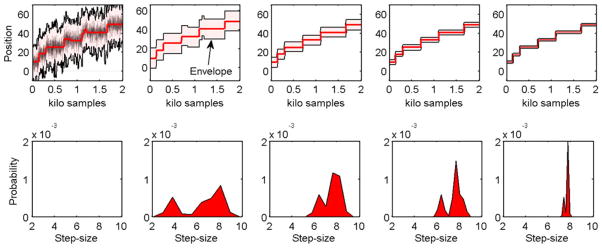
Iterations of step fits (left to right). Top row shows the step fits (red) and the envelope (shaded region) within which the fit was constrained. As iterations progress, the envelope is made narrower for better accuracy. Bottom row shows the smoothened step-size probability distribution obtained from the step size histogram of previous iterations fits. A Gaussian FIR filter is used for smoothening that reduces bias in the estimation of distribution. In the first iteration a constant weight on step sizes is used instead of a probability description hence it is shown blank. The smoothing level is reduced over iterations to get sharp histograms.

Fast and Slow Step Combinations

Whether the kinesin motor takes sub-steps is still being debated (see Block²). Coppin et al.³ suggested that kinesin takes a 3 nm step rapidly followed by another 5 nm step. Similarly, Nishiyama et al.¹⁷ suggested that kinesin takes two 4 nm steps in rapid succession. As the dwell time of the first step is small, it is especially challenging for current step detection methods to distinguish two 4 nm steps from a single 8 nm step. We asked whether our step-detection methodology can resolve such sub-steps. Figure 5 shows a simulation for a 3 + 5 nm step combination, where the dwell time of the 3 nm step is 0.6 ms (the data was sampled at 20 kHz). Over 80% of the 3 nm steps were correctly identified. The step size histogram converged closely to the true step sizes. In contrast, step-size histograms of the χ² method did not show a distinct bi-modal distribution, even when information about the total number of true steps was provided. Our algorithm shows a rapid decrease in the detection rate as the dwell time of the initial step is reduced, indicating that a minimum dwell time is required for reliable detection of substeps (see Table 1).

FIGURE 5.

Combination of fast 3 nm and slow 5 nm steps is generated (black trace) with noise of SD 2 nm (gray trace). Dwell time of the 3 nm step is chosen to be 0.6 ms. Dwell time of the slow step is random. From visual inspection the data appears to be composed of 8 nm steps only. However, our method (red trace) instead is able to correctly detect the 3 and 5 nm step sizes (inset). χ² method (blue trace), when provided with the information on the total number of true steps yields the histogram shown in blue (inset) which shows that our method significantly outperforms χ² method. When the total number of steps in not provided, the χ² method predominantly detects the 8 nm steps.

TABLE 1.

The table lists the minimum dwell times required for a fast step to be detectable by our method.

Noise	4 + 4	3 + 5
2	0.4 ms	0.6 ms
4	1.6 ms	3.8 ms
6	2.8 ms	9.2 ms
8	8.2 ms	20 ms

Step combinations are listed as fast + slow (4 + 4) and (3 + 5). Noise column is the white noise standard deviation added to the steps. These numbers are dependent on the sampling rate as well. The sampling rate for this set was 20 kHz. The numbers agree well to that predicted by the graph in Fig. 12.

Similar Step Sizes

A challenging problem in step detection is the resolution of steps of similar sizes. Since our algorithm is based on histogram iteration, similar sized steps may get diffused in the histogram smoothing process, leading to fusion of two or more step sizes into single averaged step size. To test the effect of smoothing, a simulation was performed with three step sizes, 3, 4 and 5 nm, occurring independently in the stepping signal. The three step sizes were easily resolved when using a noise level of 2 nm and sampling rate of 10 kHz (Fig. 6). χ²-method was not able to distinguish the three steps. At higher noise levels (>2 nm), the individual histogram peaks were either dislocated and/or additional spurious peaks appeared. In general, if the noise level is σ then our method can distinguish step sizes that differ by more than $\frac{\sigma }{2}$. However, this estimate also depends on sampling rate and dwell times as discussed below in the section ‘Trade-Off Between SNR and Dwell Time’.

FIGURE 6.

Stochastic stepping with mixed step sizes of 3, 4 and 5 nm is analyzed from data that has noise with SD 2 nm. Our method (red) is able to resolve these step sizes distinctly as evident in the step-size histogram. Insets show the progress of the algorithm iterations as the stepping probability is updated. Initial histogram is broad and steps sizes are not well resolved. However, in just a few iterations, distinct peaks appear and towards the end of the iterations, separated peaks are obtained. For the same data, χ² method’s estimates are spread out and incorrectly distributed.

Distributed Step Sizes

We next tested efficacy of our step detection methodology when there is no predominant step size that repeats or appears frequently in the data. In such a scenario, if the SNR is high, then most steps are identified and the distribution is reconstructed fairly well. If, however, SNR is low, then our algorithm will converge to multiple step sizes with gaps between them in the histogram (see Fig. 7a). Nonetheless, if the histograms are strongly smoothed before updating the penalty on steps, then the resulting histogram reflects a broader distribution (Fig. 7b). Therefore, our algorithm cannot predict whether underlying step-size distribution is continuous or discrete. However, if this information is available, then our algorithm can be suitably modified to improve its detection capability.

FIGURE 7.

Histogram comparison for distributed step size test. Stochastic stepping with average velocity of 500 nm/s and random step sizes was corrupted with noise of SD 5 nm and analyzed by our method. (a) Actual step size distribution (black trace) is broad with peaks at 4 and 8 nm. Our method (red trace) concentrates most of the steps at the 4 and 8 nm due to its preferential treatment to higher probability steps. (b) In this case, our method was modified to artificially smoothen the histogram for computation of step-size probability. The parameter ‘smooth’ in the figure refers the to the spread of the Gaussian filter applied to the histogram. The resulting step-size histogram reflects this as reproducing the distributed nature of the step sizes.

Dynamics Compensation

The efficacy and limitations of our step detection methodology in addressing probe-dynamics was assessed for three cases. In the first case, a train of noisy 5 nm steps is filtered by the slow dynamics of the probe using cutoff frequency of 20 Hz. The steps are hard to discern (gray trace in Fig. 8a) by eye. In addition, χ² method clearly fails to identify correct step size and location even when the information on the true number of steps is made available. In contrast, our method uses knowledge about probe dynamics to compensate for the dynamics and reveal the stepping signal (Fig. 8a).

FIGURE 8.

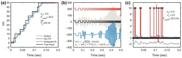
Dynamics compensation feature tested in simulations for different scenarios. (a) Stepping train of 5 nm is generated with stochastic dwell times. Noise of σ = 3 nm is added to the step signal and passed through a low pass filter with cutoff at 20 Hz. The filtered noisy signal is analyzed by our method (red trace) and the χ² method (blue trace). Our method is able to underlying step signal with good accuracy and the histogram (inset) shows most steps were 5 nm except some steps (that had small dwell times) were identified as 4 nm instead. On the other hand, χ² method fits steps disregarding dynamics effects hence all the identified steps are spurious. (b) A second order dynamics effect is tested. Square signal is passed through a filter that amplifies certain frequencies and therefore we observe amplified oscillations and overshoots for square steps (it is not due to noise). The input signal has moderate amount of noise, SD = 4. Under these conditions as well, our algorithm finds steps correctly with histogram (inset) of step sizes matching the true one. χ² method instead shows a variable step size as different stepping frequencies have different amplification dictated by the dynamical model. (c) Spikes in the data are also detected by our method under moderate noise assumptions. Impulses generated by a rising step rapidly followed by a falling step are filtered via first order dynamics. From the resulting trace (gray), it is difficult to make out all the steps and their magnitudes. Our method does much better job of detecting step location and their magnitudes (see histogram in inset). χ² method instead tries to fit steps to the observed data and fails to identify the impulsive inputs.

In a second test case, a square wave input is generated with decreasing dwell time. Noise is added to this signal and then passed through a second order filter, which has a clear resonance. Our method is able find the hidden steps with a good estimation of the step sizes that generated the observed data. The χ² method fails to do so (Fig. 8b).

In the third case, we evaluated the capability of detecting spikes or impulses, a combination of a rising step quickly followed by a falling step of the same size. Noise was added to such spikes and passed through a first order filter. The resulting signal looks highly distorted (gray trace in Fig. 8c). Our method handles such data without any modification if provided with the correct filter model. This kind of data is much more difficult to analyze and noise has severe adverse effects compared to other stepping signals. χ² method gives no indication of spikes in the data.

Non Stepping Data

An important aspect of step detection is to discern the difference between stepping and non-stepping data. When presented with a smoothly varying signal with added noise, our method tries to fit minimum number of small steps, such that the χ² error is nearly the same as the true variance. As discussed in a later section, beyond a limit, small step sizes and fast arrival rates are not handled well by our algorithm and it tends to fit steps that are not actually present as in Fig. 9a. Similarly, other algorithms also fail to accurately detect the steps. However, we propose a method to evaluate the quality of fit in terms of confidence that underlying data has steps.

FIGURE 9.

Plots here compare the average LLR for different types of data. LLR compares the likelihood of the observed data being originated from stepping action against a smoothly varying motion. (a) Data (gray) is originating from a smooth signal (black). Our algorithm fits a step signal to it with distinct steps. By connecting the plateaus of the steps, a smooth signal is generated (green). This smooth signal closely matches the true smooth signal (see inset). By comparing the χ² error for the smooth signal (green) against that of the step fit (red), LLR can be obtained. Smaller LLR indicates that a smooth signal may fit the data as well as a stepping signal. (b) Underlying the data is a stepping signal but not evident by looking at the data. An LLR of 0.09 indicates the underlying data is better explained by stepping signal rather than a smooth signal. (c) Steps are evident from the data itself. The corresponding LLR is also huge which is a confident measure of underlying signal being a stepping signal.

Evaluation with Experimental Data

We used a bead-motility assay to collect experimental data on kinesin steps obtained under a constant load provided by optical tweezers. The sample preparation is similar to that described in Hancock and Howard⁸ and is discussed briefly in the ‘Methods’ section. The experimental setup is similar to Lang et al.¹³ and instrument calibration was done as described in Aggarwal and Salapaka.¹ There is drift in the data and extrinsic disturbances also introduce significant non-Gaussian noise. In this regard, the experimental data provide a good test of the robustness of our method under non-ideal conditions. We compared the fit of the steps to the experimental data using the χ² method, as well as our new method. It was determined that the cargo was carried by a single kinesin molecule and thus it is expected that the cargo steps by approximately 8 nm (see supplementary note) with deviations expected due to experimental uncertainties. The χ² method detects step sizes that are broadly and unsymmetrically distributed about 7.5 nm spanning 6–10 nm range (Fig. 10b), whereas our method results in a predominant peak near 7.5 nm (see Fig. 10a). These results are consistent with 8 nm step-size assumption. Other peaks arise possibly due to drift and disturbance effects on the bead. Some negative steps near 7.5 nm were also observed and may be attributed to kinesin slippage under load.¹¹

FIGURE 10.

Fitting on experimental data obtained from kinesin-bead assay. (a) Histogram of the step sizes obtained by using our method. (b) Histogram of step sizes obtained by using chisquare method (number of steps was constrained to be equal to that obtained by our method). (c) Experimental power spectrum (gray) was obtained from a portion of data that did not contain any steps on visual inspection. This was fitted with simulated power spectrum of filtered noise (red) for a thermal noise level of 15 nm, measurement noise of 1.5 nm and cutoff frequency of 600 Hz. The dynamical model obtained from this fit was provided to our algorithm for fitting. The fit is not good representing deviations from assumed Gaussian noise statistics. Expected cut-off frequency for a stretched kinesin linkage is much higher but due to large extrinsic noise. Therefore, a conservative model (simulated power spectrum should be above experimental spectrum) is a better choice to avoid fitting spurious steps. (d) Step fits, using our method (red) and chisquare method (blue) on experimental data (gray). Fits look similar but histograms differ considerably. Our method gives a strong peak around 7.5 nm in contrast to a broad distribution given by chisquare method. Deviations from expected 8 nm step size is attributed to experimental uncertainties, and external noise sources including drift and vibrations and electrical line noise that do not fit well to assumed Gaussian statistics.

In addition to optical tweezer data, we collected AFM experimental data on the unfolding behavior of the muscle protein, titin this data was particularly useful to validate the step detection method and its ability to compensate for probe-dynamics. The 27th immunoglobulin-like module of cardiac titin has 8, nearly identical, domains that unfold when a force is applied.⁷ In a typical AFM experiment, the molecule’s ends are attached between AFM cantilever tip and the substrate that sits on a piezo actuated positioning system. The separation between the substrate and the cantilever tip is controlled to maintain a constant tension in the molecule. When the protein unfolds, it relaxes quickly and the instrument responds by pulling the molecule to maintain a constant force. However, the response of the system to the unfolding event takes a certain time to settle and consequently the transition of the cantilever state that results from a protein conformation change is smooth, unlike the sharp unfolding event itself. If the unfolding events occur rapidly then, the protein configuration changes while the system is reaching its new equilibrium position, determined by the effects of the previous unfolding event of the protein. This is indeed the case with our experimental data shown in Fig. 11. We hypothesized a simple first order model for the system behavior in response to an unfolding event. The model was estimated offline using only one step response (see ‘Methods’ section) and was used to correct for the smoothing process introduced by the dynamics. An estimate of 24 nm for the unfolded protein module length was obtained as shown in the histogram of Fig. 11. The χ² method finds fewer 24 nm steps, corresponding to those steps that have large dwell times. Currently, researchers discard experimental data, that is distorted due to probe dynamics which current methods cannot incorporate. With our method, such data can now be retained and analyzed. Consequentially, the range of loads under which protein folding and unfolding is investigated can be increased. This is because under increased loads, domains unravel faster whereby the effect of an unfolding event can overlap with another unfolding event. With our step detection methodology, steps can be recovered from such data.

FIGURE 11.

Dynamics compensation feature of our method for titin pulling experiment. The titin pulling experiment using AFM results in data that has steps but sharp transitions are smoothed due to limited response time of instrumentation and/or the sample itself. The response time was estimated from the data itself by inspecting one of the steps that has large dwell time. This response time was provided to the algorithm for fitting and noise was also estimated from the stationary portion of the data. The resulting fit is relatively accurate finds steps of 25–25 nm. A small step (in the initial portion of the data) is experimental artifact of AFM engaging with the sample. In contrast, χ² method only identifies steps that have large dwell time. Location of identified steps is clearly erroneous and fast steps are incorrectly estimated in its size as well. As a result, multiple step sizes are estimated instead of a uniform 24 nm steps.

Limitations

Distinguishing Between Stepping and Non-Stepping Data

To determine whether observed data contains discrete steps or reflects a continuous trajectory is particularly challenging when steps occur at a fast pace and step-sizes are small with respect to the standard deviation of the noise. Under these condition, step-detection methods, including our own will show steps even when there might be no steps in the true signal.

Here we provide a measure to guard against the false interpretation of steps. We compare the fit by discrete steps (denoted by x̂) to a fit by a smooth signal (denoted by x̃). The smooth signal, x̃, is generated from x̂ by joining the mid-points of two subsequent step-plateaus thereby resulting in smoothing of discrete stepping signal. Simulations show that if the underlying signal is smooth, then the smooth fit to the data, determined from the estimate produced by the step-detection methodology will provide a good match to the true smooth signal (Fig. 9a).

To further determine the quality of a step fit with respect to a smooth fit, we compute the ratio of probability for a step fit x̂ over that for a smooth fit x̃. The larger the logarithm of the ratio (called log-likelihood ratio (LLR)), the greater the confidence that the stepping is accurate reflection of true signal. Conversely, a negative or small LLR indicates that the data is equally likely to result from a smooth continuous trajectory. LLR is defined as follows

$$\begin{array}{l}\frac{P(\widehat{x})}{P(\stackrel{\sim }{x})}=\frac{{\prod }_{k=1}^N\frac{1}{\sqrt{2\pi }{\sigma }^2}{e}^{-\frac{{(y_k-{\widehat{x}}_k)}^2}{2{\sigma }^2}}}{{\prod }_{k=1}^N\frac{1}{\sqrt{2\pi }{\sigma }^2}{e}^{-\frac{{(y_k-{\stackrel{\sim }{x}}_k)}^2}{2{\sigma }^2}}};\\ logP(x)-logP(\stackrel{\sim }{x})\\ =\frac{1}{2{\sigma }^2}\left[\sum _{k=1}^N{(y_k-{\stackrel{\sim }{x}}_k)}^2-\sum _{k=1}^N{(y_k-x_k)}^2\right]\\ \mathit{LLR}:=\frac{1}{N}[logP(x)-logP(\stackrel{\sim }{x})]\end{array}$$

where P(x̂) is the probability of step-fit, x. P(x̃) is the probability of the smooth fit, x̃. LLR greater than 0.08 should typically indicate a stepping behavior and LLR less than 0.05 is likely to mean the fit is not reliable and underlying fit could be smooth. Figure 9 compares the LLR of a fit for a smooth signal vs. a stepping signal for different scenarios.

Trade-Off Between SNR and Dwell Time

There is general agreement that the ability to detect steps depends on the signal-to-noise ratio (SNR), that is the ratio of step-size to the standard deviation of the noise. When the SNR is small, steps are harder to detect with accuracy. Another, less referenced factor in resolving steps is how the dwell-times, or equivalently the number of samples obtained for a step, will affect the detection capability. Consider, for example, a stepping signal, x, where there is single step of size m in the middle of data that has N samples. Given that y_k = x_k + n_k where noise n_k has zero mean with a standard deviation σ, then the SNR is $\frac{m}{\sigma }$. Also, as discussed earlier, the cost J(x) of the true signal x is such that J(x) ≈ Nσ² + W, assuming a constant penalty for every step irrespective of step-size. Let us consider an estimate x̂ that has no steps with a constant value equal to the mean of the data given by $\frac{m}{2}$. If we assume that W = 9σ², then we have $J(\widehat{x})={\sum }_k{(y_k-{\widehat{x}}_k)}^2\approx N{\sigma }^2+N\frac{m^2}{4}$. We would like the true signal to have the smallest cost and therefore we desire $J(\widehat{x})-J(x)=N{\sigma }^2+N\frac{m^2}{4}-N{\sigma }^2-W=N\frac{m^2}{4}-9{\sigma }^2>0$. Thus we would like $N>36{(\frac{\sigma }{m})}^2=36\frac{1}{SN{R}^2}$. This relationship, although illustrated on an instance of an estimate x̂, holds qualitatively in general. Thus the number of samples required between steps, for good performance of our step-detection methodology has to be greater than 1/SNR².

The quantitative relationship between the SNR, dwell-time and detection capability for step-detection methodologies is typically not assessed in the literature. Here, we provide such an analysis. We perform step detection using a square wave signal that has gradually decreasing dwell time (gray trace in Fig. 12a). It is similar to a sinusoidal frequency sweep, except the sine wave is replaced by a square wave. Several such simulations are performed for a given noise level and the resulting step fits are averaged (red trace in Fig. 12a). We observe that for longer dwell times (low frequency data) the averaged step-fits look like the original square waves as expected However, for shorter dwell times, the square wave amplitude of the averaged fit is reduced. This happens because, on an average, steps with shorter dwell times were missed. The dwell time beyond which the local amplitude curve drops (cutoff frequency, Fig. 12a) below a chosen threshold (85% of amplitude), the minimum dwell time required to detect a step can be determined. The corresponding SNR is the peak-to-peak amplitude of the original square wave divided by the known noise standard deviation. Hence the dwell-time and SNR pair is obtained for different noise levels and a graph is plotted (Fig. 12b). Given one of the quantities, the limit on the other can be predicted from the graph.

FIGURE 12.

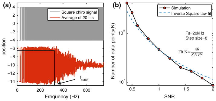
(a) Top trace (black) is a square chirp, a square wave with linearly decreasing dwell time. Bottom trace (red) is an average of 20 fits, obtained by running our algorithm on square chirp signal with noise added. The algorithm is able to detect steps with larger dwell time (low frequency square wave) in every simulation thus average fit has full amplitude, but steps with smaller dwell time (high frequency steps) are often missed out and therefore the average of the fits has diminished amplitude. By observing frequency after which amplitude drops below a threshold (here the original amplitude is 8 nm and cutoff threshold is chosen to be 7 nm), we can estimate the stepping frequency beyond which a fit is unreliable. The abscissa lists the frequency of the square wave. One square wave has two steps therefore the stepping frequency is twice the number obtained from this graph. By normalizing the sampling frequency (samples/s) with stepping frequency (steps/s) we can obtain the required number of samples per step. This number is plotted against SNR in (b). (b) Black solid line is the number of samples points required to detect steps in reliable manner for a given SNR. An inverse square law relationship is observed, evident from the fit (blue dashed line). The constant of proportionality (46) reflects the penalty on the steps. Bigger number would mean larger penalty. This graph can be used to predict whether a step of a given size and dwell time will be detectable under a given SNR in a reliable manner. For example, for a sampling rate of 10 kHz, we wish to know the minimum dwell time of a 2 nm step will be detectable when the noise is also 2 nm. This corresponds to SNR = 1. From the graph, approximately 45 samples per step will be required. This corresponds to a dwell time of $\frac{45}{{10}^4\text{Hz}}=4.5\text{ms}$.

Computational Costs

The straightforward implementation of our method can be computationally expensive. This reflects the large search space required for the many possible step functions and the need to compare their respective costs (J(x̂)). In the dynamic programming approach, candidate step functions are constrained to take values along closely spaced grid lines. Candidate step functions are also allowed to take steps at any sample point. The computational complexity has exponential dependence on the number of grid levels, M and number of sample points, N. Then the total number of computations can be estimated to be M^N. For example, if 1 s of data ranges from 0 to 1000 nm and is sampled at 10 kHz, then a grid resolution of 1 nm corresponds to N = 10⁴, M = 10³. Therefore, the number of computations required is 10³⁰⁰⁰⁰. This is a huge number. Dynamic programming technique can reduce the computational complexity to NM². For the example above, this computes to 10¹⁰ which is tractable. However, many of the computations are unnecessary because true signal is expected to interpolate the noisy data which span a small number of grid points. By eliminated computations for grid points that are unlikely to be a part of the step-fit, we can significantly reduce the computational complexity further. For example, if the noise level (σ) in the data is 5 nm, then one can expect that grid points lying beyond 3σ of the local mean of the data will not be a part of the step-fit. Therefore, we can bound the data in an envelope of width approximately 6σ = 30 nm, within which we search for an optimal fit. In this case, M = 30 and the total number of computations is of the order of 10⁷. However, during our iterations, we start with crude fineness to the data space such that M = 50. In subsequent iterations, the fineness is increased by reducing the envelope width but keeping the same M. This allows for better accuracy without taxing computations. Another level of efficiency is achieved because the computations can be parallelized without a loss in performance. Therefore, the methodology can take advantage of multi-core processors and the parallel computation features of MATLAB. Our implementation is on a quad-core computer (2.5 GHz), this brings additional speed acceleration by 4 times. Table 2 shows computation time required for different sample lengths. Given our code optimization, the implementation of our method runs fast, in fact much faster than the simple implementation of χ²-method (for larger data sets, N>10⁴).

TABLE 2.

Mean computation time (in seconds) variation with data length.

Sample length	103	5 × 103	104	5 × 104	105	5 × 105
Our method	2	9	17	32	54	242
χ2-method	0.6	6	7	30	60	305

Sampling rate = 10 kHz. Noise σ = 5 nm. V_avg = 500 nm/s. Number of iterations = 8. Final grid resolution less than 0.2 nm. The nonlinear relation between sample length and computation time is likely due to the parallelization of the code into four cores. Our implementation of χ²-method is much faster than provided by the original authors of the method, and also parallelized. The reported times are for our implementation of optimized χ² method. We observe that scaling of computational complexity of our method with number of samples is slower than that of χ²-method. Times scales being comparable for the two methods indicates our method can be utilized for practical datasets.

A METRIC ON PERFORMANCE

Quantities that are commonly employed to evaluate detection methods are true positive rate (TPR) and false positive rate (FPR). TPR is the percentage of true steps that are correctly identified by the algorithm. FPR is the percentage of false steps that are identified by the algorithm and are not actually present in the data. The computation of these metrics is discussed in the ‘Methods’ section. None of these quantifiers, by themselves, is a good measure of the performance of the algorithm. Thus, a more comprehensive measure is needed. The Receiver Operator Characteristic (ROC)⁵ provides a reasonable means to compare different methods. For a given algorithm, the FPR and TPR values can be determined and the coordinates (FPR, TPR) placed on a graph of TPR vs. FPR with the axis limits for both FPR and TP between 0 and 100. The directed distance of the (FPR, TPR) point from the diagonal line joining the point (0,0) to the point (100,100) provides a good measure of the method’s performance. The measure (the ROC measure) is positive if it lies above the diagonal line. The largest positive distance from the line is the point (0,100) which corresponds to FPR = 0 and TPR = 100. Also for a fixed FPR value, the higher the TPR value the better the measure will be. Similarly, for a fixed TPR value, the lower the FPR value, the higher is the value of the measure (the distance from the diagonal line will be higher). Thus this measure has most of the characteristics desired for a quantifier. A single performance measure, a metric defined using ROC was employed for this purpose. Each data point was generated by simulating approximately 100, 8 nm steps with an average velocity of 500 nm/s (for comparison purpose, no filters are applied to simulate probe dynamics). Various noise levels were added to the input ranging from a standard deviation of 1–8 nm with a sampling rate of 2 kHz. The performance measure was compared for different step detection methods for different output noise levels as shown in Fig. 13. The ROC analysis reveals several interesting properties. (1) Performance for all methods is reduced with increasing noise, however our method is least affected. (2) The ROC plot has low variance which means it provides consistent results over various simulations, providing better reliability. (3) This metric effectively compares and quantifies performance of other methods as well. We find that the χ²-method is the next best after our method, followed by the t-test and dGWT method. The VT method offered the lowest performance in our comparisons.

FIGURE 13.

Comparison of ROC performance metric for different methods under various noise levels. Performance was computed by evaluating the average TPR (percentage of correctly found steps) and FPR (percentage of spurious steps) for 50 simulations of stochastic stepping consisting approximately 100 steps with white noise added to the stepping signal. The TPR and FPR was then fused into a single ROC performance number. Under this performance metric, our method is better than existing methods for all tested noise levels and the drop in performance with increasing noise is least for our method. Other parameters for the simulations are included in the plot. The error bars mark the maximum and minimum values of the performance number obtained over the 50 simulations. There is a sudden drop in performance of our method at around 6 nm noise variance for our method which is consistent with our analysis on limits of detection that predicts sudden drop in performance for noise SD of 6.5. However, it still performs better that other methods. The performance number of other methods plotted here is for optimized parameters using the knowledge of true signal, therefore represents an upper bound on their performance.

Methods were compared using the optimal settings for the respective parameters. The settings were computed based on the information about the actual number of steps in the simulations. Therefore the performance graph of other methods in Fig. 13 represents an upper bound on their actual performance. In contrast, our method operates in a parameter free manner, incorporating noise statistics, which was estimated automatically.

DISCUSSION

The advent of new instrumentation is driving a rapid expansion of single molecule studies. There is an urgent need for methods to better decipher single molecule data and resolve molecular events and behavior. This single molecule data frequently contains stepping characteristics, but noise and filter dynamics can obscure the steps. An automated method not only relieves the burden of manually picking out steps but also eliminates the bias introduced by manual detection. Advances in signal processing techniques have led to improved analytical capabilities that can be leveraged for a better treatment of experimental data from biological studies.

We have developed a novel step detection methodology that fits data while penalizing steps in an optimization framework with an iterative strategy for adjusting the penalty based on the histogram of step sizes. In the proposed method, a step fit is performed by optimizing a cost function composed of the χ² error and a penalty on total number of steps in the fit. The histogram of step sizes for the fit is used to reweight the penalty on the number of steps and the process is repeated in an iterative manner until step-size histograms do not change over iterations. In essence, it searches entire data set for a pattern of frequently occurring steps and then optimally place such steps in the appropriate locations. We have demonstrated that our methodology has several advantages over existing step detection methods: (1) It produces sharp step-size histograms when the underlying data has a unimodal step size distribution. This helps in quantifying the number of steps of a particular size. (2) It has the ability to compensate for probe dynamics if a suitable model of the dynamics is available. Probe dynamics distort step signals into smoothly varying signals and obscure the steps. Existing step detection methods fail to identify the underlying steps, but our method corrects for the smoothing that results from probe dynamics and reveals the hidden step signal. (3) Unlike other methods, our algorithm also functions without specifying any parameters. Noise statistics is a required input, but can be automatically estimated from the experimental data. However, a model for sensor dynamics is required if compensation is desired. (4) In comparison with other methods, it has the highest accuracy in terms of detection of true steps and not producing false steps. (5) It can also detect events characterized by impulsive/spiking behavior. (6) The flexibility offered by having an optimization framework and an intuitive cost function can be utilized in a variety of ways. For example, estimation of parameters, compensation of nonlinearities and integrating existing knowledge about the system into the methodology.

We also developed a strategy to quantify the limitations of our step-detection method, as well as to compare the limitations of other step detection methods. An undesirable artifact of our method is that it will fit steps regardless of whether the underlying signal has steps or varies smoothly; most step detection methods suffer from this drawback. Nonetheless, we provide a quantitative means to judge the quality of the fits by computing the likelihood of the fit being produced from stepping data versus smoothly varying data. Another apparent limitation of the method is its computational complexity. The core of the algorithm can be implemented easily. We have implemented complexity reduction techniques that render fast execution of the algorithm. The code for the algorithm implemented on MATLAB can be downloaded from the website, http://nanodynamics.ece.umn.edu. The code can further utilize the parallel processing capability of MATLAB with multiple-core computers if available.

We provide in-depth analysis of the effect of various properties of a stepping data, like dwell-times and noise levels, that affect the performance of step detection methods. The SNR and dwell-time trade-off analysis shows that higher dwell-times are required to detect steps when SNR reduces. An inverse square-law relation between dwell-time and SNR was observed. We further provide quantitative means to characterize these effects for validation and comparison. A new measure for comparison (ROC) was introduced that effectively quantifies the performance of a step detection algorithm based on its detection accuracy and ability to discard spurious steps. We analyzed the relation between SNR and stepping rate that needs to be satisfied to ensure that our step-fitting method can be relied upon. We have tested the algorithm for various scenarios of stepping data and demonstrated its effectiveness over other methods in a comprehensive manner. The method was also tested on experimental data obtained from optical tweezers and AFM studies.

With this step-detection method we have introduced a new means of determining steps in single molecule data, that outperforms existing methods. Our method yields higher TP, lower false positives, for shorter dwell-times and lower SNR. Our methodology also uniquely address the smoothing effect of probe-dynamics to increase step-detection performance and applicability. These capabilities should enable the exploration of single molecule behavior at higher temporal and spatial resolutions.

METHODS

Kinesin Purification and Bead Motility Assay

The purification of recombinant kinesin and the kinesin-bead motility assay were based on previously reported methods with only minor modifications.⁸ Briefly, the coexpression plasmid DmKHC encodes the full length Drosophila kinesin 1 heavy chain and was a gift from William Hancock. The plasmid was transfected into E. coli strain BL21(DE3) (Novagen, Inc.) and protein expression was induced by isopropyl Beta-p-thiogalatopyranoside. Bacteria were pelleted by centrifugation for at 6000g, and were then resuspended in lysis buffer (50 mM sodium phosphate, 300 mM NaCl, 40 mM imidazole, 5 mM β-mercaptoethanol, 10% glycerol, pH 8.0), frozen in liquid nitrogen, and then stored at −80 °C. The his-tagged kinesin was purified from clarified bacterial lysate on a Ni-nitrilotriacetic acid (NTA) agarose column (QIAGEN, Inc., Santa Clarita, CA). Column buffers contained the following: 50 mM sodium phosphate, 300 mM NaCl, 1 mM MgCl₂, 100 μM MgATP, 5 mM β-mercaptoethanol (added just before using), and either 60 mM (wash buffer) or 500 mM (elution buffer) imidazole, pH 7.0. Subsequently, the DmKhc motor was further purified by microtubule affinity^15,26 DmKhc was incubated with taxol-polymerized tubulin in the presence of 2 mM AMP-PNP for 30 min. The assembled microtubules with bound kinesin were copelleted through a 15% sucrose gradient. The pellet was resuspended and kinesin was eluted in buffer containing taxol and 10 mM ATP. The microtubules were pelleted and the supernatant containing purified kinesin was brought to 20% sucrose, aliquoted and flash frozen.

Labeled microtubules were prepared by mixing 50 μL of 20 μg/mL tubulin and 1 μL of 4 μg/mL rhodamine-labeled tubulin (T240A and TL331M from Cytoskeleon Inc.) in MTB [MTB = (1 mM GTP, 1 mM DTT, 10 μM taxol in BRB80)] at 37 °C for 20 min. Free tubulin was separated from microtubules by layering the microtubule solution over cushion buffer (60% glycerol, 40% BRB80, 1 mM GTP, 1 mM DTT, 10 μM taxol; BRB80 = (80 mM PIPES, 1 mM EGTA, 1 mM MgCl₂, pH 6.9)) followed by centrifugation at 27,000g for 35 min. The supernatant was discarded and the pelleted microtubules were resuspended in 50 μl MTB. Final working solution contained 1:100 dilution of the stock in MTB. Beads (Polysciences, 0.5 μm diameter, 2.68 % solids, carboxylate YG) were incubated in BRB80 and 5 mg/mL casein (Sigma C4765)in for 1 h in a bath sonicator. These beads were incubated with diluted kinesin-1 on ice for 1 h in BRB80CA (10 μM ATP in BRB80). The bead-kinesin stoichiometry was adjusted so that a small percentage (less than 30%) of the beads tested on optical tweezers were motile. Sample was prepared by creating a fluid chamber formed by coverslips separated and held together by double sided tape. The coverslip that is in proximity to microscope objective was precoated with poly-L-lysine. Microtubule solution is introduced in the chamber and incubated for 5 min to allow microtubules to adhere to the poly-L-lysine treat 132; tubules to adhere to the poly-L-lysine treat-clear unbound microtubules. Following this, blocking buffer (2 mg/mL BSA in MTB) was introduced in the chamber and incubated two times for 10 min each.

Finally, beads with bound kinesin motor protein was diluted into motility buffer (100 μM ATP, 0.45 mg/mL glucose, 200 μg/mL glucose oxidase, 35 μg/mL catalase, 0.5% 2-mercaptoethanol in MTB) and introduced in the fluid chamber. The sample was observed on an inverted optical tweezers microscope setup. A freely diffusing bead is trapped, calibrated and then a piezo stage is used to bring a microtubule (visible under fluorescence) in close proximity to the trapped bead. If motility is observed in bead position then data is logged for either stall force or constant force study.

AFM Experiment

A sample of solution of the engineered octamer of I27 (the 27th Immunoglobulin-like module of cardiac titin) was deposited for 20 min on the surface of a freshly exposed template stripped gold.⁹ This is then placed inside a AFM liquid cell and the surface was rinsed with Phosphate Buffered Saline (the same buffer of the specimen). After optical realignment and thermal equilibration of the system, force-clamp AFM experiments were performed applying on the protein a pulling force of 110 pN. The details of the instrumentation are reported by Materassi et al.¹⁴ The dynamics in the titin stretching experiment was assumed to be governed by the ordinary differential equation given by τẏ+ y = x, where x is a staircase function representing the length of the polymer in its current (partially) unfolded state at equilibrium, y is the measured extension of the piezoelectric actuator plus the cantilever deflection and τ is a time constant fitted to match the last step in the curve (that is usually an isolated unfolding event). τ was determined by giving a step input to the system and recording the time that it took for the system to reach 63% of the commanded step input.

Performance Measure Computation

A step in the estimated signal is declared TP if it is in the neighborhood of an actual step (defined as a window size of 10 samples on either side of the actual step) and the step height is within a tolerance (± 2 nm) of actual step height. If there are multiple such steps, the one closest to the actual step is selected to represent a true step and others are discarded. Also, the declared true step is not allowed to represent any other step in the actual signal. This way there is a unique step in the actual signal for each TP step. All the identified steps that are not true positives are declared false positives, FP. Likewise, actual steps that are not represented by any TP step become unidentified steps or false negatives (FNs). These numbers can be expressed as a percentage of the total number of actual steps (N₀). Therefore we get the TPR, $\mathit{TPR}=100\frac{TP}{N_0}$, and the FPR, $\mathit{FPR}=100\frac{FP}{N_0}$. For a given method, these numbers vary with the amount of noise in the system, frequency of arrival of steps. Step functions with staircase profile were generated with a Poisson distributed dwell times with a specified mean (500 nm/s with sampling rate of 2 kHz). Step size was also fixed (8 nm) but not known to any of the detection methods. For a given noise level, 50 simulations were performed and analyzed by various detection methods. The TPR and FPR was computed for each simulation. TPR and FPR is used to compute performance measure given by $\rho =\frac{1}{70.7}sin\left({tan}^{-1}\left(\frac{\mathit{TPR}}{\mathit{FPR}}\right)-\frac{\pi }{4}\right)\sqrt{{\mathit{TPR}}^2+{\mathit{FPR}}^2}$. It is essentially the distance of the point (FPR,TPR) from the line that is at 45° to the horizontal axis of TPR vs. FPR plot normalized by the maximum distance of 70.7. This is the distance of the point (0,100) from the 45° line. This line is also called line of no distinction because any point on this line represents equal probability of an identified step being true or spurious. Mean ρ is plotted in Fig. 13 with error bars indicating the maximum and the minimum values obtained over the 50 simulations.

References

- 1.Aggarwal T, Salapaka M. Real-time nonlinear correction of back-focal-plane detection in optical tweezers. Rev Sci Instrum. 2010;81(12):123105–123105-5. doi: 10.1063/1.3520463. [DOI] [PubMed] [Google Scholar]
- 2.Block S. Kinesin motor mechanics: binding, stepping, tracking, gating, and limping. Biophys J. 2007;92(9):2986–2995. doi: 10.1529/biophysj.106.100677. [DOI] [PMC free article] [PubMed] [Google Scholar]
- 3.Coppin C, Finer J, Spudich J, Vale R. Detection of sub-8-nm movements of kinesin by high-resolution optical-trap microscopy. Proc Natl Acad Sci USA. 1996;93(5):1913–1917. doi: 10.1073/pnas.93.5.1913. [DOI] [PMC free article] [PubMed] [Google Scholar]
- 4.Cornish P, Ha T. A survey of single-molecule techniques in chemical biology. ACS Chem Biol. 2007;2(1):53–61. doi: 10.1021/cb600342a. [DOI] [PubMed] [Google Scholar]
- 5.Egan J. Signal detection theory and ROC-analysis. New York: Academic Press; 1975. [Google Scholar]
- 6.Engel A, Müller D. Observing single biomolecules at work with the atomic force microscope. Nat Struct Mol Biol. 2000;7(9):715–718. doi: 10.1038/78929. [DOI] [PubMed] [Google Scholar]
- 7.Fernandez J, Li H. Force-clamp spectroscopy monitors the folding trajectory of a single protein. Science. 2004;303(5664):1674–1678. doi: 10.1126/science.1092497. [DOI] [PubMed] [Google Scholar]
- 8.Hancock W, Howard J. Processivity of the motor protein kinesin requires two heads. J Cell Biol. 1998;140(6):1395–1405. doi: 10.1083/jcb.140.6.1395. [DOI] [PMC free article] [PubMed] [Google Scholar]
- 9.Hegner M, Wagner P, Semenza G. Ultralarge atomically flat template-stripped Au surfaces for scanning probe microscopy. Surf Sci. 1993;291(1–2):39–46. [Google Scholar]
- 10.Hirokawa N, Noda Y, Tanaka Y, Niwa S. Kinesin superfamily motor proteins and intracellular transport. Nat Rev Mol Cell Biol. 2009;10(10):682–696. doi: 10.1038/nrm2774. [DOI] [PubMed] [Google Scholar]
- 11.Hyeon C, Klumpp S, Onuchic J. Kinesin’s backsteps under mechanical load. Phys Chem Chem Phys. 2009;11(24):4899–4910. doi: 10.1039/b903536b. [DOI] [PubMed] [Google Scholar]
- 12.Kubelka J, Hofrichter J, Eaton W. The protein folding ‘speed limit’. Curr Opin Struct Biol. 2004;14(1):76–88. doi: 10.1016/j.sbi.2004.01.013. [DOI] [PubMed] [Google Scholar]
- 13.Lang M, Asbury C, Shaevitz J, Block S. An automated two-dimensional optical force clamp for single molecule studies. Biophys J. 2002;83(1):491–501. doi: 10.1016/S0006-3495(02)75185-0. [DOI] [PMC free article] [PubMed] [Google Scholar]
- 14.Materassi D, Baschieri P, Tiribilli B, Zuccheri G, Samorì B. An open source/real-time atomic force microscope architecture to perform customizable force spectroscopy experiments. Rev Sci Instrum. 2009;80:084301. doi: 10.1063/1.3194046. [DOI] [PubMed] [Google Scholar]
- 15.McGrail M, Gepner J, Silvanovich A, Ludmann S, Serr M, Hays T. Regulation of cytoplasmic dynein function in vivo by the Drosophila Glued complex. J Cell Biol. 1995;131(2):411–425. doi: 10.1083/jcb.131.2.411. [DOI] [PMC free article] [PubMed] [Google Scholar]
- 16.Moffitt J, Chemla Y, Smith S, Bustamante C. Recent advances in optical tweezers. Biochemistry. 2008;77(1):205–228. doi: 10.1146/annurev.biochem.77.043007.090225. [DOI] [PubMed] [Google Scholar]
- 17.Nishiyama M, Muto E, Inoue Y, Yanagida T, Higuchi H. Substeps within the 8-nm step of the ATPase cycle of single kinesin molecules. Nat Cell Biol. 2001;3(4):425–428. doi: 10.1038/35070116. [DOI] [PubMed] [Google Scholar]
- 18.Oberhauser A, Hansma P, Carrion-Vazquez M, Fernandez J. Stepwise unfolding of titin under force-clamp atomic force microscopy. Proc Natl Acad Sci USA. 2001;98(2):468–472. doi: 10.1073/pnas.021321798. [DOI] [PMC free article] [PubMed] [Google Scholar]
- 19.Rief M, Rock R, Mehta A, Mooseker M, Cheney R, Spudich J. Myosin-V stepping kinetics: a molecular model for processivity. Proc Natl Acad Sci USA. 2000;97(17):9482–9486. doi: 10.1073/pnas.97.17.9482. [DOI] [PMC free article] [PubMed] [Google Scholar]
- 20.Sakamoto T, Amitani I, Yokota E, Ando T. Direct observation of processive movement by individual myosin V molecules. Biochem Biophys Res Commun. 2000;272(2):586–590. doi: 10.1006/bbrc.2000.2819. [DOI] [PubMed] [Google Scholar]
- 21.Sakmann B. Elementary steps in synaptic transmission revealed by currents through single ion channels. Biosci Rep. 1992;12(4):237–262. doi: 10.1007/BF01122797. [DOI] [PubMed] [Google Scholar]
- 22.Schneidman E, Freedman B, Segev I. Ion channel stochasticity may be critical in determining the reliability and precision of spike timing. Neural Comput. 1998;10(7):1679–1703. doi: 10.1162/089976698300017089. [DOI] [PubMed] [Google Scholar]
- 23.Sehgal H, Aggarwal T, Salapaka M. High bandwidth force estimation for optical tweezers. Appl Phys Lett. 2009;94(15):153114. [Google Scholar]
- 24.Sniedovich M. Dynamic Programming. New York: CRC Press; 2009. [Google Scholar]
- 25.Svoboda K, Schmidt C, Schnapp B, Block S. Direct observation of kinesin stepping by optical trapping interferometry. Nature. 1993;365(6448):721–727. doi: 10.1038/365721a0. [DOI] [PubMed] [Google Scholar]
- 26.Vale R, Reese T, Sheetz M. Identification of a novel force-generating protein, kinesin, involved in microtubule-based motility. Cell. 1985;42(1):39–50. doi: 10.1016/s0092-8674(85)80099-4. [DOI] [PMC free article] [PubMed] [Google Scholar]
- 27.Vershinin M, Carter B, Razafsky D, King S, Gross S. Multiple-motor based transport and its regulation by Tau. Proc Natl Acad Sci USA. 2007;104(1):87–92. doi: 10.1073/pnas.0607919104. [DOI] [PMC free article] [PubMed] [Google Scholar]
Associated Data
This section collects any data citations, data availability statements, or supplementary materials included in this article.