Time-Dependent Prediction and Evaluation of Variable Importance Using SuperLearning in High Dimensional Clinical Data

Abstract

Background

Prediction of outcome after injury is fraught with uncertainty and statistically beset by misspecified models. Single-time point regression only gives prediction and inference at one time, of dubious value for continuous prediction of ongoing bleeding. New statistical, machine learning techniques such as SuperLearner exist to make superior prediction at iterative time-points while also evaluating the changing relative importance of each measured variable on an outcome. This then can provide continuously changing prediction of outcome and evaluation of which clinical variables likely drive a particular outcome.

Methods

PROMMTT data was evaluated utilizing both naïve (standard stepwise logistic regression) and SuperLearner techniques to develop a time-dependent prediction of future mortality, within discrete time intervals. We avoided both under- and over-fitting using cross-validation to select an optimal combination of predictors among candidate predictors/machine learning algorithms. SuperLearner was also used to produce interval-specific robust measures of variable importance measures (VIM resulting in an ordered list of variables, by time-point) that have the strongest impact on future mortality.

Results

980 patients had complete clinical and outcome data and were included in the analysis. The prediction of ongoing transfusion with SuperLearner was superior to the naïve approach for all time intervals (correlations of cross-validated predictions with the outcome were 0.819, 0.789, 0.792 for time intervals 30–90, 90–180, 180–360, >360 minutes. The estimated VIM of mortality also changed significantly at each time point

Conclusions

The SuperLeaner technique for prediction of outcome from a complex dynamic multivariate dataset is superior at each time interval to standard models. Additionally, the SuperLearner VIM at each time point provides insight into the time-specific drivers of future outcome, patient trajectory and targets for clinical intervention. Thus, this automated approach mimics clinical practice, changing form and content through time to optimize the accuracy of the prognosis based on the evolving trajectory of the patient.

Level of Evidence

Prospective, Level II

Introduction

Trauma is the leading cause of death between the ages of 1 and 44¹. The vast majority of these deaths take place quickly and much of the initial resuscitative and decision-making action takes place in the first minutes to hours after injury^2,3. In addition it is clear that as a patient lives through their initial resuscitation, operative conduct and early ICU care, the principal drivers of their current physiologic state and future outcome are dynamic. Different variables drive care and outcome in the first 30 minutes than at 6, 12 or 24 hours minutes after injury. At any time however practitioners are often left making care decisions without knowledge of which parameters are important at that moment. Left with this uncertainty and awash in constantly evolving multivariate data, practitioners make decisions based on clinical gestalt, a few favorite variables, and rules of thumb developed from clinical experience. To aid in prediction, the medical literature is filled with scoring systems and published associations between these variables (physiology, biomarker, demographic, etc.) and outcomes of interest^4–8. While numerous, these published statistical associations, given the reported ad hoc methodology, often report misspecified models based on ad hoc procedures. In addition most of these statistical predictive models do not account for the rapidly changing dynamics of a severely injured patient and the patient population. An ideal system would mimic the clinical decision making of an experienced practitioner by providing dynamic prediction (changing prediction at iterative time points), calculating diagnostic indicators quickly, while evaluating the dynamic importance of each variable over time⁹. This then would mimic the implicit understanding a clinician brings to a patient where it is clear that the necessary focus of care must change over time. Whereas the literature is beset with single time point analyses based on ad hoc approaches, there are new statistical techniques ideal for mimicking the dynamics of an evolving response to trauma and its treatment.

A primary goal in evidence-based medical decision-making is to design prognosis tools that take into account a possibly large set of measured characteristics of a patient in order to predict the most likely medical outcome. An equally important goal is to establish which of those measured characteristics is decisive in the development of the predicted outcome. Apart from understanding the underlying biological mechanisms, the joint use of these tools could help doctors to devise the optimal treatment plan according to the specific characteristics of the subject, simultaneously taking into account hundreds of variables collected about each patient. Because of the large number of variables to be taken into account, these goals would be impossible to achieve without the use of complex statistical algorithms accompanied by powerful computers able to carry out a large number of computations in large data sets within clinically-relevant time frames

Here we sought to combine these disparate but complementary goals to multivariate temporal data from the PRospective Observational Multicenter Major Trauma Transfusion (PROMMTT) dataset. We hypothesized that utilization of an ensemble machine learning methodology (SuperLearner¹⁰) combined with causal inference statistical techniques^11,15 could provide superior prediction of outcomes while also evaluating and reporting the dynamic relative importance of each measured variable over time using targeted variable importance measures (VIM).

Methods

Data Collection and Processing

The PROMMTT methodology has been extensively described elsewhere¹². Briefly from July 2009 to October 2010 all trauma patients meeting criteria for highest level trauma activation at 10 major Level 1 United States Trauma Centers were enrolled into the PROMMTT study. Patients were excluded if they were pregnant, prisoners or under 16 years old. Patients were additionally excluded if they were transferred from outside hospitals, had significant resuscitation prior to trauma activation, had >5 minutes of CPR prior to or within 30 minutes after admission or died within the first 30 minutes after admission. The Committee on Human Research at the University of California San Francisco as well as Institutional Review Boards from each of the other 9 centers and the United States Army Human Research Protections Office approved the protocol. Comprehensive demographic, injury and real time resuscitation and transfusion data were collected by dedicated 24/7 research assistants. For this analysis the primary outcome was mortality measured in time intervals measured up to 28 days.

Statistical Methods

Formal Data Structure

The general approach is described as the so-called roadmap of estimation as outlined in van der Laan and Rose (2011)¹¹. We examined the ability to predict death within three time intervals, t: 1=30 to 90, 2=90 to 180, 3=180 to 360, =4 > 360 minutes, where t=0 is defined as the time interval within 30 minutes after injury. We adjudicated 4 types of variables from the master dataset, C are indicators for each variable (W) of whether or not it is measured for a subject, W are the confounders, either characteristics of the individual at injury, or measures that describe the severity of the injury; A are variables that in theory could be intervened upon (potential interventions), and Y(t) is the outcome of interest measured at time t (see Table 1 for definition of variable and their abbreviations). Data is represented for each time t as independent and identically distributed (i.i.d) observations of:

$$O(t)=(C,C*W,A,Y(t)).$$

Table 1.

Variable Descriptions (for confounders, W, and variables of interest, A)

Variables	Description	Variable Type
ageveriel	age	W
anticoag	history of anti-coagulant	W
aspirin	history of aspirin	W
bdresed	initial ed base deficit results	A
ctubeed	chest tube	A
fastresed	fast results	A
fibrresed	initial fibrinogen results (mg/dl)	A
gcsed	gcs total intial	A
glued	initia glucose	A
hctresed	hematrocrit	A
hgbresed	initial ed hemoglobin results (g/dl)	A
hred1	heart rate (hr) (initial ed)	A
inrresed	initial inr results	A
intubed	intubation	A
iss	injury severity score	A,W
ndecomed	needle decompression	A
penetrating	penetrating mechanism of injury	W
plasmasum	cumulative plasma infusions	A
pltresed	initial platelet results	A
pltsum	cumulative platelet infusions	A
racemra	race	W
RBCsum	cumulative rbc infusions	A
rfviiaed	recombinant factor viia (rfviia)	A
sbped1	systolic blood pressure	A
sexel	sex	W
sked	initial serum potassium	A
snaed	initial serum sodium	A
toured	tourniquet	A
traxred	traction-extremity traction/external fixure	A

In this way we handle missing data such that we can treat the combination of C and W as the adjustment variables. We thus allow the modeling procedure to enter the missingness indicators, such that it optimally predicts the outcome. Further, this technique also assumes data are missing at random in order to consistently estimate the regression¹³.

Prediction

Our first goal is to determine how well one could predict the outcome (death) based on the available predictors. Thus, for each time point, we used an ensemble machine learning procedure called the SuperLearner¹⁰ to estimate the prediction model. The SuperLearner (SL) algorithm uses a cross-validation procedure to combine a user-specified set of candidate prediction algorithms, and is available as a statistical package²² in the programming language, R¹⁴. In this case, the choice is not just a sensible and automated procedure (more algorithms used means a more flexible and thus potentially precise prediction), it is also based on formal statistical theory. This theory tells us (see Oracle Inequality^10,11) that, under assumptions, using cross-validation to select the best performing algorithm is equivalent to the so-called Oracle Selector (choosing the one based on knowing the true model), and this is true even if a very large number of selectors are used. Because our parameters of interest with regards to variable importance discussed below do not depend on pre-specification of the model, we are free to fit an optimal predictor. We thus use a library of statistical modeling techniques from very simple, standard methods to ones that are highly flexible, and aggressively fit the data; specifically, we included simple logistic or linear regression model depending on whether the outcome is binary or not, generalized additive models (with different levels of smoothing)²³, Bayes generalized linear models¹⁶, lasso¹⁷, Random Forest¹⁸ and a null (intercept only) model.

For reporting the results of the SL prediction, we calculate the ROC curves based on the cross-validated prediction. Note, we also compare the performance of SL with a backward stepwise procedure with a p-value > 0.05 cut-off for removal of a variable.

Variable Importance Measures (VIM)

We next examined variable importance (contribution to prediction) within each time interval. Based on a SL fit to the data, one needs VIMs that are interpretable independently of the statistical model used (since the form of the model is not directly interpretable), and also robust to small changes in the data. The VIMs we provide are inspired by the causal inference literature, where the goal is to estimate potential interventions on a population¹⁹ by estimating parameters that are defined in any statistical (prediction) model.

The most commonly discussed parameter of within the causal inference literature is the so-called average treatment effect (ATE), or the change in the mean of the predicted values of the outcome if all observations (patients) are set to a putative treatment (A=1), versus the converse for all subjects (A=0), keeping the confounders at the observed level. Thus, the ATE is the average of the differences, over the population distribution of confounders, of predicted outcomes for a person under the two possible intervention levels. Again, the goal is to define a parameter related to the importance of the variable in the context of confounders, but without having to pre-specify a model. We note that for the binary outcome of death, this average difference can be interpreted as a marginal, adjusted risk difference in the probability of death comparing universal application of A=1, versus A=0, among the population that is still alive at beginning of time interval.

The estimate can be represented as a difference in predicted values (from the SL fit) for each subject setting their intervention of interest to A=1, and A=0, keeping the confounders (W) and missingness indicators (C) at what was observed. Note that we repeat these estimates for the selected variables of interest (A) adjusting for the confounders (W,C) at each time point of interest. Finally, we report an augmentation of the original prediction statistical fit via SL to make the final estimator to help reduce bias in the estimate of the variable importance that arises from the fact that the original SL fit was not optimized to estimating the variable importance, but was chosen to optimize prediction¹¹.

For continuous A, the parameter of interest we estimate is the causal parameter analogue to the type of parameter returned by simple linear regression. For linear regression models, with all main terms:

$$E(Y|A,W,C)={\beta }_0+{\beta }_{1}A+{\beta }_{2}C+{\beta }_{3}CW,$$

given the other assumptions discussed above, and the untenable assumption that this is the true model (linear model with only main terms), then β₁ can be interpreted as E[Y(A+1,W,C)−Y(A,W,C)], or the average change in the mean of the outcome in a population if everyone original level of treatment, A, was incremented by one unit. In this case, we define a more general parameter:

$${\theta }_2\equiv E(Y(A+{\delta }_A,W,C)-Y(A,W,C)),$$

where δ_A is chosen to be a meaningful clinical change in the variable of interest. The resulting plug-in estimate will be analogous to what we discussed for the ATE; we predict the outcome for each individual based on adding δ_A to their observed value of A, keeping their (C,W) at the observed values, which is used to get the predicted difference in their outcomes. As above, we also report an augmented form of this plug-in estimator optimized for estimation in a semiparametric model²⁰.

To estimate the sampling variability of the parameter estimates, we report either the robust inference (based on the influence curve) when reporting the augmented plug-in estimates, or the nonparametric bootstrap²¹ for the plug-in estimates, where influence-curve based inference is not available. We also offer for comparisons either the same estimates based on parametric models (e.g., linear models with stepwise model selection procedures) as well as equivalent estimates not adjusting for confounders (unadjusted).

Results

Prediction

Results of cross-validated prediction of death based on SL are displayed as ROC curves in Figure 1 comparing the performance with just the confounders (W) to that with both W and the clinical variables of interest (A). The results suggest a significant gain in precision when the clinical variables are included AUC; this difference is greatest (AUC of .55 vs .92) for predicting death at 180–360 minutes via the SL. In this case, there is a relatively modest 5% gain in prediction performance when the SL is compared to simple stepwise logistic regression.

Figure 1.

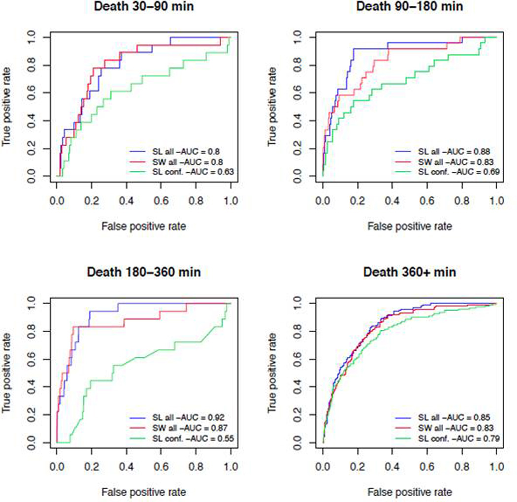
ROC curves showing cross-validated prediction accuracy for SL for the 4 time intervals, comparing performance using just the confounders (C,W; SL Conf.) with fit using all clinical variables of interest, confounding variables, and indicators of missingness (A,W,C) for SuperLearner (SL all) and stepwise regression (SW all)

Variable Importance

The equivalent variable importance results of the three models fit to predict death (semiparametric via SL, stepwise regression, and unadjusted) for pre-specified increases in the predictors reporting either θ_ATE for binary variables, or θ₂ for continuous variables, are shown in Table 2. The importance of variables changes quite dramatically in magnitude and significance from one time point to another; what is a significant predictor for the earliest time point can be a relatively unimportant predictor for death, among those living, at later time points. In addition, whereas the estimates of importance can be also substantively different than those derived by a naïve method (see results for same parameter estimate derived from simple model with stepwise regression), suggesting that misspecification of the model could be contributing significantly to biased estimates of the time-dependent importance of particular variables.

Table 2.

Variable Importance Analysis, θ_ATE for binary, θ₂ for continuous), for death (with p-values), where Delta (δ_A) is the chosen potential change in the corresponding variable of interest for estimates of θ₂, and binary indicates that the variable is binary and thus the θ_ATE estimate is reported. The highlighted sections are discussed in the text.

		30–90 Minutes			90–180 Minutes			180–360 Minutes			360+ minutes
Variable	Delta/binary	Double Robust	Stepwise	Unadjusted	Double Robust	Stepwise	Unadjusted	Double Robust	Stepwise	Unadjusted	Double Robust	Stepwise	Unadjusted
bdresed	0.1	−3.5E-3 (0.16)	−2.2E-4 (0.01)	−2.3E-4 (<0.01)	7.9E-4 (0.73)	−1.6E-4 (0.14)	−2.6E-4 (<0.01)	−2.0E-3 (0.44)	−2.4E-4 (0.64)	−2.6E-4 (0.01)	1.1E-2 (0.01)	−4.5E-4 (0.09)	−3.5E-4 (0.2)
ctubeed	binary	5.4E-3 (0.59)	2.0E-2 (0.7)	2.6E-2 (0.02)	1.3E-2 (0.18)	3.9E-2 (0.46)	5.1E-2 (<0.01)	−2.1E-2 (0.04)	−3.4E-5 (1)	2.0E-3 (0.85)	−1.2E-1 (<0.01)	8.3E-3 (0.75)	4.6E-2 (0.11)
fastresed	binary	−1.2E-2 (0.32)	−1.3E-4 (0.99)	2.5E-3 (0.79)	−1.6E-2 (0.19)	1.0E-2 (0.45)	1.4E-2 (0.33)	−3.6E-3 (0.77)	1.3E-2 (0.31)	1.6E-2 (0.19)	−1.6E-1 (<0.01)	−2.7E-2 (0.27)	−3.5E-2 (0.23)
fibrresed	1	1.4E-2 (0.02)	−1.2E-4 (0.43)	−2.2E-4 (0.1)	1.4E-2 (0.04)	−4.4E-4 (0.03)	−4.8E-4 (0.02)	1.3E-3 (0.84)	−9.3E-5 (0.79)	−1.2E-4 (0.39)	2.9E-2 (0.04)	−5.7E-4 (0.02)	−7.0E-4 (<0.01)
gcsed	1	−4.3E-4 (0.92)	−1.7E-3 (0.59)	−2.5E-3 (0.07)	−2.1E-4 (0.96)	−2.7E-3 (0.06)	−2.9E-3 (<0.01)	−6.2E-3 (0.2)	−3.2E-3 (0.1)	−3.1E-3 (<0.01)	3.6E-4 (0.97)	−1.3E-2 (<0.01)	−1.8E-2 (<0.01)
glued	3.4	1.1E-3 (0.28)	4.9E-4 (0.22)	5.5E-4 (<0.01)	−2.4E-4 (0.77)	3.6E-4 (0.03)	4.4E-4 (0.01)	−6.5E-6 (0.97)	4.2E-4 (0.05)	4.3E-4 (<0.01)	3.5E-3 (0.04)	1.2E-3 (0.02)	1.3E-3 (0.01)
hctresed	1	−3.5E-3 (<0.01)	−2.2E-3 (0.01)	−2.4E-3 (<0.01)	6.9E-4 (0.88)	−6.2E-4 (0.68)	−1.1E-3 (0.12)	−3.2E-3 (<0.01)	−6.1E-4 (0.29)	−7.6E-4 (0.14)	−8.6E-3 (0.22)	1.5E-4 (0.93)	−7.1E-4 (0.64)
hgbresed	0.1	−1.1E-3 (0.2)	−7.3E-4 (0.2)	−7.5E-4 (<0.01)	−3.7E-4 (0.21)	−4.6E-4 (0.72)	−5.2E-4 (0.01)	−2.9E-4 (0.48)	−2.4E-4 (0.2)	−2.6E-4 (0.07)	−3.9E-6 (1)	2.3E-4 (0.66)	−2.5E-4 (0.61)
hred1	1	3.0E-4 (0.82)	−3.8E-5 (0.84)	−4.9E-5 (0.8)	1.2E-3 (0.17)	2.0E-4 (0.47)	1.2E-4 (0.63)	1.3E-4 (0.92)	1.7E-4 (0.44)	1.2E-4 (0.57)	1.2E-3 (0.14)	1.8E-4 (0.69)	−1.2E-4 (0.83)
inrresed	0.1	−2.3E-3 (0.57)	2.7E-4 (1)	3.5E-4 (0.06)	1.4E-2 (0.17)	4.1E-4 (1)	4.6E-4 (0.1)	2.1E-2 (0.27)	6.6E-5 (0.9)	1.2E-4 (0.44)	2.0E-2 (0.06)	6.9E-4 (0.34)	1.3E-3 (0.15)
intubed	binary	−1.3E-2 (0.21)	4.5E-3 (0.64)	8.5E-3 (0.43)	−1.8E-3 (0.87)	2.5E-2 (0.09)	3.4E-2 (0.03)	2.2E-2 (0.06)	4.2E-2 (0.02)	4.5E-2 (<0.01)	−1.2E-1 (<0.01)	2.9E-2 (0.28)	5.7E-2 (0.07)
iss	1	3.1E-4 (0.76)	7.1E-4 (0.04)	7.3E-4 (0.04)	2.0E-3 (0.22)	1.2E-3 (<0.01)	1.2E-3 (<0.01)	6.4E-5 (0.96)	3.9E-4 (0.86)	4.9E-4 (0.04)	1.8E-2 (<0.01)	4.7E-3 (<0.01)	5.1E-3 (<0.01)
ndecomed	binary	9.1E-2 (0.25)	1.1E-1 (0.3)	2.1E-1 (0.15)	−4.8E-2 (<0.01)	−2.6E-2 (0.05)	−2.5E-2 (<0.01)	4.4E-2 (0.52)	1.5E-1 (0.3)	1.2E-1 (0.47)	8.8E-2 (0.58)	7.1E-2 (0.68)	2.0E-1 (0.29)
plasmasum	1	1.1E-2 (0.11)	2.1E-3 (0.09)	3.0E-3 (0.01)	7.8E-3 (0.11)	4.2E-3 (<0.01)	4.7E-3 (<0.01)	1.5E-2 (<0.01)	5.2E-3 (<0.01)	4.8E-3 (<0.01)	3.3E-2 (<0.01)	1.4E-2 (0.02)	1.6E-2 (<0.01)
pltresed	4	−6.3E-4 (<0.01)	−5.7E-4 (0.25)	−6.9E-4 (0.02)	−1.0E-3 (0.05)	−1.1E-3 (0.15)	−9.9E-4 (<0.01)	−8.9E-4 (0.19)	−4.1E-4 (0.54)	−4.9E-4 (0.03)	−1.6E-3 (0.21)	−6.0E-4 (0.34)	−1.5E-3 (0.06)
pltsum	1	−7.8E-3 (0.32)	−1.3E-3 (0.75)	4.6E-4 (0.93)	−7.9E-3 (0.5)	1.7E-3 (0.37)	4.1E-3 (0.04)	9.1E-3 (0.18)	5.1E-3 (<0.01)	4.9E-3 (<0.01)	1.3E-2 (0.38)	9.0E-3 (0.11)	1.4E-2 (<0.01)
RBCsum	1	3.8E-3 (0.09)	1.7E-3 (0.06)	2.4E-3 (<0.01)	7.7E-3 (<0.01)	3.3E-3 (<0.01)	3.9E-3 (<0.01)	2.0E-3 (0.48)	2.9E-3 (0.63)	2.9E-3 (<0.01)	1.5E-2 (0.16)	6.7E-3 (0.02)	8.5E-3 (<0.01)
rfviiaed	binary	−4.1E-2 (<0.01)	0.0E+0 (1)	−1.9E-2 (<0.01)	−4.2E-2 (<0.01)	−2.5E-2 (0.03)	−2.5E-2 (<0.01)	−2.4E-2 (0.01)	−1.9E-2 (0.57)	−1.9E-2 (<0.01)	−7.1E-2 (0.74)	4.1E-2 (0.82)	1.5E-1 (0.4)
sbped1	1	−1.6E-3 (0.18)	−2.0E-4 (0.21)	−2.3E-4 (0.17)	−2.0E-4 (0.58)	8.9E-5 (0.6)	1.4E-4 (0.49)	−1.1E-3 (0.31)	−6.4E-5 (0.69)	−7.2E-5 (0.72)	2.6E-4 (0.81)	4.0E-4 (0.24)	3.7E-4 (0.35)
sked	1	3.8E-3 (0.71)	4.7E-3 (0.49)	7.9E-3 (0.31)	2.5E-2 (0.16)	1.9E-2 (0.05)	2.5E-2 (0.03)	1.0E-2 (0.42)	1.0E-2 (0.24)	1.3E-2 (0.17)	−3.0E-2 (0.07)	−4.8E-3 (0.75)	2.0E-2 (0.29)
snaed	1	−5.1E-3 (<0.01)	−2.7E-4 (0.63)	−1.8E-4 (0.8)	6.3E-3 (0.52)	−8.2E-5 (0.9)	−1.0E-4 (0.89)	−1.8E-4 (0.98)	7.1E-4 (0.32)	8.4E-4 (0.24)	−6.5E-3 (0.72)	6.6E-4 (0.72)	5.3E-4 (0.82)
toured	binary	−1.8E-3 (0.94)	1.1E-2 (0.77)	8.2E-3 (0.77)	−4.5E-2 (<0.01)	−2.6E-2 (<0.01)	−2.6E-2 (<0.01)	−4.6E-3 (0.81)	3.7E-2 (0.33)	3.6E-2 (0.33)	−2.0E-1 (<0.01)	−4.1E-2 (0.5)	−8.1E-2 (0.05)
traxred	binary	1.5E-4 (0.99)	2.4E-2 (0.68)	2.4E-2 (0.49)	−2.9E-2 (0.02)	−2.5E-3 (0.99)	−3.5E-3 (0.88)	−1.8E-2 (0.28)	−6.4E-4 (0.98)	3.1E-3 (0.89)	−1.6E-1 (<0.01)	−7.9E-3 (0.87)	2.5E-2 (0.69)

Discussion

We present here the first application of SL and associated variable importance techniques to multivariate data prospectively collected in real time from severely injured trauma patients. While this application represents a first proof of concept study for application of these computational techniques to noisy patient data, our findings suggest that these models find very good prediction of the outcomes of death (ROC curves .8 –.92). In addition to overall prediction of future mortality, these results also allow discrimination of the relative predictive ability of baseline patient or injury characteristics (which have poor predictive capability) and those variables for which the semiparametric associations we report suggest more evidence for important targets of intervention, or at least a subset for which one can build an accurate prognostic score. This discrimination by itself allows for clinical inference of how much of a patient’s outcome is based on recorded injury characteristics, which are not subject to intervention, versus how much can be intervened upon, representing potentially improved outcomes. This analysis is then extended and augmented by the variable importance analysis, which provides insight as to the specific drivers of a given outcome each different time interval. This is particularly important as this represents what clinicians implicitly know: patients change over time and patients will need different interventions due to these physiologic changes. Together then these statistical techniques represent the entire thought process of the clinician; prediction which changes over time, given the current data available and a focus on variables believed most responsible for a patient’s prognosis.

To implement this strategy, we rely on procedures that have theoretical justification under a semiparametric model. Thus, for prediction, we rely on an ensemble learner (a method based on cross-validation, which can combine both simple regression models as well as more sophisticated model selection/prediction methods), which is based both on practical performance, but also statistical theory. As described, this leads to the so-called SL approach, and we report the overall performance of this predictor, for time specific hazard of death. Our results show that we never do worse than much smaller, admittedly simpler procedures, and in several cases, we have better performance, precisely as predicted by the Oracle Inequality^10,15. In addition, the resulting predictors served as the basis for estimating the importance of the candidate predictors in their potential to explain variability in the outcome, what we called estimation of variable importance measures (VIM). Because the fact that the resulting prediction models derive from a procedure that guarantees (at least in the limit) that the “best” candidate is chosen, we argue that VIM’s should be relatively efficient (i.e., lower mean-squared error) compared to those based on arbitrarily chosen parametric (e.g., simple logistic regression) models. In addition, the parameters defining VIM’s, which are derived from the causal inference literature, have been chosen to provide clinically meaningful measures of potential interventions (e.g., the impact on rate of death for theoretically increasing the use of a particular blood product). As in the prediction, the methodology used for VIM’s also has proven optimality properties, so that we avoid ad hoc rationales and also potentially biased inference from such ad hoc procedures, including overly optimistic measures of fit. . We finally note that this procedure can be used as validation of more traditional parametric models by including them as competitors (as was done for this analysis) and if the data show they are a superior fit, then both the prediction model and the resulting VIM derived from these will match what is returned by our approach.

We have included such models within our ensemble SL predictor, and compared the results to one of these more standard results, which sometimes derive very different estimates of the time-dependent estimates of variable importance; examination of the variable importance measures for prediction of death in the first 90 minutes reveals that lower initial hematocrit, platelets, and fibrinogen and sodium are predictive of death. Put into clinical context a 1 point increase in hematocrit decreases the likelihood of death by .03%. Interestingly the administration of rVIIa which in this cohort is an unusual occurrence was in fact protective suggesting that either the drug was effective or was associated with aggressive care that benefited patients. During the second time interval (90 to 180 minutes), lower initial ED platelet count and fibrinogen levels remained associated with increased mortality while initial hematocrit is no longer a predictor of future death. Hemostatic interventions including placement of a tourniquet in the ED, and the administration of rVIIa were protective. For each additional RBC unit given to this time point the likelihood of mortality increased by nearly 1% which would be expected as increased transfusion need has been shown to be associated with worse outcome.

Of greatest interest lies in the changing predictors of outcome in the context of robust prediction (AUC curves predicting death of >.85). Common physiologic predictors are sometimes predictive and other times the variable importance implies, for this data, less if any information. The results support the broader use of such techniques, in that in most cases, the predictors are in the correct statistical direction and estimates of the impact of (known) life saving interventions were typically found to be predictive. In addition, these techniques can produce diagnostic scores that can be used in real time by physicians, where one concentrates only on those variables practically accessible at critical early moments after a patients injury, and these scores can change in time given the evolving relationship of early indicators and their prognostic ability, given the evolution of the patient and the target population (e.g., attrition by death).

Taken together these examples provide insight about how variable importance can provide insight into the changing drivers of highly predictable outcomes over time. The next step is to derive plots of the dose response curves for each variable for each outcome to show the effect for each increment across the distribution of a variable on an outcome. Because it is likely that most of the true dose-response curves have some degree of non-linearity, these types of summary measures reported for continuous variables obscure the fact that the same theoretical intervention will have different impacts on different patients at different times (i.e., patients starting at different levels of the variable of interest). However, the approach followed here does not assume such a linear (or any) does-response and so at least the summary measure is not dependent on a pre-specifying an arbitrary (and thus misspecified) model. In subsequent studies, we will estimate similar parameters as reported here, as well as the dose-response equivalents, so that we can examine the distribution of how these potential interventions change as the baseline characteristics of the patients change. This highlights the great strength of this approach; it can tailor the parameter to the specific clinical goals of the study (e.g., the impacts of “dynamic” treatments), whereas using flexible techniques that are capable of optimal bias-variance trade-offs in fitting the statistical model of the data. If a simpler, more traditional regression model is sufficient to fit the data, these methods will produce equivalent estimates as these techniques, so that one does not lose by using a more aggressive, machine learning methodology with subsequent targeted estimation of parameters with potential clinical relevance.

References Cited

- 1.Injury Chart Book. Geneva: World Health Orginization; [Google Scholar]
- 2.Hess JR, Holcomb JB, Hoyt DB. Damage control resuscitation: the need for specific blood products to treat the coagulopathy of trauma. Transfusion. 2006;46:685–686. doi: 10.1111/j.1537-2995.2006.00816.x. [DOI] [PubMed] [Google Scholar]
- 3.Holcomb JB, McMullin NR, Pearse L, Carusa J, Wade CE, Oetjen-Gerdes L, Champion HR, Lawnick M, Farr W, Rodriguez S, et al. Causes of death in U.S. Special Operations Forces in the global war on terrorism: 2001–2004. Ann Surg. 2007;245:986–991. doi: 10.1097/01.sla.0000259433.03754.98. [DOI] [PMC free article] [PubMed] [Google Scholar]
- 4.Krumrei NJ, Park MS, Cotton BA, Zielinski MD. Comparison of massive blood transfusion predictive models in the rural setting. J Trauma Acute Care Surg. 2012;72:211–215. doi: 10.1097/TA.0b013e318240507b. [DOI] [PMC free article] [PubMed] [Google Scholar]
- 5.Lesko MM, Jenks T, O'Brien S, Childs C, Bouamra O, Woodford M, Lecky F. Comparing Model Performance for Survival Prediction Using Total GCS and Its Components in Traumatic Brain Injury. J Neurotrauma. 2012 doi: 10.1089/neu.2012.2438. [DOI] [PubMed] [Google Scholar]
- 6.Macfadden LN, Chan PC, Ho KH, Stuhmiller JH. A model for predicting primary blast lung injury. J Trauma Acute Care Surg. 2012;73:1121–1129. doi: 10.1097/TA.0b013e31825c1536. [DOI] [PubMed] [Google Scholar]
- 7.Nunez TC, Voskresensky IV, Dossett LA, Shinall R, Dutton WD, Cotton BA. Early prediction of massive transfusion in trauma: simple as ABC (assessment of blood consumption)? J Trauma. 2009;66:346–352. doi: 10.1097/TA.0b013e3181961c35. [DOI] [PubMed] [Google Scholar]
- 8.Schochl H, Cotton B, Inaba K, Nienaber U, Fischer H, Voelckel W, Solomon C. FIBTEM provides early prediction of massive transfusion in trauma. Crit Care. 2011;15:R265. doi: 10.1186/cc10539. [DOI] [PMC free article] [PubMed] [Google Scholar]
- 9.Buchman TG. Novel representation of physiologic states during critical illness and recovery. Critical Care. 2010;14:127. doi: 10.1186/cc8868. [DOI] [PMC free article] [PubMed] [Google Scholar]
- 10.van der Laan MJ, Polley EC, Hubbard AE. Super learner. Stat Appl Genet Mol Biol. 2007;6 doi: 10.2202/1544-6115.1309. Article 25. [DOI] [PubMed] [Google Scholar]
- 11.van der Laan M, Rose S. Targeted learning: causal inference for observational and experimental data. New York: Springer; 2011. [Google Scholar]
- 12.Rahbar MH, Fox EE, del Junco DJ, Cotton BA, Podbielski JM, Matijevic N, Cohen MJ, Schreiber MA, Zhang J, Mirhaji P, et al. PROMMTT Investigators. Coordination and management of multicenter clinical studies in trauma: Experience from the PRospective Observational Multicenter Major Trauma Transfusion (PROMMTT) Study. Resuscitation. 2012;83:459–464. doi: 10.1016/j.resuscitation.2011.09.019. [DOI] [PMC free article] [PubMed] [Google Scholar]
- 13.Rubin DB. Bayesian Inference for causal effects: the role of randomization. Ann Stat. 1978;6:34–58. [Google Scholar]
- 14.Ihaka R, Gentleman R. R: A Language for Data Analysis and Graphics. J Comp Graphical Stat. 1996;5:299–314. [Google Scholar]
- 15.van der Laan MJ, Rubin DB. Targeted maximum likelihood learning. Int J Biostat. 2006;2 doi: 10.2202/1557-4679.1211. [DOI] [PMC free article] [PubMed] [Google Scholar]
- 16.Gelman A, Jakulin A, Pittau MG, Su Y-S. A weakly informative default prior distribution for logistic and other regression models. Ann Appl Stat. 2008;2:1360–1383. [Google Scholar]
- 17.Friedman J, Hastie T, Tibshirani R. Regularization Paths for Generalized Linear Models via Coordinate Descent. J Stat Softw. 2010;33:1–22. [PMC free article] [PubMed] [Google Scholar]
- 18.Breiman L. Random forests - random features. Berkeley: Department of Statistics, University of California; 1999. [Google Scholar]
- 19.Pearl J. Causality. Cambridge: Cambridge University Press; 2000. [Google Scholar]
- 20.Munoz ID, van der Laan M. Population Intervention Causal Effects Based on Stochastic Interventions. Biometrics. 2012;68(2):541–549. doi: 10.1111/j.1541-0420.2011.01685.x. [DOI] [PMC free article] [PubMed] [Google Scholar]
- 21.Efron B, Tibshirani RJ. An Introduction to the Bootstrap. Boca Raton, FL: Chapman & Hall, CRC; 1993. [Google Scholar]
- 22.Polley E, van der Laan M. SuperLearner: Super Learner Prediction. R package version 2.0–6. 2012 [Google Scholar]
- 23.Hastie T, Tibshirani R. Generalized additive models: An Introduction with R. New York: Chapman and Hall; 1990. [Google Scholar]