Intrinsic noise in gene regulatory networks

Abstract

Cells are intrinsically noisy biochemical reactors: low reactant numbers can lead to significant statistical fluctuations in molecule numbers and reaction rates. Here we use an analytic model to investigate the emergent noise properties of genetic systems. We find for a single gene that noise is essentially determined at the translational level, and that the mean and variance of protein concentration can be independently controlled. The noise strength immediately following single gene induction is almost twice the final steady-state value. We find that fluctuations in the concentrations of a regulatory protein can propagate through a genetic cascade; translational noise control could explain the inefficient translation rates observed for genes encoding such regulatory proteins. For an autoregulatory protein, we demonstrate that negative feedback efficiently decreases system noise. The model can be used to predict the noise characteristics of networks of arbitrary connectivity. The general procedure is further illustrated for an autocatalytic protein and a bistable genetic switch. The analysis of intrinsic noise reveals biological roles of gene network structures and can lead to a deeper understanding of their evolutionary origin.

Noise is often perceived as being undesirable and unpredictable; however, living systems are inherently noisy and are optimized to function in the presence of stochastic fluctuations (1). Some organisms can exploit stochasticity to introduce diversity into a population, as occurs with the lysis–lysogeny bifurcation in phage λ (2) or the DNA inversion mechanism in bacteria (3). In contrast, stability against fluctuations is essential for the case of a gene regulatory cascade controlling cell differentiation in a developing embryo (4). These fluctuations are intrinsic: they are determined by the structure, reaction rates, and species concentrations of the underlying biochemical networks. Here our goal is to quantify the macroscopic statistics of genetic networks given the microscopic rate constants and interactions and to investigate the evolutionary and biological implications of noise.

Several models have been proposed that incorporate stochasticity in gene expression. For example, numerical and analytic methods have been used to investigate stochastic gene induction and repressor action (5–7), and analytic results have been obtained for the stochastic expression of a single gene in eukaryotes (8) and in a growing cell population (9). In living systems, however, groups of genes and proteins work in concert. The introduction of regulatory interactions creates a gene network with complex emergent properties (10). One approach to studying the resulting network noise might involve running detailed numerical simulations incorporating all known reactions, rates, and species. This technique has been used in the analysis of the phage λ lysis–lysogeny decision circuit (2). The numerical predictions match experimental data, but they provide no intuition into underlying correlations and interactions. Analytic results can be obtained by applying the Langevin technique, where the noise source is specified externally (11). However, reconciling external and intrinsic noise becomes a subtle exercise.

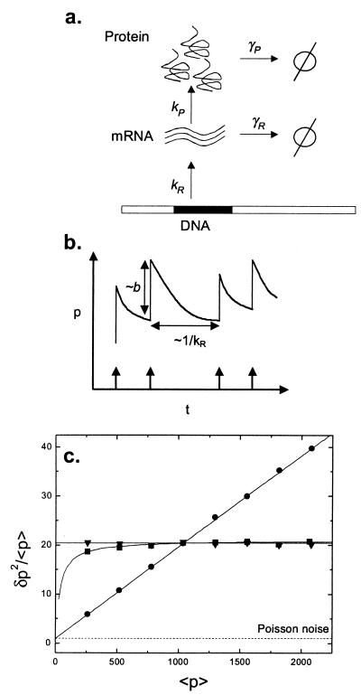
We consider a simple and intuitive model for gene expression in prokaryotes that contains all of the essential features of transcription, translation, and interactions between genes in a regulatory network (see Appendix; Fig. 1a). For simplicity, we do not treat the random partitioning of proteins during cell division. Both the time dependence and the steady-state statistics of this model can be obtained analytically. Here we focus on exploring the mean (<q>) and the variance (δq²) of the number of molecules of each species q in the steady state for several gene regulatory modules. These system properties are simple to understand, clear to interpret, and most importantly, they are easily accessible experimentally.

Figure 1.

Modeling single gene expression. (a) mRNA molecules are synthesized at rate k_R from the template DNA strand. Proteins are translated at a rate k_P off each mRNA molecule. Proteins and mRNA degrade at rates γ_P and γ_R, respectively. Degradation into constituents is denoted by φ. All reactions are assumed to be Poisson, so that the probability of a reaction with rate k happening in a time dt is given by kdt, and the waiting times between successive reactions are exponentially distributed. (b) A simplified timecourse illustrates the intuition behind the result of Eq. 1. Transcription initiation events occur with average frequency k_R and are indicated by arrows; each mRNA transcript releases a burst of proteins of average size b, and proteins decay between bursts. (c) Controlling mean and variance of protein number by varying system parameters for single gene expression. The Fano factor ratio (δp²/<p> ≡ variance/mean) is plotted versus the mean. The mRNA half-life is fixed at 2 min. The base case corresponds to a burst size b = 20, a transcript initiation rate k_R = 0.01 s⁻¹ and a protein half-life ln(2)/γ_P = 1 h. The three curves are produced by varying one of these parameters while keeping the other two fixed. b is varied between 5 and 40 (circles); k_R is varied between 0.0025 s⁻¹ and 0.02 s⁻¹ (triangles); protein half-life is varied from 15 min to 2 h (squares). The Poisson value of δp²/<p> = 1 is marked for comparison. Monte Carlo results (symbols) match analytic values given by Eq. 1 exactly (solid lines).

Theory

Noise Strength.

Noise strength is usually reported in terms of the standard deviation σ of a stochastic variable q. The Fano factor, defined as is related to the standard deviation by because q measures molecule number, ν is a dimensionless quantity. When number fluctuations are because of a Poisson process, we have ν = 1. The Fano factor of an arbitrary stochastic system reveals deviations from Poissonian behavior. It is a sensitive measure of noise and the unit in which we report our results.

Network Model.

The biochemical genetic system is assumed to be specified at any time t by the total number of mRNA molecules (r) and protein molecules (p) present. We neglect other state variables such as various configurations of the DNA operator region (e.g., free or bound to a repressor), the mRNA molecule (e.g., ribosome occupancy), and the protein (e.g., partially folded states). Such approximations are valid for reasonable parameter ranges (see Appendix).

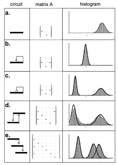
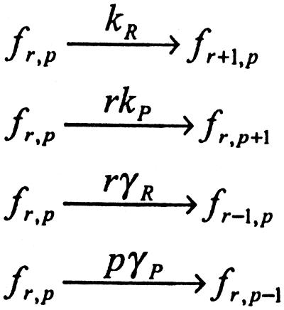
For the simple case of single gene expression, mRNA molecules are synthesized constitutively off the template DNA strand and are translated at some constant rate (Figs. 1a and 4a). The probability that the system is in a given state {r,p} is specified by the joint probability distribution f_r,p (t) that evolves according to Scheme S1:

Figure 4.

Analysis of various gene regulatory networks. (a) Single gene. (b) Autoregulatory protein. Parameters are the same as in a but with repression turned on. (c) Autocatalytic protein. Both steady states are shown. (d) Bistable switch with two mutually repressing proteins. This system occasionally makes a transition from one steady state to the other, leading to a shallow valley between the two peaks not predicted by the analytic model. (e) Feed-forward cascade of three genes. A histogram is shown for each protein. In each case, the network is represented schematically and the network matrix A is shown (with entries + or − showing the sign of each quantity). The matrix Γ is omitted because it is always diagonal. The results from a typical Monte Carlo simulation of the network are shown. The numerical histograms for protein number are overlaid with Gaussians (solid lines), with the mean and variance predicted by the analytic model.

Scheme 1.

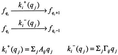
For the case of a gene network with many interacting species indexed by i, the phase space generalizes to {r_i,p_i}, and the rate constants go over to k_Ri, k_Pi, γ_Ri, γ_Pi. We can specify network connectivity by making the reaction rates (possibly nonlinear) functions of the state of the system. In the simplest case, when these rates are constant, Scheme S1 is a special case of Scheme S2, shown below, where the rates are taken to be linear functions of the state variables {q_i}:

Scheme 2.

Here, A shows how the rate of creation of species i is influenced by the number of molecules of species j. Similarly, Γ gives the rate of destruction of species i in terms of the number of molecules of species j. To obtain Scheme S1 from Scheme S2, let the species q_i range over the DNA (D), mRNA molecules (r), and proteins (p). That is: {q_i} = {D, r, p}. The matrices A and Γ for single gene expression are:

Γ is typically diagonal because the rate of decay of species i usually depends only on the number of molecules of i present. The steady-state statistics of Scheme S2 are obtained as solutions of simple linear equations involving the A and Γ matrices (see Appendix).

Results

Single Gene.

The single gene is the fundamental module of gene regulatory circuits. Fluctuations in the concentration of a single gene product are significant because they will affect multiple regulatory processes. In steady state, the mRNA molecules equilibrate independent of the protein molecules and reach a Poisson distribution with <r> = k_R/γ_R and δr²/<r> = 1. The rate of creation of proteins, however, depends on the number of mRNA molecules present. Protein numbers have a distribution that is much broader than Poisson:

1

where η = γ_P/γ_R is the ratio of mRNA to protein lifetimes, and b = k_P/γ_R is the average number of proteins produced per transcript. Between the synthesis and degradation of an mRNA molecule, it is translated by ribosomes, releasing a burst of proteins into the cytoplasm. It can be demonstrated for this model that the number of proteins in each burst is geometrically distributed, with average value b (refs. 9 and 12; Fig. 1b). Typical values for b are 40 for lacZ and 5 for lacA (13). mRNA molecules usually decay much faster than proteins, so η is typically a small quantity. Eq. 1 shows that the width of the protein distribution in this approximation is determined primarily by the average burst size b: intrinsic noise is controlled at the translational level.

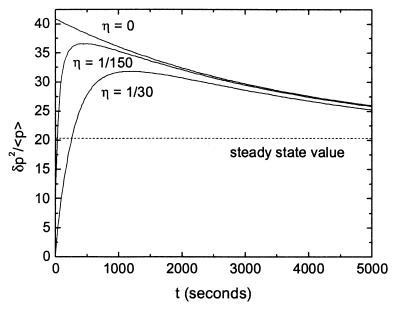
The time dependence of Scheme S1 can be obtained exactly and reveals that noise for a single gene system out of equilibrium is stronger than noise at steady state. Consider a system in which the gene is induced at time t = 0. In the limit that η goes to zero, the system evolves according to:

2

Roughly, the variance δp² relaxes to its steady-state value at a rate 2γ_Pt, twice as quickly as the mean. For small times, δp²/<p> ≅ 2b + 1 is almost twice the steady-state value. Fig. 2 illustrates this transient noise behavior and compares the exact result for finite η to the simplified result of Eq. 2.

Figure 2.

Transient noise for a single gene. The protein half-life is fixed at 1 h, b = 20, and k_R = 0.01 s⁻¹. Exact analytic results are plotted for an mRNA half-life of 120, 24, and 0 s, corresponding to η = 1/30, 1/150, and 0, respectively. δp²/<p> is plotted versus time in seconds. The η = 0 case corresponds to Eq. 2; the steady-state value from Eq. 1 is shown as a dashed line. The transient noise reaches almost twice the steady-state strength, as η tends to zero.

Autoregulatory System.

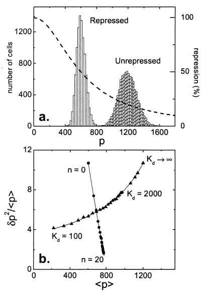
Autoregulation is a ubiquitous motif in biochemical pathways, essential in the management of protein and chemical concentrations through feedback (ref. 14; Figs. 3 and 4b). Autoregulation can be modeled by taking the rate of transcript initiation to be a nonlinear decreasing function of protein concentration, such as a Hill repression function (Fig. 3a). In steady state, the distribution of protein number has a finite width and samples only a small region of the repression curve (Fig. 3a). In that region, the function is well approximated by its linearization about the mean value of p: k_R ≅ k₀ −k₁p. The network matrices for the autoregulatory system are:

These produce the following protein number statistics:

3

where b and η are as defined previously, and φ = k₁/γ_P describes the strength of the negative feedback. Eq. 3 shows that autoregulation has an effect not only in controlling the protein concentration but also in reducing the relative size of fluctuations. Fig. 3b compares the predictions of this model to the results of Monte Carlo simulations of the fully nonlinear system; the match is excellent.

Figure 3.

Noise control by autoregulation. (a) The histogram (scale on left axis) to the right shows the unrepressed distribution, the one to the left the distribution when repression is turned on. The rate of protein production at any given protein number p is given by a Hill repression function (dashed line, scale on right axis): k_R/k=1/(1+[p/K_d]”). Here, K_d is the dissociation constant that specifies the threshold protein concentration at which the transcription rate is at half its maximum value. n is the Hill coefficient and determines the steepness of the repression curve. For example, the cI repressor protein acts on the promoters P_R and P_RM of phage λ with a K_d of about 50 and 1,000 nM, respectively (26). Typical biological values for n range from 1 (hyperbolic control) to over 30 (sharp switching). Note that the repression curve is very nearly linear in the region where it intersects the repressed histogram. (b) Noise control by autoregulation: comparing analytic results (solid lines, Eq. 3) with Monte Carlo simulations, as K_d is varied (triangles), and n is varied (circles). As in Fig. 1c, the Fano factor (variance/mean) is plotted versus the mean. The protein half-life is fixed at 1 h, mRNA half-life at 2 min, and the burst size at 10; the unrepressed mean value is <p>_unrep = 1,200. Note that n = 0 corresponds to a fixed transcription initiation rate that is half the base value, therefore giving a mean protein number of 600. K_d is varied (triangles) from 100 to 2,000 in increments of 100, and then from 2,000 to 5,000 in increments of 1,000, with n set to 2. (K_d is given in molecule number; one molecule per cell corresponds to a concentration of ≈1 nanomolar.) The unrepressed (K_d is infinite) limit is also shown. n is varied (circles) from 0 to 20, with K_d set at 800. The Monte Carlo simulations (symbols) are very well reproduced by the analytical values (solid lines) given by Eq. 3.

Extension to Complex Networks.

Bistability is an important feature of several gene regulatory structures (2). An autocatalytic system, in which a protein enhances its own production (Fig. 4c), typically has two stable states: one at low protein concentrations, where protein creation is near its basal level, and another at high protein concentrations. This is the “all-or-none” phenomenon seen for autocatalytic systems such as the ara (15) and lac (16) operons. A bistable switch can also be constructed from two mutually repressing proteins (ref. 17; Fig. 4d). Fig. 4 shows how the noise analysis would proceed for the systems discussed here, as well as for a feed-forward cascade of three genes (Fig. 4e). These examples indicate how the theory can be applied to arbitrary regulatory networks. In the general case, nonlinear interactions between various species typically lead to multiple stable fixed points; each such fixed point induces a distinct linearized system, and the linearized systems can be solved by using analytic theory.

Range of Validity of the Analytic Model.

First, cell division and the random partitioning of proteins between daughter cells are a source of stochastic fluctuations that will modify the results presented above. For example, Berg (9) has analyzed the expression of a single gene in a dividing cell population (in the absence of protein degradation). He calculates the Fano factor as a function of cell age t in a population with cell division time T:

4

This implies ν = (4/3)b + 1 just before and ν = (2/3)b + 1 just after cell division, compared with ν=b+1 predicted by our simplified model.

Second, in this paper, we have described a linearized stochastic model. However, biochemical systems are invariably nonlinear. Indeed, it is nonlinearity that creates much of the rich variety of behavior exhibited by biological networks. When the resulting system displays limit cycles or oscillations (e.g., ref. 18), it will not yield to naive linearization. Linearization is also invalid around or near unstable or quasistable (also known as critical) fixed points. For example, the threshold or saddle point of a bistable system (Fig. 4d) is not well approximated by our approach. However, nonlinear networks often display multiple stable fixed points; about these points, linearization is a valid approximation, as with the examples treated above. The range of validity will vary from case to case, with the approximation becoming exact in the limit of small fluctuations.

Third, the biochemical reactions we have described are all birth and death processes with first-order rates. Other types of reactions, such as modifications or second- and higher-order interactions between biochemical species, will introduce stochasticity of a different character. For example, fluctuations in DNA–repressor interactions (7) can contribute significantly to system noise. When such interactions are much faster than the reactions we have considered, they can be treated deterministically and then linearized within our analytic framework.

Finally, we have presented mainly steady-state results, whereas many biologically interesting systems are driven or out of equilibrium. We have shown above that for a single gene, noise out of equilibrium can be significantly higher than that at steady state. Nevertheless, the burst size b enters both Eqs. 1 and 2 in an essential way. In a similar manner, steady-state results for other systems might shed light on their out-of-equilibrium noise properties and will be a useful indicator of their noise characteristics.

Discussion

Noise control can play a major role in determining the structure of gene regulatory networks. For example, Eq. 1 shows that the two-step process of transcription followed by translation has given biochemical circuits the freedom to independently adjust the average concentration of a protein and the spread of that concentration in a population (Fig. 1c). Thus a gene can produce a given protein concentration in two very different ways. At low transcription but high translation rates, few mRNA molecules are synthesized in a cell generation, but each one produces a large variable burst of proteins. This causes significant fluctuations over time and in a population. The same concentration can be achieved with high transcription and low translation rates and therefore a smaller burst size. In this case, many mRNA molecules decay without ever being translated; this procedure is inefficient because high energy phosphate groups are hydrolyzed to drive the synthesis of unused or little-used transcripts. However, inefficient translation results in a steady stream of proteins with much smaller fluctuations. During evolutionary adaptation, living systems have made tradeoffs between energy efficiency and noise reduction in choosing between these two alternatives.

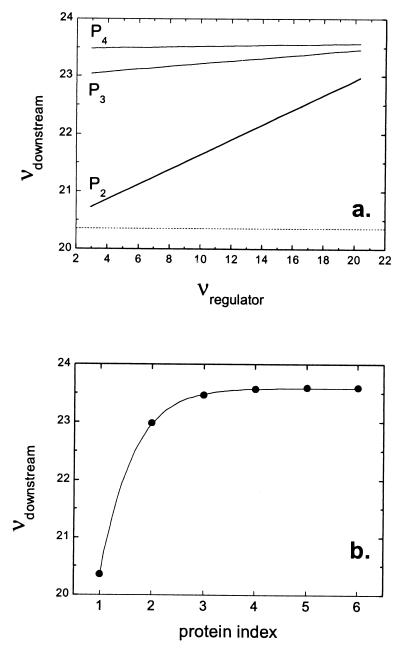
For a regulatory protein that controls the synthesis of several downstream products, fluctuations in regulator concentration will propagate through the cascade (Figs. 4e and 5). Translational noise control is a means by which genetic circuits can reduce noise in such cascades. Regulatory genes such as the cI gene of phage λ (2) and the malT gene of Escherichia coli (19) are often poorly translated. It has been pointed out by other researchers (e.g., ref. 19) that this translational inefficiency might be sustained in the genome through the resulting beneficial reduction in noise. However, we note that in some situations, the intrinsic noise of a regulator can actually increase the sensitivity with which its signal is transmitted (20, 21).

Figure 5.

Propagation of noise in a regulatory cascade. Analytic results are shown for a six gene cascade with gene products P₁, P₂ … P₆ (similar to Fig. 4e). As described below, mean values of all proteins are fixed so that effects purely caused by propagated noise can be seen. P₁ is the regulator protein, P₂ … P₆ are downstream proteins, and i is the protein index of P_i. For all six genes, ln(2)/γ_P = 1 h, ln(2)/γ_R = 2 min. The transcript initiation rate of downstream genes depends hyperbolically on the amount of protein in the previous step of the cascade: k_Ri/k = 1 − 1/(1 + p_i−1/K_d) with K = 500. As in previous figures, we focus on the Fano factor ν = δp²/<P>. (a) For the regulator gene, b is varied from 0 to 20, thereby changing the variance of P₁ (Eq. 1); for downstream genes, b = 20. and are chosen so that P_i = K_d for all i. ν(P₂) … ν(P₄) are plotted against ν(P₁). (Data for i = 5, 6 are difficult to distinguish from those for i = 4.) The predicted value of ν for a burst size b = 20 in the absence of input noise (Eq. 1) is shown as a dashed line. The results indicate that fluctuations in the concentration of a regulatory protein are an important source of noise in a cascade. (b) Now b is fixed at 20 for all genes, and parameters are again chosen so P_i = K_d for all i. ν(P_i) is shown as a function of protein index i. For visual clarity, the results are fitted to a hyperbola. We see that propagated noise makes a significant contribution to the noise of downstream proteins, although saturating after a few steps of the cascade.

The primary function of autoregulation lies in the control of biochemical concentrations in metabolic and genetic pathways. However, we find that it is also a very economical method of noise reduction. Translational noise control is wasteful in that only a small fraction of mRNA molecules are successfully translated into proteins. In contrast, in an autoregulatory system, mRNA molecules are synthesized only when required and are then efficiently translated. Eq. 3 shows that even linear autoregulation can dramatically reduce fluctuations in protein number, down to a small fraction of the unregulated value. Although this result is intuitive and has been directly observed experimentally (14), it is not explicitly predicted by methods such as stability analysis (14) or Langevin analysis; a systematic treatment of intrinsic noise is essential for understanding biologically relevant system properties.

Although stochasticity is evident even in the expression of a single gene, the behavior of a system of genes can be understood only by treating the network as a whole. The analytic model used here provides a quick accurate estimate of the emergent noise properties of genetic networks preferable to that provided by long numerical simulations. The predictions of the model can be used in the design of quantitative experiments in stochastic gene expression. The robustness of network motifs like negative feedback can be quickly tested over a range of parameters, and the importance of particular connections to overall network noise can be estimated (Figs. 3–5). Quantifying the intrinsic noise of genetic and biochemical networks in this manner is essential for understanding the design principles of stable and robust synthetic biochemical systems (14, 17). Conversely, living systems could possess novel regulatory structures whose major or sole function is the control or use of noise (7, 20, 21); such structures can be discovered and understood only through the investigation of emergent network noise properties. As with the examples discussed here, studying noise in gene regulatory networks, as their structure and parameters are varied, can provide new insights into their evolutionary origin and biological function.

Appendix

Modeling Gene Expression in Prokaryotes: Biochemical Assumptions.

During transcription initiation, the initial reversible binding of an RNA polymerase (RNAP) to the promoter region and subsequent formation of an open complex achieve rapid equilibrium (22): initiation from the final open complex is the rate-limiting step (23). The amount of free RNAP in a cell is buffered against cell growth and other time variations by a large pool of nonspecifically bound molecules (24). Transcript initiation is therefore assumed to be a pseudofirst-order reaction with rate k_R. Interactions between species in a network are embodied by transacting factors such as repressor proteins. Such regulatory proteins tend to act by binding the promoter region and shielding it from RNAP, as is the case for the lac repressor (25) or for the Cro protein of phage λ (26). These reactions are considered to be in equilibrium and simply change the fraction of RNAP bound as a closed complex, thereby changing the effective rate k_R of transcript initiation (25). Ribosomes can begin binding the newly synthesized ribosome-binding site almost immediately as transcription begins. Analogous to transcript initiation, translation initiation off a single mRNA molecule is assumed to proceed with a pseudofirst-order rate k_P. For most E. coli operons, initiation and elongation rates are such that ribosome queuing does not occur (13, 27). We therefore take each transcription and translation initiation reaction to be independent. Finally, we assume that mRNA and protein molecules degrade with rates γ_R and γ_P, respectively. A decay rate γ gives a half-life of ln(2)/γ. If growth in cell volume is exponential, rising as e^kt, the resulting dilution of species concentrations can be incorporated by replacing γ_i with γ_I + k for all species i (other than the DNA, which is replicated at a rate exactly matching cell growth). The mRNA decay rate depends on the ribosome-binding rate, because actively translating ribosomes shield the mRNA molecule from the action of nucleases (12, 27).

Construction and Solution of the Master Equation.

Scheme S2 generates the following Master Equation:

A1

where E is the step operator (28) defined by Ef(q_i, …) = f(q_i + k, …). For simplicity, the joint probability distribution is written simply as , indexing the variable of interest by i ranging from 1 to n, the number of species. This equation is linear in the state variables {q_j} and can be solved by constructing the moment generating function Simplify to the case where Γ is diagonal: Γ_ij = δ_ijΓ_j. The function F then obeys the equation

A2

where F_j denotes In steady state, . We now use the following properties of the moment generating function: where signifies evaluation of F at z_j = 1 for all j. Successive differentiation of Eq. A2 will generate linear equations for successively higher moments. Define the vector J_j = F_j and the matrix K_ij= F_ij(where subscripts on F denote differentiation). Differentiating up to second moments gives:

A3

where L_{ij =} A_ijJ_j (no summation). These linear equations can be solved for means (J) and variances (K).

Monte Carlo Simulations.

Simulations were implemented by using Gillespie's algorithm for stochastic coupled chemical reactions (29). The reactions simulated were precisely those shown in Scheme S1 with multiple species, where the reaction rates were allowed to depend nonlinearly on species concentrations. No linearization approximation was used. Steady state was assumed to have been reached at a time equal to 10 times the protein half-life. Each data point or histogram was the result of 10,000 trials.

References

- 1.McAdams H H, Arkin A. Trends Genet. 1999;15:65–69. doi: 10.1016/s0168-9525(98)01659-x. [DOI] [PubMed] [Google Scholar]
- 2.Arkin A, Ross J, McAdams H H. Genetics. 1998;149:1633–1648. doi: 10.1093/genetics/149.4.1633. [DOI] [PMC free article] [PubMed] [Google Scholar]
- 3.van de Putte P, Goosen N. Trends Genet. 1992;8:457–462. doi: 10.1016/0168-9525(92)90331-w. [DOI] [PubMed] [Google Scholar]
- 4.von Dassow G, Meir E, Munro E M, Odell G M. Nature (London) 2000;406:188–192. doi: 10.1038/35018085. [DOI] [PubMed] [Google Scholar]
- 5.Ko M S H. J Theor Biol. 1991;153:181–194. doi: 10.1016/s0022-5193(05)80421-7. [DOI] [PubMed] [Google Scholar]
- 6.Cook D L, Gerber A N, Tapscott S J. Proc Natl Acad Sci. 1998;95:15641–15646. doi: 10.1073/pnas.95.26.15641. [DOI] [PMC free article] [PubMed] [Google Scholar]
- 7.Berg O G, Paulsson J, Ehrenberg M. Biophys J. 2000;79:2944–2953. doi: 10.1016/S0006-3495(00)76531-3. [DOI] [PMC free article] [PubMed] [Google Scholar]
- 8.Peccoud J, Ycart B. Theor Popul Biol. 1995;48:222–234. [Google Scholar]
- 9.Berg O G. J Theor Biol. 1978;71:587–603. doi: 10.1016/0022-5193(78)90326-0. [DOI] [PubMed] [Google Scholar]
- 10.Bhalla U S, Iyengar R. Science. 1999;283:381–387. doi: 10.1126/science.283.5400.381. [DOI] [PubMed] [Google Scholar]
- 11.Hasty J, Pradines J, Dolnik M, Collins J J. Proc Natl Acad Sci USA. 2000;97:2075–2080. doi: 10.1073/pnas.040411297. . (First Published February 18, 2000; 10.1073/pnas.040411297) [DOI] [PMC free article] [PubMed] [Google Scholar]
- 12.McAdams H, Arkin A. Proc Natl Acad Sci USA. 1997;94:814–819. doi: 10.1073/pnas.94.3.814. [DOI] [PMC free article] [PubMed] [Google Scholar]
- 13.Kennell D, Riezman H. J Mol Biol. 1977;114:1–21. doi: 10.1016/0022-2836(77)90279-0. [DOI] [PubMed] [Google Scholar]
- 14.Becskei A, Serrano L. Nature (London) 2000;405:590–593. doi: 10.1038/35014651. [DOI] [PubMed] [Google Scholar]
- 15.Siegele D A, Hu J C. Proc Natl Acad Sci USA. 1997;94:8168–8172. doi: 10.1073/pnas.94.15.8168. [DOI] [PMC free article] [PubMed] [Google Scholar]
- 16.Carrier T A, Keasling J D. J Theor Biol. 1999;201:25–36. doi: 10.1006/jtbi.1999.1010. [DOI] [PubMed] [Google Scholar]
- 17.Gardner T S, Cantor C R, Collins J J. Nature (London) 2000;403:339–342. doi: 10.1038/35002131. [DOI] [PubMed] [Google Scholar]
- 18.Elowitz M B, Leibler S. Nature (London) 2000;403:335–338. doi: 10.1038/35002125. [DOI] [PubMed] [Google Scholar]
- 19.Chapon C. EMBO J. 1982;1:369–374. doi: 10.1002/j.1460-2075.1982.tb01176.x. [DOI] [PMC free article] [PubMed] [Google Scholar]
- 20.Paulsson J, Berg O G, Ehrenberg M. Proc Natl Acad Soc USA. 2000;97:7148–7153. doi: 10.1073/pnas.110057697. . (First Published June 13, 2000; 10.1073/pnas.110057697) [DOI] [PMC free article] [PubMed] [Google Scholar]
- 21.Paulsson J, Ehrenberg M. Phys Rev Lett. 2000;84:5447–5450. doi: 10.1103/PhysRevLett.84.5447. [DOI] [PubMed] [Google Scholar]
- 22.DeHaseth P L, Zupancic M L, Record M T., Jr J Bacteriol. 1998;180:3019–3025. doi: 10.1128/jb.180.12.3019-3025.1998. [DOI] [PMC free article] [PubMed] [Google Scholar]
- 23.Schmitt B, Reiss C. Biochem J. 1995;306:123–128. doi: 10.1042/bj3060123. [DOI] [PMC free article] [PubMed] [Google Scholar]
- 24.McClure W R. Ann Rev Biochem. 1985;54:171–204. doi: 10.1146/annurev.bi.54.070185.001131. [DOI] [PubMed] [Google Scholar]
- 25.Schlax P J, Capp M W, Record M T., Jr J Mol Biol. 1995;245:331–350. doi: 10.1006/jmbi.1994.0028. [DOI] [PubMed] [Google Scholar]
- 26.Shea M A, Ackers G K. J Mol Biol. 1985;181:211–230. doi: 10.1016/0022-2836(85)90086-5. [DOI] [PubMed] [Google Scholar]
- 27.Yarchuk O, Jacques N, Guillerez J, Dreyfus M. J Mol Biol. 1992;226:581–596. doi: 10.1016/0022-2836(92)90617-s. [DOI] [PubMed] [Google Scholar]
- 28.van Kampen N G. Stochastic Processes in Physics and Chemistry. Amsterdam: North–Holland; 1992. [Google Scholar]
- 29.Gillespie D T. J Phys Chem. 1977;81:2340–2361. [Google Scholar]