Statistically accurate low-order models for uncertainty quantification in turbulent dynamical systems

Abstract

A framework for low-order predictive statistical modeling and uncertainty quantification in turbulent dynamical systems is developed here. These reduced-order, modified quasilinear Gaussian (ROMQG) algorithms apply to turbulent dynamical systems in which there is significant linear instability or linear nonnormal dynamics in the unperturbed system and energy-conserving nonlinear interactions that transfer energy from the unstable modes to the stable modes where dissipation occurs, resulting in a statistical steady state; such turbulent dynamical systems are ubiquitous in geophysical and engineering turbulence. The ROMQG method involves constructing a low-order, nonlinear, dynamical system for the mean and covariance statistics in the reduced subspace that has the unperturbed statistics as a stable fixed point and optimally incorporates the indirect effect of non-Gaussian third-order statistics for the unperturbed system in a systematic calibration stage. This calibration procedure is achieved through information involving only the mean and covariance statistics for the unperturbed equilibrium. The performance of the ROMQG algorithm is assessed on two stringent test cases: the 40-mode Lorenz 96 model mimicking midlatitude atmospheric turbulence and two-layer baroclinic models for high-latitude ocean turbulence with over 125,000 degrees of freedom. In the Lorenz 96 model, the ROMQG algorithm with just a single mode captures the transient response to random or deterministic forcing. For the baroclinic ocean turbulence models, the inexpensive ROMQG algorithm with 252 modes, less than 0.2% of the total, captures the nonlinear response of the energy, the heat flux, and even the one-dimensional energy and heat flux spectra.

Turbulent dynamical systems are characterized by both a large dimensional phase space and a large dimension of instabilities (i.e., a large number of positive Lyapunov exponents on the attractor). They are ubiquitous in many complex systems with fluid flow such as, for example, the atmosphere, ocean, and coupled climate system, confined plasmas, and engineering turbulence at high Reynolds numbers. In these, linear instabilities are mitigated by energy-conserving nonlinear interactions that transfer energy to the linearly stable modes where it is dissipated, resulting in a statistical steady state. Uncertainty quantification (UQ) in turbulent dynamical systems is a grand challenge where the goal is to obtain statistical estimates such as the change in mean and variance for key physical quantities in the nonlinear response to changes in external forcing parameters or uncertain initial data. These key physical quantities are often characterized by the degrees of freedom that carry the largest energy or variance, and an even more ambitious grand challenge is to develop truncated low-order models for UQ for a reduced set of important variables with the largest variance. This is the topic of the present paper.

Low-order truncation models for UQ include projection of the dynamics on leading-order empirical orthogonal functions (EOFs) (1), truncated polynomial chaos (PC) expansions (2–4), and dynamically orthogonal (DO) truncations (5, 6). Despite some success for these methods in weakly chaotic dynamical regimes, concise mathematical models and analysis reveal fundamental limitations in truncated EOF expansions (7, 8), PC expansions (9, 10), and DO truncations (11, 12), owing to different manifestations of the fact that in many turbulent dynamical systems modes that carry small variance on average can have important, highly intermittent dynamical effects on the large variance modes. Furthermore, the large dimension of the active variables in turbulent dynamical systems makes direct UQ by large ensemble Monte-Carlo simulations impossible in the foreseeable future while, once again, concise mathematical models (10) point to the limitations of using moderately large yet statistically too-small ensemble sizes. Other important methods for UQ involve the linear statistical response to change in external forcing or initial data through the fluctuation-dissipation theorem (FDT), which only requires the measurement of suitable time correlations in the unperturbed system (13–18). Despite some significant success with this approach for turbulent dynamical systems (13–18), the method is hampered by the need to measure suitable approximations to the exact correlations for long time series as well as the fundamental limitation to parameter regimes with a linear statistical response.

Here a systematic strategy is developed for building statistically accurate low-order models for UQ in turbulent dynamical systems. First, exact dynamical equations for the mean and the covariance are developed; the possibly intermittent effects of the third-order statistics on these low-order statistics are present in the exact equations. Second, an approximate nonlinear dynamical system for the evolution of the mean and covariance is formulated; this system is subjected to the minimal additional damping and additional random forcing so that it has the unperturbed mean and covariance as a stable fixed point. Third, the effect of the third moments on the mean and the covariance in the approximate dynamical system for the statistics are calibrated efficiently at the unperturbed steady state using only the measured first and second moments. The result at this stage is a very recent algorithm for UQ called modified quasilinear Gaussian (MQG) closure (19), which applies on the entire phase space of variables. In the fourth step, the MQG algorithm is projected on suitable leading EOF patterns with further efficient calibration of the effect of the unresolved modes at the unperturbed statistical steady state. This final step defines the reduced-order MQG (ROMQG) method for UQ in turbulent dynamical systems and is developed following the above outline in the next section.

The subsequent sections include two highly nontrivial applications of the ROMQG method in UQ. The first application involves the Lorenz 96 (L-96) model (20, 21), which is a nontrivial 40-dimensional turbulent dynamical system that mimics midlatitude atmospheric turbulence and is a popular model for testing methods for statistical prediction (20), data assimilation or filtering (22), FDT (18), and UQ (11, 12, 19). The advantage of the 40-mode L-96 is that very large ensemble Monte-Carlo simulations can be used for validation in transient regimes. Here the ROMQG algorithm has remarkably robust skill for UQ in the transient response to general random external forcing for truncations as low as one, two, or three leading Fourier modes. The second application involves a prototype example of two-layer ocean baroclinic turbulence (23–25). Here the turbulent system has over 125,000 degrees of freedom, so validation through transient Monte-Carlo simulations is impossible and only the nonlinear statistical steady-state response to the change in shear can be tested for various perturbation levels. Here the ROMQG algorithms for UQ using 252 EOF modes (less than 0.2% of the total modes) are able to capture the nonlinear response of both the one-dimensional energy spectrum and heat flux spectrum at each wavenumber with remarkable skill for a wide range of shear variations. The paper concludes with a brief summary discussion.

Abstract Formulation

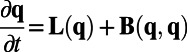
We consider large dimensional turbulent dynamical systems with conservative quadratic nonlinearities with the abstract structural form typically satisfied in applications to geophysical (23–26) or engineering turbulence given by

acting on . In the above equation and for what follows repeated indices will indicate summation. In some cases the limits of summation will be given explicitly to emphasize the range of the index. In the above equation L is a skew-symmetric linear operator, which in geophysics represents rotation, the β-effect of Earth’s curvature, topography, and so on and satisfies . D is a negative definite symmetric operator representing dissipative processes such as surface drag, radiative damping, viscosity, and so forth. The quadratic operator conserves the energy by itself so that it satisfies

in a suitable inner product. Finally, represents the effect of external forcing, for instance solar forcing, which we will assume can be split into a mean component and a stochastic component with white-noise characteristics. In the applications below, the stochastic component of the forcing is zero, although there can be random initial data. We represent the stochastic field through a fixed orthonormal basis , ,

where represent the ensemble average of the response (i.e., the mean field) and the are random processes. The exact mean field equation is given by

with the covariance matrix given by and denotes averaging over the ensemble members ω. The random component of the solution satisfies

By projecting the above equation to each basis element v_i we obtain the exact evolution of the covariance matrix :

where we have

• i) the linear dynamics operator expressing energy transfers between the mean field and the stochastic modes (effect due to B), as well as energy dissipation (effect due to D) and nonnormal dynamics (effect due to L, D, ):

  
• ii) the positive definite operator expressing energy transfer due to external stochastic forcing:

  
• iii) the energy flux between different modes due to non-Gaussian statistics (or nonlinear terms) given exactly through third-order moments:

  

From the conservation of energy property in Eq. 2 it follows that the symmetric matrix Q_F satisfies . These last equations with third-order moments are a potential source of intermittency in the solution of the low-order statistics and need to be modeled carefully in any UQ scheme. This is done next in a minimal, efficient fashion by the MQG method (19).

MQG Models

In typical applications, the unperturbed turbulent dynamical system is defined by constant forcing and there is a statistical steady-state solution with mean and covariance satisfying the steady-state statistical equations in Eqs. 3 and 4 with vanishing time-derivatives. Furthermore, the linear operator in Eq. 5 typically has unstable directions as well as stable subspaces with nonnormal dynamics (13–15, 18, 23–27). The statistical steady state exists through a balance driven by the transfer of energy by the nonlinear terms in Eq. 3 and nonnormal linear dynamics from the unstable directions to the stable ones; the nonlinear steady-state covariance exists because the term involving this nonlinearity and the third statistical moments in the statistical steady state precisely balance the effect of the unstable directions in Eq. 4. The MQG dynamical equation for UQ calibrates this essential effect in an efficient, minimal fashion (19). First note that at the statistical steady state of calibration, , is known as a function of the mean and covariance through Eq. 4 at the statistical steady state. In the MQG dynamics we split the nonlinear fluxes into a positive semidefinite part and a negative semidefinite part :

The positive fluxes indicate the energy being “fed” to the stable modes in the form of external chaotic or stochastic noise. On the other hand, the negative fluxes should act directly on the linearly unstable modes of the spectrum, effectively stabilizing the unstable modes. In particular in MQG we represent the negative definite part of the fluxes as additional damping to modify the eigenvalues associated with the Lyapunov Eq. 4 so that these have nonpositive real part for the correct steady-state statistics. To achieve this we represent the negative fluxes as

with defined by the equation

where is the negative semidefinite part of the steady-state fluxes obtained by the equilibrium equation . Eq. 10 essentially connects the negative-definite part of the nonlinear energy fluxes (which is a functional of the third-order statistical moments) with the second-order statistical properties that express energy properties of the system. One can easily verify that in Eq. 10 is given explicitly by

In the MQG dynamics (19), the evolving damping N is given by with f an appropriate nonlinear function. On the other hand, the positive fluxes are computed according to steady-state information, that is, based on the positive semidefinite fluxes The form of this matrix defines the amount of energy that the linearly stable modes should receive in the form of additive noise. The conservative property of the nonlinear energy transfer operator B requires that for all times the zero-trace conservation property is satisfied. This is achieved by choosing the positive fluxes as

These nonlinear fluxes are time-dependent (because depends on time through R); the last formulation guarantees the zero-trace conservation property at every instant of time. These relations substituted into the equations for the mean and covariance in Eqs. 3 and 4 define the minimal MQG dynamics; by construction is a fixed point of this dynamics but is only neutrally stable owing to the minimal character of the decomposition of in Eq. 8. We introduce the small factor with the flux decomposition to render a stable fixed point of the MQG dynamical system (19). In this fashion we obtain the MQG dynamics for the mean and covariance,

where

with q_s and parameters in the MQG dynamics. These MQG dynamics define the first three steps from the introduction of the UQ strategy developed in this paper. As shown in refs. 12 and 19, the MQG algorithm, with a specific, well-motivated choice of q_s and yields excellent performance as a UQ algorithm when tested comprehensively on the 40-mode L-96 model. However, the MQG algorithm is impractical for large dimensional turbulent dynamical systems with because the covariance matrices of order N² are too expensive to evolve directly. This leads to the need for truncated, low-order MQG algorithms, which are developed next.

ROMQG

For the truncation of the dynamics we use s orthogonal eigenvectors of the covariance matrix given by . These can be chosen as EOF modes. We denote these modes with the matrix In this case the reduced covariance that we resolve is connected with the full N-dimensional covariance by the relation

Because the reduced-order covariance contains only a part of the total stochastic energy the influence of the quadratic terms in the mean field equations will be only partially modeled. To represent this effect in the calibration stage, we include additional forcing that will balance this contribution, which is otherwise ignored owing to the truncation. Thus, we have the mean field equation

The value of the additional forcing is determined using statistical steady-state information for the covariance and the mean. In particular we have the equilibrium equation

where this guarantees that is a steady state of the truncated equation in Eq. 17. For the covariance equation governing we use the exact (but reduced-order) equation for the covariance given by

where for and contain both the nonlinear dynamics owing to triad interactions between all modes but also the ignored linear dynamics owing to the truncation. Because contains truncated nonlinear interactions but also nonnormal linear effects we do not expect to satisfy the conservation property because Nevertheless, we can still use steady-state information to model We have

Now we repeat the ideas used in the MQG algorithm described above. By splitting into a positive definite part and into a negative definite part we have the noise, damping pair

The next step is to scale the above energy fluxes. For the additional damping we use the standard scaling from MQG together with small additional damping for stability,

For the positive fluxes, in MQG described earlier we were scaling with the total nonlinear flux of energy. Here we do not have such information because we are modeling the energy (covariance) partially due to the truncation. To this end we will scale with the nonlinear energy fluxes based on the information provided by the reduced-order covariance. The total positive nonlinear energy flux in the statistical steady state is given by and with the standard MQG approximation in general, the energy flux is

Because we do not have information for the full covariance R we will scale with . Moreover, we modify only along the elements of the full covariance that evolve, that is, according to . These approximations give

Note that for the full space with the above expressions reduce exactly to the standard MQG formula. In summary, the ROMQG dynamics are the modified mean equation in Eq. 17 coupled to the reduced covariance equation

with , defined in Eqs. 19 and 20, respectively.

Application of ROMQG to UQ for the L-96 Model

The L-96 model is a discrete periodic model given by

with and with F the deterministic forcing parameter. With the standard discrete Euclidian inner product, one can easily verify that the energy conservation property for the quadratic part is satisfied [i.e., ] and the negative definite part has the diagonal form The model is designed to mimic baroclinic turbulence in the midlatitude atmosphere with the effects of energy conserving nonlinear advection and dissipation represented by the first two terms in Eq. 21. For sufficiently strong constant forcing values such as F = 6, 8, or 16, L-96 is a prototype turbulent dynamical system that exhibits features of weakly chaotic turbulence , strong chaotic turbulence , and strong turbulence (21, 22, 26). Because the L-96 system is invariant under translations we will use the Fourier modes as a fixed basis to describe its dynamics. Because of the translation invariance property the statistics in the steady state will be spatially homogeneous, that is, the mean field will be spatially constant, the covariance operator will have a Fourier diagonal form, and the Fourier modes are an EOF basis. In addition, if the initial conditions are spatially homogeneous the above properties will hold over the whole duration of the response and we assume this here. In the L-96 system the external noise is zero, and therefore we have no contribution from external noise in Eq. 4, that is, . Thus, uncertainty can only build up from the unstable modes of the linearized dynamics. The time-averaged turbulent spectrum of energy that occurs for the constant value, , is given in Fig. 1. Here we demonstrate the capability of the ROMQG algorithm to quantify uncertainty with only a few modes. We calibrate ROMQG at the standard forcing value and perturb this constant forcing, resulting in the forcing shown in Fig. 1 with random fluctations of order 15%. We consider highly truncated ROMQG with , and with a single complex Fourier mode out of the total 20 active Fourier modes. In Fig. 1 we use the most energetic Fourier (EOF) mode in the ROMQG algorithm and compare the mean and variance in this low-dimensional subspace with those from a large ensemble Monte-Carlo simulation of the full L-96 model with 10⁴ members. As seen in Fig. 1, the ROMQG algorithm for only a single (the most energetic) Fourier (EOF) mode tracks the low-order statistics of the expensive full Monte-Carlo simulation with high fidelity. The ROMQG algorithm with three Fourier modes track the full Monte-Carlo simulation in all of the reduced modes with comparable, very high skill. More tests of the ROMQG algorithm with comparable high fidelity for UQ with deterministic periodic or stochastic forcing for F = 6, 8, 16 are presented in SI Appendix. In Fig. 2 we show the performance of the ROMQG algorithm for similar low-order truncations using the much less energetic 10th to13th Fourier modes ranked by energy. It is no surprise that the ROMQG algorithm performs poorly here with this truncation. However, MQG on the whole 40-mode phase space can capture the UQ properties on these modes (19).

Fig. 1.

Time-dependent force and time-averaged energy spectrum (first row); comparison of the single-mode reduction with the most energetic mode using ROMQG algorithm with direct Monte-Carlo simulation in the L-96 system (second row); comparison of the three-mode reduction (with the three most energetic modes) ROMQG with direct Monte Carlo (lower rows).

Fig. 2.

Comparison of the four-mode reduction ROMQG using the much less energetic 10th–13th modes (ranked by energy) with direct Monte Carlo.

Application of ROMQG to Quasigeostrophic Turbulence

Here we study a huge dimensional turbulent dynamical system (n > 125,000) with a wide range of instabilities on small and large scales involving baroclinic turbulence in regimes appropriate for the high-latitude ocean. We consider the Phillips model in a barotropic–baroclinic mode formulation (23–25) with periodic boundary conditions given by

with linear operator

and quadratic operator

where and and are the barotropic and baroclinic potential vorticity anomalies, respectively, and the corresponding streamfunctions. Moreover, δ is the fractional thickness of the upper layer, expresses the difference of velocities between the two layers, λ is the baroclinic deformation wavenumber, and express the thickness ratio between the two layers and the triple interaction coefficient, respectively, and r is the bottom drag in the vorticity in the lower layer. Here we set , , , and ; this set of parameters corresponds to the high-latitude ocean case (25). The critical parameters here are the large baroclinic deformation wavenumber, λ, typical of the high-latitude ocean, the strength of the shear U, and the bottom drag coefficient, r. The natural inner product that guarantees the energy conservation property, , is defined through the sum of the barotropic and baroclinic energies and is given by

There is linear baroclinic instability (23–25) at a wide range of wavenumbers smaller than the deformation wavenumber, so this is a challenging problem for UQ owing to both the large phase space and large number of instabilities. A numerical resolution of 256² Fourier modes in a standard pseudospectral code (25) is used to study the statistical dynamics of this turbulent dynamical system so the dimension of the subspace N exceeds 125,000 and large ensemble member Monte-Carlo simulations of the perfect model are impossible in the foreseeable future; instead, for a given shear strength, U, statistics are calculated from a long time average (24–26). The standard value of in nondimensional units yields the unperturbed system where we calibrate ROMQG in a fashion described earlier. In the experiments reported below, we study the nonlinear response to changes in the jet strength where δU can have both negative and positive values with so these are 5% perturbations on the shear strength; as shown below, these are powerful enough to cause 50% changes in the energy or heat flux spectrum. To compute the perfect nonlinear response, we run the numerical code for the perfect model with perturbed shear, , and gather the perturbed statistics from a long time average. The UQ challenge for the ROMQG methods here is to predict the nonlinear response to these changes in shear through a low-order statistical model. Although the above problem is a difficult challenge for ROMQG, it has a simplified structure that can be exploited. For a given jet strength U, the statistics on the attractor are homogeneous, so Fourier series can be used to simplify the ROMQG algorithm with the result the linear operator, L, decouples into a block diagonal 2 × 2 system for each Fourier mode and all EOFs are Fourier modes with two complex EOFs per Fourier mode. Furthermore, for two-layer baroclinic turbulence, no mean field is generated and for all of the above homogeneous perturbations, unlike the L-96 model studied earlier (ref. 24 and SI Appendix). Thus, we can study the statistics of two-layer baroclinic turbulence through the Fourier series representation and develop ROMQG algorithms merely by applying ROMQG to the truncated band of wavenumbers, . With these comments the ROMQG algorithm for this model is straightforward to generate and is presented in detail in SI Appendix; crucial to the discussion here is the choice of the structure function with for so that ROMQG has only 252 modes, 0.2% of the total number of modes in the original system. The key statistical quantities of practical interest for UQ that we attempt to predict by the above ROMQG algorithm are the radially averaged one-dimensional energy spectrum and heat flux spectrum, defined for the energy by

and for the heat flux, , by

In both Eqs. 23 and 24 the continuous integrals have only symbolic meaning and actually represent a discrete radial average. In Fig. 3 we compute the nonlinear response of the perfect system and the ROMQG prediction for , and , for a family of perturbations up to 5% of the mean shear . The first thing to note from the upper panels of Fig. 3 is that the perfect response of and is nonlinear over the range of perturbations and the ROMQG algorithm with less than 0.2% of the modes and calibrated only at closely tracks the nonlinear changes in bulk statistics. The most nonlinear departures occur at shear perturbations , and the second panels show the high skill of the ROMQG algorithm in capturing the nonlinear sensitivity of the energy density , whereas the lower panels show similar high skill for the ROMQG for the heat flux spectrum . Incidentally, these panels also show clear nonlinear response for both and , because the left panel deviations from the unperturbed state are very far from equal and opposite compared with the right panel perturbations; this means that in the present context, systematically calibrated ROMQG algorithms are both vastly cheaper and outperform FDT algorithms (13–18), which can only estimate linear statistical response and often lose some skill (14–18) in estimating quadratic functionals such as , .

Fig. 3.

Percentage comparison of the average energy and heat flux for different shear stresses (Left); energy and heat flux spectrum for the most perturbed cases .

Discussion and Conclusions

We have developed an ROMQG algorithm for low-order predictive statistical modeling of UQ in turbulent dynamical systems. The low-order algorithms apply to turbulent dynamical systems where there is significant linear instability or linear nonnormal dynamics in the unperturbed system and energy-conserving nonlinear interactions that transfer energy from the unstable modes to the stable modes where dissipation occurs, resulting in statistical steady state; such turbulent systems are ubiquitous in geophysical and engineering turbulence. The ROMQG methods involve constructing a low-order, nonlinear, dynamical system for the mean and the covariance statistics in the reduced subspace that has the unperturbed steady-state statistics as a stable fixed point and optimally incorporates the indirect effect of non-Gaussian third-order statistics for the unperturbed system in a systematic calibration stage. As shown here, this calibration procedure is achieved through information involving only the mean and covariance statistics for the unperturbed equilibrium. The performance of the ROMQG algorithm is assessed here on two stringent test cases: the 40-mode L-96 model mimicking midlatitude atmospheric turbulence and two-layer baroclinic models for high-latitude ocean turbulence with over 125,000 degrees of freedom. In the L-96 models, ROMQG algorithms with just a single mode (the most energetic) capture the transient UQ response to random or deterministic forcing. For the baroclinic turbulence models, the inexpensive ROMQG algorithms with 252 modes (0.2% of the total modes) are able to capture the nonlinear response of the energy, the heat flux, and even the one-dimensional, energy and heat flux spectrum at each wavenumber. The results reported here point to the potential use of the ROMQG algorithm for UQ in realistic turbulent dynamical systems with additional anisotropy due to topography, land–sea contrast, and so on.

References

- 1.Holmes P, Lumley JL, Berkooz G. Turbulence, Coherent Structures, Dynamical Systems and Symmetry. Cambridge, UK: Cambridge Univ Press; 1996. [Google Scholar]
- 2.Najm HN. Uncertainty quantification and polynomial chaos techniques in computational fluid dynamics. Annu Rev Fluid Mech. 2009;41:35–52. [Google Scholar]
- 3.Hou T, Luo W, Rozovskii B, Zhou H-M. Wiener chaos expansions and numerical solutions of randomly forced equations of fluid mechanics. J Comput Phys. 2006;216(2):687–706. [Google Scholar]
- 4.Le Maitre O, Knio O, Najm H, Ghanem R. A stochastic projection method for fluid flow I. Basic formulation. J Comput Phys. 2001;173(2):481–511. [Google Scholar]
- 5.Sapsis TP, Lermusiaux PFJ. Dynamically orthogonal field equations for continuous stochastic dynamical systems. Physica D. 2009;238(23‐24):2347–2360. [Google Scholar]
- 6.Sapsis TP. Attractor local dimensionality, nonlinear energy transfers and finite-time instabilities in unstable dynamical systems with applications to two-dimensional fluid flows. Proc Roy Soc A. 2013;469(2153):20120550. [Google Scholar]
- 7.Aubry N, Lian W-Y, Titi ES. Preserving symmetries in the proper orthogonal decomposition. SIAM J Sci Comput. 1993;14(2):483–505. [Google Scholar]
- 8.Crommelin DT, Majda AJ. Strategies for model reduction: Comparing different optimal bases. J Atmos Sci. 2004;61(17):2206–2217. [Google Scholar]
- 9.Branicki M, Majda AJ. Fundemantal limitations of polynomical chaos for uncertainty quantification in systems with intermmitent instabilities. Comm Math Sci. 2013;11(1):55–103. [Google Scholar]
- 10.Majda AJ, Branicki M. Lessons in uncertainty quantification for turbulent dynamical systems. Dis Con Dyn Sys. 2012;32(9):3133–3221. [Google Scholar]
- 11.Sapsis TP, Majda AJ. Blended reduced subspace algorithms for uncertainty quantification of quadratic systems with a stable mean state. Physica D. 2013;58:61–76. [Google Scholar]
- 12.Sapsis TP, Majda AJ. Blending modified Gaussian closure and non-Gaussian reduced subspace methods for turbulent dynamical systems. J Nonlin Sci. 2013 10.1007/s00332-013-9178-1. [Google Scholar]
- 13.Gritsun A, Branstator G. Climate response using a three-dimensional operator based on the fluctuation-dissipation theorem. J Atmos Sci. 2007;64(7):2558–2575. [Google Scholar]
- 14.Gritsun A, Branstator G, Majda AJ. Climate response of linear and quadratic functionals using the fluctuation-dissipation theorem. J Atmos Sci. 2008;65(9):2824–2841. [Google Scholar]
- 15.Abramov R, Majda AJ. A new algorithm for low-frequency climate response. J Atmos Sci. 2009;66(2):286–309. [Google Scholar]
- 16.Majda AJ, Gershgorin B, Yuan Y. Low frequency climate response and fluctuation-dissipation theorems: Theory and practice. J Atmos Sci. 2010;67(4):1186–1201. doi: 10.1073/pnas.0912997107. [DOI] [PMC free article] [PubMed] [Google Scholar]
- 17.Hairer M, Majda AJ. A simple framework to justify linear response theory. Nonlinearity. 2010;23(4):909–922. [Google Scholar]
- 18.Abramov R, Majda AJ. Blended response algorithms for linear fluctuation-dissipation for complex nonlinear dynamical systems. Nonlinearity. 2007;20(12):2793–2821. [Google Scholar]
- 19.Sapsis TP, Majda AJ. A statistically accurate modified quasilinear Gaussian closure for uncertainty quantification in turbulent dynamical systems. Physica D. 2013;252:34–45. doi: 10.1073/pnas.1313065110. [DOI] [PMC free article] [PubMed] [Google Scholar]
- 20. Lorenz EN (1996) Predictability – A problem partly solved. Proceedings of a Seminar on Predictability (European Centre for Medium-Range Weather Forecasts, Reading, UK), Vol 1, pp 1–18.
- 21.Lorenz EN, Emanuel KA. Optimal sites for supplementary weather observations: Simulations with a small model. J Atmos Sci. 1998;55(3):399–414. [Google Scholar]
- 22.Majda AJ, Harlim J. Filtering Complex Turbulent Systems. Cambridge, UK: Cambridge Univ Press; 2013. [Google Scholar]
- 23.Salmon R. Lectures on Geophysical Fluid Dynamics. Cambridge, UK: Oxford Univ Press; 1998. [Google Scholar]
- 24.Thompson AF, Young WR. Scaling baroclinic eddy fluxes: Vortices and energy balance. J Phys Oceanogr. 2006;36(4):720–738. [Google Scholar]
- 25.Keating S, Majda AJ, Smith KS. New methods for estimating poleward eddy heat transport using satellite altimetry. Mon Weather Rev. 2012;140(5):1703–1722. [Google Scholar]
- 26.Majda AJ, Wang X. Nonlinear Dynamics and Statistical Theories for Basic Geophysical Flows. Cambridge, UK: Cambridge Univ Press; 2013. [Google Scholar]
- 27.DelSole T. Stochastic models of quasigeostrophic turbulence. Surv Geophys. 2004;25:107–149. [Google Scholar]
Associated Data
This section collects any data citations, data availability statements, or supplementary materials included in this article.