A Novel Implicit Solvent Model for Simulating the Molecular Dynamics of RNA

Abstract

Although molecular dynamics simulations can be accelerated by more than an order of magnitude by implicitly describing the influence of the solvent with a continuum model, most currently available implicit solvent simulations cannot robustly simulate the structure and dynamics of nucleic acids. The difficulties become exacerbated especially for RNAs, suggesting the presence of serious physical flaws in the prior continuum models for the influence of the solvent and counter ions on the nucleic acids. We present a novel, to our knowledge, implicit solvent model for simulating nucleic acids by combining the Langevin–Debye model and the Poisson–Boltzmann equation to provide a better estimate of the electrostatic screening of both the water and counter ions. Tests of the model involve comparisons of implicit and explicit solvent simulations for three RNA targets with 20, 29, and 75 nucleotides. The model provides reasonable agreement with explicit solvent simulations, and directions for future improvement are noted.

Introduction

As the key macromolecule for transporting genetic information, RNA participates in a series of events related to information processing, including splicing, translation, gene modification, and gene regulation. In addition, RNA catalyzes chemical reactions and thus exerts important influences on evolution (1). Knowledge of both the RNA structure and dynamics is indispensable for a complete understanding of RNA function.

Molecular dynamics (MD) simulations enable studying the structural fluctuations of biologically important macromolecules and provide complementary valuable data to the static crystallographic information (2,3). MD simulations can be classified into two categories: explicit solvent simulations that attempt to provide a realistic model by explicitly including solvent molecules, and implicit solvent simulations that greatly enhance computational speed by using a simplified continuum model for the solvent but a fully atomistic representation of the solute.

Explicit solvent simulations are usually believed to describe electrostatic interactions more accurately and have been successfully implemented for various macromolecules, from proteins to nucleic acids (4–8). Explicit solvent approaches, however, become challenging when simulating extremely complex, large systems and/or long times because the size of the simulated system or the length of the trajectories frequently exceeds the computation capabilities of current computers, in part due to the fairly large number of explicit water molecules required to solvate the solute.

On the other hand, implicit solvent methods can frequently speed up simulations by orders of magnitude by implicitly describing solvent effects using continuum models for the solvent, thereby facilitating the simulation of large macromolecular complexes over long simulation times. Furthermore, implicit solvent simulations, in principle, can approach the accuracies of their explicit solvent counterparts if the solvent model correctly describes the physics (9).

Numerous different implicit solvent models have been applied extensively in simulations of proteins, with some success claimed for particular systems. One widely used approach is based on the generalized-Born model with an added surface area term (GBSA) (10–15). However, this GBSA technique encounters serious difficulties in simulations for nucleic acids, especially RNAs (1), except for a few reported studies of small RNA duplexes and RNA tetra-loops (16–21). Implicit solvent simulations for medium or large RNAs frequently experience severe irrational structural distortion in the early stages of simulation, a difficulty that suggests the presence of flaws in the description of solvent effects, although the deficiencies are often less serious in protein simulations. Nucleic acids contain more charges (on both RNA and counter ions) than proteins, and consequently electrostatic interactions play a larger role. Hence, the treatment of the electrostatics provides one likely source of error in the implicit solvent, continuum models for RNA.

Our previous studies investigated the influence of dielectric saturation, a phenomenon that reflects the reduced screening ability of solvent molecules located close to a solute charge because these proximal solvent molecules are more oriented by the strong electric field near the charges and therefore can no longer respond linearly to the external electric field (22–24). Dielectric saturation is generally believed to be weak for proteins because of the small partial charges on the constituent atoms. Consequently, this effect is frequently neglected in implicit solvent MD simulations for almost all biological macromolecules, and the physical flaw associated with the use of Born-type electrostatic models has been concealed by the apparent successes of implicit solvent simulations for proteins. However, these deficiencies become more pronounced when simulating RNAs where dielectric saturation becomes more severe near the highly negatively charged nucleic acids.

The Langevin–Debye (LD) model of Debye dates from the 1920s with later improvements by Onsager and Kirkwood. Although the LD model describes dielectric saturation quite well (23,25–27), the model neglects contributions to electrostatic screening by the counter ions, factors that are essential for stabilizing native RNA structures. On the other hand, the Poisson–Boltzmann (PB) equation is well suited to describe electrostatic interactions between molecules and monovalent counter ions in solution, thus explaining its frequent use in modeling implicit solvent effects for proteins (28,29). The PB equation, however, is inadequate to describe interactions involving divalent ions, which frequently are closely coordinated with the solute.

By combining the LD model and the PB equation to estimate the combined electrostatic screening induced by the dielectric response of both the solvent and the monovalent counter ions, we develop a promising implicit solvent model for simulating RNA dynamics and validate the model through applications to three RNA targets of increasing complexity: an RNA duplex (20 nt), an RNA hairpin (29 nt), and a tRNA (75 nt). As compared with explicit solvent simulations, the simulations using our model remain structurally stable in all three cases and exhibit larger but comparable deviations from the native structures.

MethodS

Target RNAs

Three RNA molecules of increasing complexity are chosen for testing our model, namely, an A-form RNA duplex (CCAUCGAUGG)₂, the sarcin/ricin loop from rat 28S rRNA Protein Data Bank (PDB) PDB ID 430D (30), 29 nt, and the yeast aspartyl-tRNA PDB ID 1VTQ (31), 75 nt. The A-form RNA duplex is often selected as an initial system in experimental and theoretical studies. Similarly, the sarcin/ricin loop of rRNA (or SRL rRNA), which is the binding site of the elongation factors during the protein synthesis, has been extensively studied to reveal the mechanism of translation. The last example, tRNA, is a fairly large system for implicit solvent modeling and also is the largest RNA molecules adopted previously except for one implicit solvent simulation (32). The tests probe whether our model can successfully simulate not only the traditionally studied, easier, small RNAs, but also large, rather complicated molecules such as tRNA.

The simulations for the RNA duplex begin with the classical A-form helices as constructed using the program TINKER (33). The initial structures of both SRL rRNA and tRNA are taken from the PDB. Mg²⁺ ions in the crystal structure of SRL rRNA are retained both because they are critical in stabilizing the RNA structures and because the response to the presence of divalent ions cannot properly be described using the PB equation. Because divalent ions are absent from the tRNA crystal structure, seven Mg²⁺ ions are added to stabilize the structure, using the Web server MetalionRNA (http://metalionrna.genesilico.pl) for initial placement of the ions. All other heteroatoms in the crystal structures (e.g., the counter ions and water) are removed. For simplicity and to facilitate use of the AMBER force field, all noncanonical nucleotides in tRNA are mutated to their canonical counterparts by (a) converting pseudouracils and dihydrouracils into uracils and (b) converting methylated guanosine, cytocine, and uracils into their unmethylated forms. These mutations retain the hydrogen-bonding network, and nearly all hydrogen bonds remain intact after mutation of the residues.

Implicit solvent simulations

The MD simulation package TINKER (33) has been modified to execute Langevin dynamics simulations and to include a sigmoidal shaped dielectric function as described in our previous work (34,35). The modified program, called STINKER, has been successfully applied to simulate proteins (34). The present study employs a further modification to consider both dielectric saturation and counter ions in the description of the electrostatics based on Eq. 14.

The simulations employ the AMBER99 force field (36), but with the modification that the electrostatic interaction energy is calculated from Eq. 14, where d₀ and d are assigned as 1.77 and 78.5, respectively, for water, and a solvation energy term is added (see below). The parameters s = 0.55 and h = 4.5 optimize the local hydrogen bonding between base pairs and reduce the strong Coulombic electrostatic repulsion between backbone phosphate groups. The Debye–Hückel screening constant κ is set to 0.15 for the simulations of the RNA duplex, which is equivalent to the screening effects of 225 mM NaCl. The simulations for SRL rRNA and tRNA systems use κ = 0.1 to represent a 100-mM NaCl solution (apart from the explicit Mg²⁺ ions included in the system).

The solvation energy (including contributions from the nonpolar interactions and the electrostatic self-energy) is estimated by assuming a linear dependence on the solvent accessible surface area from each atom following the procedure of Scheraga and co-workers (37),

$$E_{solv}=\sum _i{g}_{i}AS{A}_i,$$ (1)

where g_i and ASA_i are the free-energy/area solvation parameters and the solvent accessible surface area of atom i, respectively. The ASA_i is updated every 10 steps during the simulations. The parameters g_i are determined in advance by a linear fit to hydration energies for model compounds (38,39) (see Table S3 in the Supporting Materials). The configurations of all model compounds are initially optimized in vacuum using GAUSSIAN03 (http://www.gaussian.com) with a 3-11G Gaussian orbital basis. A linear fit of the g_i (Table S1) to experiment is performed with the computed ASA_i of each atom at the optimal configuration. An important feature of Table S1 and the method of Scheraga and co-workers (37) is the use of the maximum number of distinct atom types and hence of different atom-specific parameters g_i. The solvent accessible surface area solvation energy is added to the potential energy (calculated from the force field), and the gradient of the overall energy is used to evaluate the forces imposed on each atom.

The RNA simulations are run at room temperature (298 K) with the friction coefficient chosen as 0.88 ps⁻¹. The step size is set to 1 fs, and the structure is saved every 100 ps. Before the productive simulations, the system is first energy minimized and then preequilibrated in a series of 10-ps simulations with positional restraints that are gradually relaxed (with the sequential values of 10, 5, 1, 0.5, 0.1, and 0.01 kcal/mol/Ų applied to all nonhydrogen atoms).

Explicit solvent simulations

The same three target RNAs are solvated by TIP3P water molecules for the explicit solvent simulations. Explicit ions (225 mM NaCl for the RNA duplex system and 100 mM NaCl for the SRL rRNA and the tRNA systems) are included to neutralize the net electrical charges of the system. Mg²⁺ ions are present in the simulations of the SRL rRNA and the tRNA, using the same initial coordinates as for the implicit solvent simulations. The simulations employ the NAMD 2.9 package (40) for an NPT ensemble in which the temperature and pressure are controlled to be 298 K and 1 atm by the use of a Langevin thermostat (damping coefficient = 5 ps⁻¹) and a Berendsen barostat, respectively. The AMBER99 force field is required to enable a fair comparison of implicit and explicit solvent simulations. Nonbonded interactions are cut off at 10 Å, and the pairlistdist is explicitly specified as 12 Å to accelerate the computation of the energy. The electrostatic energy is calculated using the particle mesh Eward method with periodic boundary conditions applied. The step size is 1 fs, and structures are saved every 100 ps. Before commencing the productive simulations, all systems are energy minimized and then preequilibrated in 5-ns simulations in which the positional restraints are relaxed gradually from 1 kcal/mol/Ų to 0.01 kcal/mol/Ų (with the sequential values of 1, 0.1, and 0.01 kcal/mol/Ų applied on all nonhydrogen atoms in simulations of 2-, 2-, and 1-ns durations, respectively).

Comparison with other implicit solvent models

RNA molecules are also simulated using several popular implicit solvent models incorporated in AMBER12 to objectively evaluate the performance of our model (41), and the results are compared with our implicit solvent simulations. Considering its success in simulating small RNA molecules (42), the GB_HCT model (43,44) is employed as the control method to simulate the A-form RNA duplex and the SRL rRNA. On the other hand, the tRNA is simulated with several available GBSA models, including GB_HCT (43,44), GB_OBC1 (45), and GB_OBC2 (46), both in the presence and in the absence of Mg²⁺ ions, altogether constituting six sets of simulations. The AMBER99 force field is applied in all control simulations for a fair comparison. The detailed simulation protocol is the same as that in STINKER, using the same force field and simulation parameters as well as preequilibration strategy.

Data analysis

The analysis of the simulation trajectories include consideration of the root mean-square displacement (RMSD) of a structure from the starting structure, the number of hydrogen bonds, and the root mean-square fluctuations (RMSFs) of each residue, all calculated using the Visual Molecular Dynamics (VMD) 1.9 package (47). Electrostatic contributions are determined for each saved structure along the implicit and explicit solvent trajectories following the Molecular-Mechanics/Poisson–Boltzmann-Surface-Area approach (using the program MMPBSA.py (29) within the AMBER12 package (41)), after removing all atoms not belonging to the RNAs.

Theory

LD model and solvent dielectric screening

The LD model describes the electrostatics for a set of solvated charges in terms of three coupled equations involving the external electric field E, the electric displacement D, the polarization P, and the local field F inside a microscopically small sphere, called a Lorentz sphere:

$$\mathbf{D}={\epsilon }_0\mathbf{E}+\mathbf{P},$$ (2)

$$\mathbf{F}=\mathbf{E}+\frac{\mathbf{P}}{3{\epsilon }_0},$$ (3)

$$\mathbf{P}=n{\alpha }_0\mathbf{F}+gn\mu L\left(C_{\mu }\beta \mu F\right)\hat{\mathbf{F}},$$ (4)

where β = 1/k_BT, k_B is Boltzmann’s constant, T is the absolute temperature, ε₀ is the permittivity of the vacuum, α₀ and μ are the electric polarizability and the magnitude of permanent dipole moment of the solvent molecules, respectively, n is the number density of the solvent molecules, C_μ and g are the Onsager and Kirkwood correction factors, respectively, and $L\left(x\right)=\coth \left(x\right)-1/x$ is the Langevin function. The electric polarizability and permanent dipole moment of the solvent molecules can be estimated from the experimental bulk static and optical dielectric constants.

The numerical solution of Eqs. 2–4 enables expressing the electric field E(r) as a function of D(r) at the spatial position r. Because Eqs. 2–4 imply that E(r) and D(r) are collinear, the relative permittivity ε(r) at r is defined as the ratio of the magnitudes of D(r) and E(r). Thus, ε(r) is calculated as a function of the known electric displacement:

$$\epsilon \left(\mathbf{r}\right)=\frac{D\left(\mathbf{r}\right)}{\left[{\epsilon }_{0}E\left(\mathbf{r}\right)\right]}=f\left(D\left(\mathbf{r}\right)\right),$$ (5)

where the shape of the function f depends on the physical properties of the solvent. In the simplest case in which a single-unit charge residing at the origin is solvated in water, the electric displacement is $D\left(r\right)=e/4\pi r^2$, where e is the charge on the electron. Consequently, Eq. 5 implies the following:

$$\epsilon \left(r\right)=f\left(\frac{e}{4\pi r^2}\right).$$ (6)

Numerical solutions of the equation have been used to propose a few analytical approximations for quickly estimating the relative permittivity of water around a single-unit charge. For instance, Shen and Freed (34,35) used a two-parameter fit (with parameters h and s) to describe the sigmoidal increase of the dielectric response ε(r) from the small optical dielectric constant d₀ (=1.77) at short distances to the asymptotic static dielectric constant d (=78.5) of water as follows:

$$\epsilon \left(r\right)=d-\left(d-d_0\right)\frac{1+e^{2h}}{e^{2h}+e^{hsr}}.$$ (7)

The parameter s depends on the magnitude of the charge of the solute ion to reflect the attenuated dielectric saturation around the partial charge on the constituent atoms in the macromolecules (34,35).

PB equation and counter ions

The PB equation is most frequently employed to describe the electrostatic interactions between molecules dissolved in an ionic solution. By assuming a Boltzmann distribution for the ions, the PB equation is expressed as

$$\nabla ·\left[\epsilon \left(\mathbf{r}\right)\nabla \psi \left(\mathbf{r}\right)\right]=-\rho \left(\mathbf{r}\right)-\sum _i{c}_i^{\mathrm{\infty }}{z}_{i}e\lambda \left(\mathbf{r}\right)\exp \left[-\frac{z_{i}e\psi \left(\mathbf{r}\right)}{k_{B}T}\right],$$ (8)

where ψ(r) is the electrostatic potential at the spatial position r, ρ(r) is the charge density of the solute, c_i^∞ is the concentration of ions of species i at an infinite distance from the solute, z_i is the charge of ion i, and λ(r) describes the accessibility of the solvent to the ion at position r.

When the solute corresponds to a single ion, an approximate form of the differential equation can be solved analytically by recognizing the presence of spherical symmetry, by assuming a constant relative electrical permittivity, and by linearizing the exponential function to reduce the PB equation into the simpler Debye–Hückel equation, which yields the electrostatic potential around a unit charge as

$$\psi \left(r\right)=\frac{e}{4\pi {\epsilon }_0{\epsilon }_{r}r}\exp \left(-\kappa r\right),$$ (9)

where κ is the Debye–Hückel screening constant that is proportional to the square root of the ionic strength, and ε_r is the constant relative permittivity.

Combining the LD model with the PB equation

Here, we investigate the screening effects that originate from both the solvent and the counter ions in response to a single solute ion of unit charge. The description emerges by combining the LD model with the PB equation and by retaining the first iteration of the PB equation obtained by introducing the initial approximation from the Debye–Hückel theory. Thus, beginning with the Debye–Hückel approximation converts Eq. 9 into the equation for the electric displacement:

$$D\left(r\right)=-\nabla \left[{\epsilon }_0{\epsilon }_r\psi \left(r\right)\right]=\frac{e}{4\pi r^2}\left(1+\kappa r\right)\exp \left(-\kappa r\right).$$ (10)

Substituting the initial approximation of Eq. 10 into Eq. 5 and rearranging yield the general result

$$\epsilon \left(r\right)=f\left(\frac{e}{4\pi r^{\prime 2}}\right),$$ (11)

where $r^{\prime }=r\sqrt{\exp \left(\kappa r\right)/(1+{\kappa }^{\ast }r)}$. Combining Eq. 11 with the Shen–Freed analytical formula of Eq. 7 produces the leading approximation as

$$\epsilon \left(r\right)=d-\left(d-d_0\right)\frac{1+e^{2h}}{e^{2h}+e^{hs{r}^{\prime }}}=d-\left(d-d_0\right)\frac{1+e^{2h}}{e^{2h}+e^{hsr\sqrt{\frac{\exp \left(\kappa r\right)}{1+\kappa r}}}}.$$ (12)

A full numerical solution would involve inserting Eq. 12 into the PB equation to obtain the second iteration for the electrostatic potential, from which a new electric displacement is estimated and inserted into the LD model to provide the second iteration for ε(r), etc. We retain the first iteration because its analytical character facilitates rapid implicit solvent simulations that would become prohibitive if higher iterations were used in the simulations. The approximate dielectric function derived from Eq. 12 produces the approximate electrostatic potential around the solute ion as $\psi \left(r\right)=\left(e/4^{\ast }{\pi }^{\ast }{\epsilon }_0^{\ast }\epsilon {\left(r\right)}^{\ast }r\right)\exp \left(-\kappa r\right)$. Consequently, the electrostatic interaction energy E_elec between a pair of charges q₁ and q₂ in the solute separated by a distance of r is approximated in the linear, first-order PB-LD model by

$$E_{elec}=\frac{q_1{q}_2}{4\pi {\epsilon }_0{\epsilon }_{1,2}\left(r\right)r}\exp \left(-\kappa r\right),$$ (13)

where ε_1,2(r) is the comprehensive screening function that can be estimated as the harmonic mean of the dielectric functions (ε₁(r) and ε₂(r)) of the two participating charges (q₁ and q₂) as ${\epsilon }_{1,2}\left(r\right)=2/\left(1/{\epsilon }_1\left(r\right)+1/{\epsilon }_2\left(r\right)\right)$ (34). For simplicity, because of the preponderance of atoms with similar levels of partial charges in nucleic acids, this work neglects variations in the magnitude of partial charges on the dielectric saturation by applying a uniform set of parameter h and s in Eq. 12, and therefore ε_1,2(r) is identical to the dielectric function of a unit charge, which finally simplifies the Coulombic energy between a pair of charges to

$$E_{elec}=\frac{q_1{q}_2}{4\pi {\epsilon }_{0}r}\exp \left(-\kappa r\right){\left[d-\left(d-d_0\right)\frac{1+e^{2h}}{e^{2h}+e^{hsr\sqrt{\frac{\exp \left(\kappa r\right)}{1+\kappa r}}}}\right]}^{-1}.$$ (14)

The distance-dependent dielectric function ε(r) and the overall electrostatic screening term in Eq. 14, $\exp \left(-\kappa r\right)/\epsilon \left(r\right)$, are depicted in Fig. S1 for various values of κ.

Results

A good yet challenging benchmark for an implicit solvent model is its ability to reproduce the dynamics found for the explicit solvent simulation. Therefore, the implicit and explicit solvent trajectories are compared for each of the three RNA systems in the order of increasing system complexity.

A-form RNA duplex simulation

Unlike DNA, the RNA duplex prefers the A-form conformation to the B-type isoform, implying a homeostatic property of the former. As expected, the structure of the A-form RNA duplex deviates slightly from the initial structure to a similar degree in both the implicit and explicit solvent simulations (Fig. 1 A, left panel). The RMSDs of all heavy atoms (other than hydrogen) of the explicit and implicit solvent simulations relative to the starting structure are 2.4 ± 0.7 Å and 1.6 ± 0.4 Å, respectively. Structural snapshots taken from the implicit solvent simulation also demonstrate that the RNA duplex adopts the A-form conformation rather than the B-form (Fig. S2). In addition, the structural fluctuations, represented by the RMSF, are relatively small, with nearly identical behavior in the explicit and implicit solvent simulations (Fig. 1 A, right panel).

Figure 1.

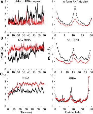
RMSD (left column) and RMSF (right column) time series for the explicit (black) and implicit (red) solvent simulations of the A-form RNA duplex (A), SRL rRNA (B), and tRNA (C). Only the productive trajectories are displayed here after excluding all preequilibration frames. Frames from the first 20 ns of the productive simulations are excluded from RMSF calculation.

Hydrogen bonding is a key factor stabilizing RNA structures and determining the specificity in base pairing. Hence, the numbers of interchain hydrogen bonds are computed throughout both trajectories using the criterion that the acceptor–donor distance is smaller than 3.5 Å and the acceptor–H–donor angle exceeds 140 degrees. The left panel of Fig. 2 A indicates that the number of hydrogen bonds in the implicit solvent system is relatively constant with limited fluctuations. Furthermore, the average number of hydrogen bonds, 28.8, is fairly close to the value (26.5) in the explicit solvent system.

Figure 2.

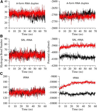
Time series of hydrogen bonds (left column) and electrostatic potentials (right column) for the explicit (black) and implicit (red) solvent simulations of the A-form RNA duplex (A), SRL rRNA (B), and tRNA (C). Only the productive trajectories are displayed here after excluding all preequilibration frames.

Our model is designed to provide a better description of the electrostatics in the implicit solvent. Hence, the electrostatic contributions (ΔG_E) to the free energy are evaluated for both trajectories by summing over two components: the electrostatic potential (E_EL), which is calculated directly using traditional molecular mechanics, and the electrostatic interaction contribution to the solvation energy (E_PB), which is estimated by solving the PB equation. The time dependence of the total electrostatic energy (Fig. 2 A, right panel) is quite similar for the explicit and implicit solvent systems, a similarity supported by their overlapping statistical distributions (−2703 ± 18 and −2714 ± 14 kcal/mol for the explicit and implicit solvent systems, respectively; Table 1). The resemblance is present in the total electrostatic interaction energy and also in the two contributing components E_EL and E_PB.

Table 1.

Electrostatic interactions from the simulations for the three RNA molecules

System		Simulation time (ns)	EEL (kcal/mol)	EPB (kcal/mol)	ΔGE (kcal/mol)	Disparity (%)
RNA duplex	Explicit	70	2200 ± 97	−4903 ± 96	−2703 ± 18	−0.4
	Implicit	70	2250 ± 48	−4964 ± 46	−2714 ± 14
SRL rRNA	Explicit+Mg2+	70	5533 ± 217	−9604 ± 206	−4071 ± 22	4.0
	Implicit+Mg2+	70	5977 ± 85	−9885 ± 79	−3908 ± 21
	Explicit	50	5576 ± 111	−9649 ± 102	4073 ± 21	1.7
	Implicit	50	5663 ± 121	−9665 ± 114	4002 ± 20
tRNA	Explicit+Mg2+	60	33,454 ± 549	−43,906 ± 529	−10,452 ± 38	3.6
	Implicit+Mg2+	60	33,486 ± 407	−43,560 ± 357	−10,074 ± 74
	Explicit	10	33,540 ± 396	−44,019 ± 382	−10,479 ± 31	2.0
	Implicit	10	32,735 ± 364	−43,002 ± 371	−10,266 ± 74

E_EL is the electrostatic interaction calculated according to molecular mechanics (using the AMBER99 force field). E_PB is the electrostatic contribution to the solvation energy and is estimated by solving the PB equation. ΔG_E is the total electrostatic contribution to the system free energy and is therefore computed as the sum of E_EL and E_PB. The disparity is the relative difference of ΔG_E from the implicit solvent system with respect to the corresponding explicit solvent system. Explicit+Mg²⁺ and implicit+Mg²⁺ indicate the presence of explicit Mg²⁺ ions in the explicit and implicit solvent simulations.

The A-form RNA duplex displays an anomalous jump in both RMSD and the number of hydrogen bonds around 36 ns in the explicit solvent simulation (black line in the left panels of Fig. 1 A and Fig. 2 A). The jump in RMSD is mainly caused by bending of the duplex (Fig. S3, A and B), a motion that also substantially increases structural fluctuations (RMSF) of the middle nucleotides (Fig. 1 A, right panel). On the other hand, the abrupt change in the number of hydrogen bonds is induced by the flipping of the terminal cytocines at both ends, which locally disrupts the G–C base pairing (Fig. S3, C and D). Except for these minor differences, the A-form RNA duplex displays similar dynamics in the implicit and explicit solvent simulations, indicating that the implicit solvent model performs as well as the explicit solvent model for this small RNA duplex.

SRL rRNA simulation

SRL rRNA is an indispensable component of the ribosome and plays an important role in the binding and recognition with several elongation factors (e.g., Ef-G and Ef-Tu) involved in protein synthesis (48). Therefore, its mechanism of recognition has been extensively studied both experimentally and computationally (30,49).

SRL rRNA is structurally stable in the implicit solvent simulation, as indicated by the steady RMSD (∼3.3 Å) that follows a rapid rise in the early stage (Fig. 1 B, left panel). In contrast, the RMSD for the explicit solvent simulation is small in the early stage (∼2.2 Å), grows continuously during the simulation, and finally stabilizes at a structural deviation (∼3.2 Å) comparable to that of the implicit solvent simulation at the end of the 70-ns trajectory. Similar patterns of RMSFs (Fig. 1 B, right panel) appear in both simulations, despite the slightly smaller magnitude in the implicit solvent simulation. Particularly, the first three nucleotides at the 5′-end are significantly more flexible in the explicit solvent trajectory, a feature that is less well captured by the implicit solvent simulation. On the other hand, both implicit and explicit solvent simulations exhibit a large positional fluctuation of nucleotide 15, which corresponds to nucleotide 2660 (A2660) in 23S rRNA of Escherichia coli. As the outermost residue in the GAGA tetra-loop, this nucleotide is supposed to be structurally flexible to facilitate its involvement in recognition by the elongation factors as well as in sarcin/ricin binding (48). Our implicit solvent simulation, hence, correctly reflects this structural flexibility and agrees with a previous explicit solvent simulation (49). The Watson–Crick region (helix at the 5′- and 3′-ends) of the SRL rRNA adopts an A-form-like duplex in the crystal structure (30), and the native conformation of this region is well maintained in the implicit solvent simulation (Fig. S4). The stability of SRL rRNA degrades when Mg²⁺ ions are absent in the implicit solvent simulation, as indicated by the remarkably greater RMSD (Fig. S5, left panel). This suggests the necessity of including the explicit divalent ions in our model.

The left panel of Fig. 2 B indicates the presence of nearly identical numbers of intramolecular hydrogen bonds in the implicit (59.5 ± 4.9) and explicit (60.3 ± 5.0) solvent simulations. The resemblance of the two trajectories implies that the base pairs undergo a similar level of rearrangement in the two simulations.

Despite the comparable magnitudes of the RMSD, RMSF, and hydrogen bonds in both classes of simulation, the electrostatic contribution (ΔG_E) to the free energy differs substantially in the two simulations (Fig. 2 B, right panel). The electrostatic contribution of about −4071 kcal/mol to the free energy in the explicit solvent system contrasts with the average of −3908 kcal/mol for the implicit solvent system, an underestimation for this RNA molecule by ∼4% from our model (Table 1). Interestingly, the mismatches between explicit and implicit solvent systems are larger in the individual contributions (E_EL and E_PB in Table 1), but they cancel to some degree in the total ΔG_E.

tRNA simulation

The tRNAs contain 73 to 94 nucleotides and adopt an L-shaped, compact structure. The strong electrostatic repulsion between the portions of the spatially localized phosphate backbone introduces difficulty in accurately simulating tRNAs with an implicit solvent model. The molecules are liable to severely distort if the electrostatics are not correctly described. To our knowledge, no tRNA molecules or comparable nucleic acids have previously been successfully simulated with an implicit solvent model.

The tRNA structure undergoes relatively large conformational changes during the first 20 ns of both the explicit and implicit solvent simulations and then equilibrates gradually (Fig. 1 C, left panel). The RMSD profiles indicate that the structural change is 2–3 Å larger in the implicit solvent simulation. Close inspection, however, suggests that this difference is partially caused by the highly dynamical unpaired 3′-end because the RMSD values drop dramatically when the five unpaired nucleotides at the 3′-end are excluded from the RMSD calculation (Fig. S6). In other words, the main body of the tRNA is structurally stable in the implicit solvent simulation, although the RMSD is ∼1.5 Å higher than that for the explicit solvent simulation. This result represents, as far as we know, the first example of a complex RNA molecule (e.g., tRNA) that has been successfully simulated with a computationally rapid implicit solvent model. The RMSFs calculated from both the implicit and explicit solvent trajectories support the assignment of high structural flexibility to the unpaired 3′-end (Fig. 1 C, right panel). In addition, the overall RMSF pattern for the implicit solvent simulation matches that for the explicit solvent trajectory, despite a minor difference in the dihydrouracil arm (nucleotides 8–14), in which the implicit solvent simulation exhibits slightly larger RMSF values (Fig. 1 C, right panel). In general, the main body of the tRNA is well characterized by our implicit solvent model. In contrast, the tRNA cannot maintain a compact structure when Mg²⁺ ions are absent in our implicit solvent simulation, as reflected by the rapid growth of the RMSD (to ∼10 Å) in a 10-ns simulation (Fig. S5, right panel).

Similar to the smaller systems, the number of intramolecular hydrogen bonds of tRNA in the implicit solvent simulation agrees well with the number derived from the explicit solvent simulation (Fig. 2 C, left panel). On average, both systems have 141 intramolecular hydrogen bonds with similar standard deviations (7.8 and 8.3 for explicit and implicit solvent systems, respectively). Furthermore, the small fluctuations of the number of hydrogen bonds along both trajectories indicate that the overall base-pairing pattern in tRNA is quite stable.

As found in the SRL rRNA simulations, the electrostatic contribution to the free energy is underestimated by 3.6% in magnitude from the implicit solvent simulation of tRNA (Fig. 2 C, right panel; Table 1).

In summary, simulations for the three RNA systems demonstrate that our implicit solvent model can efficiently facilitate the simulation of RNA molecules with different structural complexity. The simulated molecules display comparable structural changes and fluctuations (e.g., RMSD, RMSF, hydrogen bonds, etc.) to the explicit solvent simulations. However, the model underestimates the electrostatic energies by ∼4% when simulating the relatively compact RNA structures (SRL rRNA and tRNA), a flaw that may arise from deficiencies in the model (see Discussion section).

Discussion

Comparison with other implicit solvent models

Although we demonstrate good performance of our implicit solvent model, an objective evaluation of its power for RNA simulations requires comparison of the model with other available implicit solvent models, which overwhelmingly involve GBSA models, of which the GB_HCT model (43,44) has been reported as superior to other GB models in handling nucleic acids (42). Test simulations using the GB_HCT model (in AMBER) satisfactorily describe both the RNA duplex and SRL rRNA as structurally stable, albeit with slightly larger average RMSDs than our model (Table 2). The GB_HCT model, however, fails in simulating tRNA: The overall tertiary topology quickly becomes lost in a 10-ns simulation (as indicated in Table 2 by the average RMSD of 14.8 Å in the last 1 ns of the 10-ns trajectory and in Fig. 3 by the structure of RNA in the last frame). Two other popular GB models, GB_OBC1 (45) and GB_OBC2 (46) in AMBER, are also evaluated for their power in tRNA simulation. Table S2 shows that tRNA fails to maintain its tertiary structure in any of the GB models tested above, either in the presence or in the absence of explicit Mg²⁺ ions (and similar results emerge using the GB_OBC model in NAMD). The last frames of the 10-ns trajectories (Fig. 3) clearly imply that the L-shaped tertiary structure of tRNA is well preserved only from the simulation with our superior implicit solvent model.

Table 2.

Comparison between our model and the GB_HCT model in the simulations of the three RNAs

System	RMSD in the last 1 ns (Å)
	Our model	GBHCT
A-form RNA duplex	1.44 ± 0.12	2.79 ± 0.68
SRL rRNA	3.34 ± 0.13	4.47 ± 0.79
tRNA	5.13 ± 0.16	14.76 ± 0.75

RMSD values of simulated RNA molecules relative to the initial conformations are calculated for structural snapshots in the last 1 ns of the 10-ns simulations using our implicit solvent model and the GB_HCT model. Mg²⁺ ions are present in both implicit solvent simulations.

Figure 3.

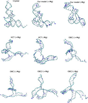
The last frames in 10-ns simulations of tRNA using our model as well as from the GB_HCT, GB_OBC1, and GB_OBC2 models, with (+Mg) or without Mg²⁺ (−Mg) ions included. Consistent with Table S2, the simulations using our model exhibit the tertiary structure of tRNA as intact when Mg²⁺ ions are present, but as partially distorted when Mg²⁺ ions are absent. In contrast, the tertiary topology is nearly completely disrupted in all other implicit solvent models tested, independent of whether or not Mg²⁺ ions are included in the simulation system.

Possible future improvements

We propose a novel, to our knowledge, implicit solvent model to simulate the structure and dynamics of RNA molecules by combining the LD model and the PB equation. Despite its acceptable performance in simulating large RNA molecules, which to our knowledge is not feasible using other available models, the model still possesses deficiencies that should be overcome in the future.

First, the binding and coordination of Mg²⁺ ions are incorrectly represented, although these ions are absolutely necessary in our model (as shown above in the implicit solvent simulations of SRL rRNA and tRNA when Mg²⁺ ions are absent). In the real binding process, Mg²⁺ frequently loses most of the water molecules in its first hydration layer and closely coordinates with the electronegative oxygen and nitrogen atoms in RNA. Therefore, any inaccuracy in estimating the desolvation energy of Mg²⁺ ions may negatively impact the description of the thermodynamics of RNA molecules. Unfortunately, despite the consideration of the solvation energy for all RNA atoms, the desolvation of Mg²⁺ ions is neglected in our present implicit solvent model because we have not found a better way to estimate the electrostatics of these ions than the current PB-based model, which has intrinsic flaws in handling the divalent ions in the absence of explicit solvent. Without the desolvation penalty, Mg²⁺ ions prefer more intimate interaction with the RNA molecules, as demonstrated in Fig. S7, in which the RNA atoms are counted as coordinated when they are located within 2.4 Å (see Petrov et al. (50)) of any of the seven Mg²⁺ ions in the simulation of tRNA. The bias for overcoordination frequently disrupts the RNA structures locally in the implicit solvent simulations (Fig. S8). More important, the local disruption of RNA structures would further affect the electrostatic calculations. In contrast to the A-form RNA duplex, systems with explicit Mg²⁺ ions (SRL rRNA and tRNA) have a ∼4% disparity in the total electrostatics (Table 1), which implies a possible side effect of the nonideal treatment of Mg²⁺. To quantify the effect of Mg²⁺ ions on the underestimation of electrostatics, implicit and explicit solvent simulations for SRL rRNA (50 ns) and tRNA (10 ns) are performed without the Mg²⁺ ions. The electrostatic energies now agree better (to disparities of ∼1.7% and 2.0%, respectively, in Table 1), suggesting that the implicit solvent model described here can be further improved by including an improved description of divalent ions.

Second, our implicit solvent model is derived by combining the LD model and the PB equation for a point charge. Ideally, both the dielectric function and the electrical displacement should be determined by multiple rounds of iterative calculations using Eq. 6 and Eq. 8. The present work approximates the numerical solution of Eq. 6 by a fitting function (Eq. 7), and the iterative calculation is truncated at the first iteration to derive a simple analytical formula for the dielectric function. Moreover, the real RNA molecules contain numerous charged atoms rather than one point charge, and the dielectric function should not be spherically symmetric in such a complex system. Therefore, the dielectric function should be derived following the iterative approach and considering more information about the target (e.g., the shape and charge distribution of the molecule).

Finally, the model is currently implemented in STINKER, a simulation package without parallelization, which impairs the efficiency of the program. In particular, a benchmark test for implicit solvent simulation of tRNA on a DELL workstation (2.67GHz CPU, Intel core i7) suggests a performance of ∼0.8 ns/day per core processor, which is 6 times faster than the explicit solvent simulation using NAMD (0.125 ns/day) when one CPU processor is used. However, the NAMD simulations can be accelerated by 16 times (to 2 ns/day) when 24 Intel Xeon 2.67GHz processers are used. In the future, our model should be incorporated into a well-parallelized program to facilitate faster RNA simulations.

References

- 1.McDowell S.E., Spacková N., Walter N.G. Molecular dynamics simulations of RNA: an in silico single molecule approach. Biopolymers. 2007;85:169–184. doi: 10.1002/bip.20620. [DOI] [PMC free article] [PubMed] [Google Scholar]
- 2.Khalili-Araghi F., Gumbart J., Schulten K. Molecular dynamics simulations of membrane channels and transporters. Curr. Opin. Struct. Biol. 2009;19:128–137. doi: 10.1016/j.sbi.2009.02.011. [DOI] [PMC free article] [PubMed] [Google Scholar]
- 3.Klepeis J.L., Lindorff-Larsen K., Shaw D.E. Long-timescale molecular dynamics simulations of protein structure and function. Curr. Opin. Struct. Biol. 2009;19:120–127. doi: 10.1016/j.sbi.2009.03.004. [DOI] [PubMed] [Google Scholar]
- 4.Mackerell A.D., Jr., Nilsson L. Molecular dynamics simulations of nucleic acid-protein complexes. Curr. Opin. Struct. Biol. 2008;18:194–199. doi: 10.1016/j.sbi.2007.12.012. [DOI] [PMC free article] [PubMed] [Google Scholar]
- 5.Hashem Y., Auffinger P. A short guide for molecular dynamics simulations of RNA systems. Methods. 2009;47:187–197. doi: 10.1016/j.ymeth.2008.09.020. [DOI] [PubMed] [Google Scholar]
- 6.Li W., Frank J. Transfer RNA in the hybrid P/E state: correlating molecular dynamics simulations with cryo-EM data. Proc. Natl. Acad. Sci. USA. 2007;104:16540–16545. doi: 10.1073/pnas.0708094104. [DOI] [PMC free article] [PubMed] [Google Scholar]
- 7.Aleksandrov A., Simonson T. Molecular dynamics simulations of the 30S ribosomal subunit reveal a preferred tetracycline binding site. J. Am. Chem. Soc. 2008;130:1114–1115. doi: 10.1021/ja0741933. [DOI] [PubMed] [Google Scholar]
- 8.Tajkhorshid E., Nollert P., Schulten K. Control of the selectivity of the aquaporin water channel family by global orientational tuning. Science. 2002;296:525–530. doi: 10.1126/science.1067778. [DOI] [PubMed] [Google Scholar]
- 9.Cramer C.J., Truhlar D.G. Implicit solvation models: equilibria, structure, spectra, and dynamics. Chem. Rev. 1999;99:2161–2200. doi: 10.1021/cr960149m. [DOI] [PubMed] [Google Scholar]
- 10.Still W.C., Tempczyk A., Hendrickson T. Semianalytical treatment of solvation for molecular mechanics and dynamics. J. Am. Chem. Soc. 1990;112:6127–6129. [Google Scholar]
- 11.Ho B.K., Dill K.A. Folding very short peptides using molecular dynamics. PLOS Comput. Biol. 2006;2:e27. doi: 10.1371/journal.pcbi.0020027. [DOI] [PMC free article] [PubMed] [Google Scholar]
- 12.Onufriev A., Case D.A., Bashford D. Effective Born radii in the generalized Born approximation: the importance of being perfect. J. Comput. Chem. 2002;23:1297–1304. doi: 10.1002/jcc.10126. [DOI] [PubMed] [Google Scholar]
- 13.Im W., Feig M., Brooks C.L., 3rd An implicit membrane generalized born theory for the study of structure, stability, and interactions of membrane proteins. Biophys. J. 2003;85:2900–2918. doi: 10.1016/S0006-3495(03)74712-2. [DOI] [PMC free article] [PubMed] [Google Scholar]
- 14.Xu Z., Cheng X., Yang H. Treecode-based generalized Born method. J. Chem. Phys. 2011;134:064107. doi: 10.1063/1.3552945. [DOI] [PubMed] [Google Scholar]
- 15.Wang Y., Wallace J.A., Shen J.K. Molecular dynamics simulations of ionic and nonionic surfactant micelles with a generalized Born implicit-solvent model. J. Comput. Chem. 2011;32:2348–2358. doi: 10.1002/jcc.21813. [DOI] [PubMed] [Google Scholar]
- 16.Tsui V., Case D.A. Molecular dynamics simulations of nucleic acids with a generalized Born solvation model. J. Am. Chem. Soc. 2000;122:2489–2498. [Google Scholar]
- 17.Tsui V., Case D.A. Calculations of the absolute free energies of binding between RNA and metal ions using molecular dynamics simulations and continuum electrostatics. J. Phys. Chem. B. 2001;105:11314–11325. [Google Scholar]
- 18.Sarzynska J., Nilsson L., Kulinski T. Effects of base substitutions in an RNA hairpin from molecular dynamics and free energy simulations. Biophys. J. 2003;85:3445–3459. doi: 10.1016/S0006-3495(03)74766-3. [DOI] [PMC free article] [PubMed] [Google Scholar]
- 19.Chocholousová J., Feig M. Implicit solvent simulations of DNA and DNA-protein complexes: agreement with explicit solvent vs experiment. J. Phys. Chem. B. 2006;110:17240–17251. doi: 10.1021/jp0627675. [DOI] [PubMed] [Google Scholar]
- 20.Prabhu N.V., Panda M., Sharp K.A. Explicit ion, implicit water solvation for molecular dynamics of nucleic acids and highly charged molecules. J. Comput. Chem. 2008;29:1113–1130. doi: 10.1002/jcc.20874. [DOI] [PubMed] [Google Scholar]
- 21.Gaillard T., Case D.A. Evaluation of DNA force fields in implicit solvation. J. Chem. Theory Comput. 2011;7:3181–3198. doi: 10.1021/ct200384r. [DOI] [PMC free article] [PubMed] [Google Scholar]
- 22.Gavryushov S. Dielectric saturation of the ion hydration shell and interaction between two double helices of DNA in mono- and multivalent electrolyte solutions: foundations of the epsilon-modified Poisson-Boltzmann theory. J. Phys. Chem. B. 2007;111:5264–5276. doi: 10.1021/jp067120z. [DOI] [PubMed] [Google Scholar]
- 23.Gong H., Hocky G.M., Freed K.F. Influence of nonlinear electrostatics on transfer energies between liquid phases: charge burial is far less expensive than Born model. Proc. Natl. Acad. Sci. USA. 2008;105:11146–11151. doi: 10.1073/pnas.0804506105. [DOI] [PMC free article] [PubMed] [Google Scholar]
- 24.Gong H., Freed K.F. Langevin-Debye model for nonlinear electrostatic screening of solvated ions. Phys. Rev. Lett. 2009;102:057603. doi: 10.1103/PhysRevLett.102.057603. [DOI] [PubMed] [Google Scholar]
- 25.Debye P., Pauling L. The inter-ionic attraction theory of ionized solutes. IV. The influence of variation of dielectric constant on the limiting law for small concentrations. J. Am. Chem. Soc. 1925;47:2129–2134. [Google Scholar]
- 26.Onsager L. Electric moments of molecules in liquids. J. Am. Chem. Soc. 1936;58:1486–1493. [Google Scholar]
- 27.Kirkwood J.G. The dielectric polarization of polar liquids. J. Chem. Phys. 1939;7:911–919. [Google Scholar]
- 28.Baker N.A., Sept D., McCammon J.A. Electrostatics of nanosystems: application to microtubules and the ribosome. Proc. Natl. Acad. Sci. USA. 2001;98:10037–10041. doi: 10.1073/pnas.181342398. [DOI] [PMC free article] [PubMed] [Google Scholar]
- 29.Miller B.R., McGee T.D., Roitberg A.E. MMPBSA.py: an efficient program for end-state free energy calculations. J. Chem. Theory Comput. 2012;8:3314–3321. doi: 10.1021/ct300418h. [DOI] [PubMed] [Google Scholar]
- 30.Correll C.C., Munishkin A., Steitz T.A. Crystal structure of the ribosomal RNA domain essential for binding elongation factors. Proc. Natl. Acad. Sci. USA. 1998;95:13436–13441. doi: 10.1073/pnas.95.23.13436. [DOI] [PMC free article] [PubMed] [Google Scholar]
- 31.Comarmond M.B., Giege R., Fischer J. Three-dimensional structure of yeast tRNAAsp. I. Structure determination. Acta Crystallogr. B. 1986;42:272–280. [Google Scholar]
- 32.Baird N.J., Gong H., Sosnick T.R. Extended structures in RNA folding intermediates are due to nonnative interactions rather than electrostatic repulsion. J. Mol. Biol. 2010;397:1298–1306. doi: 10.1016/j.jmb.2010.02.025. [DOI] [PMC free article] [PubMed] [Google Scholar]
- 33.Grossfield A., Ren P., Ponder J.W. Ion solvation thermodynamics from simulation with a polarizable force field. J. Am. Chem. Soc. 2003;125:15671–15682. doi: 10.1021/ja037005r. [DOI] [PubMed] [Google Scholar]
- 34.Shen M.Y., Freed K.F. All-atom fast protein folding simulations: the villin headpiece. Proteins. 2002;49:439–445. doi: 10.1002/prot.10230. [DOI] [PubMed] [Google Scholar]
- 35.Jha A.K., Freed K.F. Solvation effect on conformations of 1,2:dimethoxyethane: charge-dependent nonlinear response in implicit solvent models. J. Chem. Phys. 2008;128:034501. doi: 10.1063/1.2815764. [DOI] [PMC free article] [PubMed] [Google Scholar]
- 36.Cornell W.D., Cieplak P., Kollman P.A. A second generation force field for the simulation of proteins, nucleic acids, and organic molecules. J. Am. Chem. Soc. 1995;117:5179–5197. [Google Scholar]
- 37.Ooi T., Oobatake M., Scheraga H.A. Accessible surface areas as a measure of the thermodynamic parameters of hydration of peptides. Proc. Natl. Acad. Sci. USA. 1987;84:3086–3090. doi: 10.1073/pnas.84.10.3086. [DOI] [PMC free article] [PubMed] [Google Scholar]
- 38.Kelly C.P., Cramer C.J., Truhlar D.G. SM6: a density functional theory continuum solvation model for calculating aqueous solvation free energies of neutrals, ions, and solute-water clusters. J. Chem. Theory Comput. 2005;1:1133–1152. doi: 10.1021/ct050164b. [DOI] [PubMed] [Google Scholar]
- 39.Forti F., Barril X., Orozco M. Extension of the MST continuum solvation model to the RM1 semiempirical Hamiltonian. J. Comput. Chem. 2008;29:578–587. doi: 10.1002/jcc.20814. [DOI] [PubMed] [Google Scholar]
- 40.Phillips J.C., Braun R., Schulten K. Scalable molecular dynamics with NAMD. J. Comput. Chem. 2005;26:1781–1802. doi: 10.1002/jcc.20289. [DOI] [PMC free article] [PubMed] [Google Scholar]
- 41.Case D.A., Darden T.A., Kollman P.A. University of San Francisco; San Francisco, CA: 2012. AMBER 12. [Google Scholar]
- 42.Gong Z., Xiao Y., Xiao Y. RNA stability under different combinations of amber force fields and solvation models. J. Biomol. Struct. Dyn. 2010;28:431–441. doi: 10.1080/07391102.2010.10507372. [DOI] [PubMed] [Google Scholar]
- 43.Hawkins G.D., Cramer C.J., Truhlar D.G. Pairwise solute descreening of solute charges from a dielectric medium. Chem. Phys. Lett. 1995;246:122–129. [Google Scholar]
- 44.Hawkins G.D., Cramer C.J., Truhlar D.G. Parametrized models of aqueous free energies of solvation based on pairwise descreening of solute atomic charges from a dielectric medium. J. Phys. Chem. 1996;100:19824–19839. [Google Scholar]
- 45.Onufriev A., Bashford D., Case D.A. Modification of the generalized Born model suitable for macromolecules. J. Phys. Chem. B. 2000;104:3712–3720. [Google Scholar]
- 46.Onufriev A., Bashford D., Case D.A. Exploring protein native states and large-scale conformational changes with a modified generalized born model. Proteins. 2004;55:383–394. doi: 10.1002/prot.20033. [DOI] [PubMed] [Google Scholar]
- 47.Humphrey W., Dalke A., Schulten K. VMD: visual molecular dynamics. J. Mol. Graph. 1996;14:33–38. doi: 10.1016/0263-7855(96)00018-5. 27–38. [DOI] [PubMed] [Google Scholar]
- 48.Moazed D., Robertson J.M., Noller H.F. Interaction of elongation factors EF-G and EF-Tu with a conserved loop in 23S RNA. Nature. 1988;334:362–364. doi: 10.1038/334362a0. [DOI] [PubMed] [Google Scholar]
- 49.Spacková N., Sponer J. Molecular dynamics simulations of sarcin-ricin rRNA motif. Nucleic Acids Res. 2006;34:697–708. doi: 10.1093/nar/gkj470. [DOI] [PMC free article] [PubMed] [Google Scholar]
- 50.Petrov A.S., Bowman J.C., Williams L.D. Bidentate RNA-magnesium clamps: on the origin of the special role of magnesium in RNA folding. RNA. 2011;17:291–297. doi: 10.1261/rna.2390311. [DOI] [PMC free article] [PubMed] [Google Scholar]
Associated Data
This section collects any data citations, data availability statements, or supplementary materials included in this article.