A computational neural model of orientation detection based on multiple guesses: comparison of geometrical and algebraic models

Abstract

The implementation of Hubel-Wiesel hypothesis that orientation selectivity of a simple cell is based on ordered arrangement of its afferent cells has some difficulties. It requires the receptive fields (RFs) of those ganglion cells (GCs) and LGN cells to be similar in size and sub-structure and highly arranged in a perfect order. It also requires an adequate number of regularly distributed simple cells to match ubiquitous edges. However, the anatomical and electrophysiological evidence is not strong enough to support this geometry-based model. These strict regularities also make the model very uneconomical in both evolution and neural computation. We propose a new neural model based on an algebraic method to estimate orientations. This approach synthesizes the guesses made by multiple GCs or LGN cells and calculates local orientation information subject to a group of constraints. This algebraic model need not obey the constraints of Hubel-Wiesel hypothesis, and is easily implemented with a neural network. By using the idea of a satisfiability problem with constraints, we also prove that the precision and efficiency of this model are mathematically practicable. The proposed model makes clear several major questions which Hubel-Wiesel model does not account for. Image-rebuilding experiments are conducted to check whether this model misses any important boundary in the visual field because of the estimation strategy. This study is significant in terms of explaining the neural mechanism of orientation detection, and finding the circuit structure and computational route in neural networks. For engineering applications, our model can be used in orientation detection and as a simulation platform for cell-to-cell communications to develop bio-inspired eye chips.

Introduction

Orientation detection importance in scene perception

From a semantic perspective, orientations are a type of geometrical features at the intermediate level, between the lower pixel level and the higher shape level. Almost all images, from natural scenes to man-made environments, contain a rich amount of information about orientations. Besides their universality, orientations always provide essential structural clues to form the semantics of an image. Also, as a type of feature, orientations are the results of integration, and begin to have semantic attributes. Itti and Koch (2001) proposed a saliency map model for visual search that is underlain by detected orientations and lines as key features. Orientation detection is task-independent and indispensable to image understanding. These aspects make orientations one of the most fundamental and general kinds of features for image representation. Comparing mammal vision and machine vision, the former is not as powerful as the latter when distinguishing minute differences. Human eyes are absolutely imprecise compared with a laser rangefinder, sonar or a light meter. The real and dominant advantage of human vision is its ability to quickly grasp the overall meaning of image. There have been many researches on the integrations of oriented edges for object recognition related tasks (Sakai and Nishimura 2006; Craft et al. 2007; Mihalas et al. 2011; Wagatsuma et al. 2008; Sajda and Baek 2004).

Orientation detection problems in traditional digital image processing

Many studies of orientation detection have been conducted in traditional digital image processing. Generally, the process can be realized in two steps: the first step is edge detection, the pixels with large gradient values of gray-level are marked as edges (all of the pixels are merely discrete points); the second step is line detection, collinear edges are aggregated and then the line equations which best fit these points are found. However, these methods are normally based on combinations, searches and optimizations. There are several drawbacks including high algorithm complexity, sensitivity to parameter selection, few interventions with high level knowledge.

Also, problems such as how to combine the results of orientation detection processes, how to produce a high level structure description for the image content and how to formalize these processes are extremely difficult successive operations. Line detection algorithms cannot generate an abstract and spatial organization for the detection results. In other words, the generation of an explicit symbolic representation to reflect the spatial correlation of the lines is not the object of line detection. Therefore, traditional representation of the orientations using a concise mathematical vector is not necessarily appropriate for the follow-up tasks such as searching, combination and optimization, despite its low memory cost.

Orientation detection in the brain

According to the neurobiological studies on the neural mechanism of vision, a multi-level network with a feedback control can achieve orientation detection instantaneously, and the results are eventually stored in the primary visual cortex. The GCs and the LGN cells play important roles in orientation detection. These two level cells serve as inevitable links between the levels of stimuli and the level of meaning. The concentric RFs of GCs and LGN cells are responsible for the primary integrations of physical stimuli, and all the subsequent visual tasks stem from the representation produced by these cells. It is found that the orientation preference maps caused by correlated visual stimuli show geometrical regularities similar to those observed in natural images (Tang et al. 2011). Hubel and Wiesel, two Nobel Prize laureates, proposed a famous hypothesis about the construction of simple cells’ RFs. This theory has become the basic model for the visual cortex to perceive and represent orientations in the outside world.

Potential difficulties with Hubel-Wiesel hypothesis

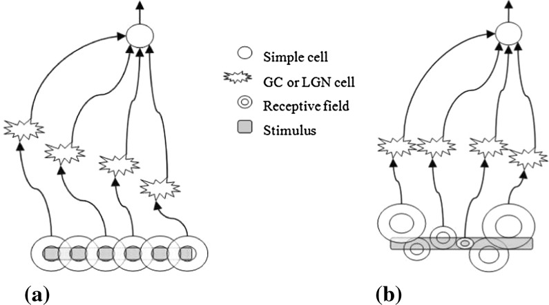
Hubel and Wiesels hierarchical model of simple cell RFs assumes that a V1 simple cell receives inputs from several LGN cells. The ultimately equivalent RFs of these LGN cells in the visual field are lined up in a regular band. This enables the simple cell’s selectivity to the orientation of a light bar. From a computational perspective, this kind of simple cell model with a geometric regularity in its RF pays no cost for the calculation. However, the correctness of this geometric-based model has not yet been proved. Anatomical studies have shown that a simple cell truly receives the outputs of multiple lined-up LGN cells. However, this does not sufficiently prove that the achievement of orientation can be attributed only to the fact that several LGN cells’ RFs are covered by the identical stimulus patterns and then produce the same responses.

The assumptions behind this idea are fairly idealized. (1) The RFs of the LGN cells and the GCs are required to be arranged in a very orderly manner in the visual field. Specifically, the center regions of the concentric RFs should be arranged collinearly. (2) The size of each RF is required to be uniform. (3) On-cell and off-cell structures are required to be arranged in an orderly fashion. (4) The light stimulus bar should be moderate in width and cover several RFs in almost the same fashion. (5) In order to precisely detect all orientations with different slopes at different positions, the distribution of all cells and their RFs is therefore required to be highly ordered. These initialization constraints seem to be much idealized for a biological system, and make it difficult to be generated or evolved. Alonso et al. (2001) has reported these factors’ negative effects on orientation selectivity acquisition.

Meanwhile, doubts have been expressed about this classical hypothesis (Sompolinsky and Shapley 1997; Wielaard et al. 2001; Ferster and Miller 2000). This hypothesis has been considered insufficient in its original state (Lauritzen and Miller 2003). Other models describing the mechanism of simple cells have been proposed. Some of these models studied new structures of the RFs (Hansen et al. 2000; Kara et al. 2002; Lee et al. 2000; Liu et al. 2010), while others improved the theories of contrast-invariant orientation tuning (Troyer et al. 2002). Some re-examined the formation of orientation selectivity of the simple cells (Bhaumik and Mathur 2003; Gardner et al. 1999; Wielaard et al. 2001). Yang et al. (2011) developed a feed-forward hierarchy network constructing the circuitry for orientation selectivity of the visual cortex. Alexander and Van Leeuwen (2010) introduced a hypothesis about the organization of V1’s contextual response.

Cai et al. (2004) and Tao et al. (2004) studied the issues such as how the function of the simple cell emerges in the primary visual cortex and how to design a dynamics model. Smyth et al. (2003), Stephen and Jack (2005) and Willmore et al. (2000) discussed whether and how the simple cells reflect the statistical features of natural images. Wallis (2001) improved a linear filter commonly used to model the simple cell. Rich et al. (2001) studied the spatio-temporal effect of cAMP signals in the simple cell. McAdams and Reid (2005) studied how the response of the simple cell is influenced by attenuation. Norheim et al. (2012) proposed a minimal mechanistic model for LGN relay ON cells including feedforward excitation and inhibition from retinal ON cells and excitatory and inhibitory feedback from cortical ON and OFF cells. However, these previous researches have produced few systematic conclusions for the computational essence of the hierarchical RF-group. We have thus continued to speculate that there may be another type of computational strategy possible under the same local neural connection.

A new model approach

Because the implementation of the standard model is difficult, simple cells may use some other method to detect orientation. The standard model emphasizes a highly ordered distribution of the GCs and LGN cells. This might hide some serious problems, such as an over-crowded arrangement and the inconsistency when sharing a cell and blind spots for detection. We therefore think that such a strict arrangement is not necessary as long as (1) single GCs or LGN cell can recognize the edge falling in their RFs (2) the simple cell can synthetically analyze the outputs from multiple lower LGN cells. Their behaviors are similar to those of a board of directors making a decision collectively, so the final determination must be acceptable for every director. In this case, even randomly-distributed GCs and LGN cells can also work, and this kind of distribution can greatly benefit the generation of the cell array because several strong constraints can be ignored.

Our idea is that a simple cell uses multiple GCs or LGN cells’ nonlinear responses to a light contrast, and reconstructs an internal and subjective orientation to approach an outside edge using constraint satisfaction and group decision. In other words, the difference between this new hypothesis and the classical one is that it is an algebraic model rather than a geometric model. Our brain responds to outside stimuli and produces reasonable explanations for them. This indicates a philosophical fact: what we see is not reality but is only what we sense. It is an image or a virtual reality, i.e. a result rebuilt by our brain. This inner image is called a mental image, and it can be manipulated by the neural system.

The results detected by GCs and LGN cells provide all the data needed for subsequent visual cortex processing. None of the complicated face, object or handwriting recognition processes can be independent of those data (Delorme and Thorpe 2001; Fukushima 2010; Kang and Lee 2002), and therefore considerable attention has been devoted to the studies of the mechanisms of GCs and LGN cells (Hennig and Funke 2001; Niu and Yuan 2007). Gong et al. (2010) discussed the relationship between spike timing correlation and pattern correlation is of GCs. Jing et al. (2010) studied visual pattern recognition based on spatio-temporal patterns of GCs’ activities.

As a special case of the Gabor function, the difference of Gaussian (DOG) function is a concise and reliable model, and its numerical form is also suitable for parallel computing. DOG has also been proved to provide an accurate explanation of the concentric RFs (Gomes 2002; Miikkulainen et al. 2005). The DOG function is widely used to model RFs in the retina (Miikkulainen et al. 2005; Watson and Ahumada 1989), and as a type of filter to detect contour features (Grigorescu et al. 2004; Kolesnik et al. 2002; Long and Li 2008; McKinstry and Guest 2001; Niu and Yuan 2007; Serre et al. 2007). DOG has also been used to join an implanted microchip and the neural tissue (Morillasa et al. 2007), because it can stimulate GCs’ or LGN cells’ responses, and the output signal of the microchip can be explained and accepted by the neural tissue. Einevoll and Plesser (2011) proposed an extended DOG model incorporating cortical feedback for LGN cells.

In view of the benefits of the DOG model in simulating cell response well, we use it to model the concentric RFs at the bottom layer of our system. The innovations in our work are as follows:

1. LGN cells are no longer required to be arranged linearly in the simple cell’s RF. In the photoreceptor layer, the equivalent concentric RFs of the LGN cells are not required to share the same axis. Also, the sizes of these RFs do not need to be unique.

2. This system makes heavy use of the response curve of a GC or LGN cell, and emphasizes even a small variance in the output signal, i.e. it carefully distinguishes the meanings of the different positions on this curve.

3. This system improves the way in which the simple cell recognizes orientations. The conventional method, which simply counts whether all LGN cells in the simple cell’s RF are activated, was abandoned. Instead, the responses of the different LGN cells are used as parameters in an instantaneous solution of a constraint satisfaction problem.

4. Considering that a limited and localized investigation could not reflect the validity of this computational mechanism, we establish a large-scale simple cell layer to represent each possible orientation occurring in the visual field. The balance between the functional requirements and the hardware complexity is also considered.

5. We establish a mathematical model accounting for how a simple cell approaches the orientation process by means of synthesizing multiple localized and scattered guesses. A mathematical test is also conducted to show the precision that this optimization method can achieve, and the error estimation is also considered.

Fig. 1 shows the mechanism of the Hubel-Wiesel model (a) and that of our model (b). This paper puts forward a new theoretical hypothesis, and attempts to make clear several questions which Hubel-Wiesel model does not account for. The novelty of this paper is the proposed explanation of the working mechanism in the Hubel-Wiesel model, and the validity of the explanation is verified by the experiments.

Fig. 1.

The differences between the two mechanisms. a A geometric hyopothesis. Logical calculation: Simple_cell_active. b An algebric optimization:

Single Ganglion-cell modeling

The traditional DOG model

Conceptually, Rodieck (1965) introduced the DOG model to mathematically describe the RF of a GC. This model has proved successful in simulating the responses of major types of GCs to stimuli (such as spot and bar stimuli, grating drifting). The DOG model is a pair of overlapping circularly-symmetric Gaussians (Fig. 2):

1

where δ_c and δ_s are the standard deviations of the central and surrounding Gaussians respectively, and α _c and α _s are the peak sensitivities. The attractiveness of the DOG model is the precision, simplicity and well-formed shape, which benefits the simulations and mathematical analyses greatly. It is therefore used to calculate the responses of GCs to stimuli in our approach.

Fig. 2.

Gaussian function and DOG model. a Center and surround gaussians. b DOG model. c 3D immage of DOG

Using DOG model in a new way

The classical DOG model itself is not new, but we apply it in a new way. In our system, a cell with a DOG-shaped RF acts as a localized multi-valued decision maker.

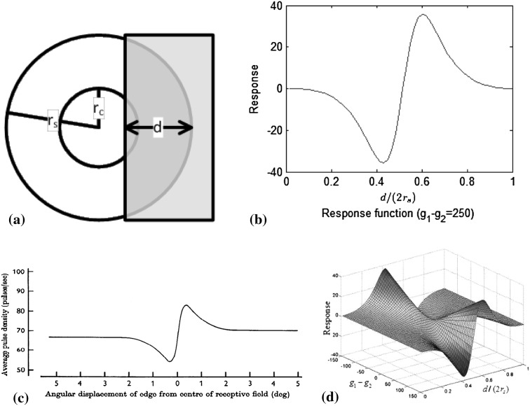
Suppose that there is a sufficiently large stimulus of grayness g₁ that covers part of an RF. The grayness of the background is g₂. This causes an edge between the stimulus and the background. In Fig. 3a, the area of the RF is S, and the sub-area covered by the stimulus is A. The response R of the GC or LGN cell to the stimulus can be calculated as follows:

2

Fig. 3.

A GC responding to stimuli in its RF. a The shadow widens horizontally over an RF. b A GC’s response with respect to the covrage pattern is a function of ratio . c Response of an on-center GC to a contrast edge (Enroth-Cugell and Robson 1966. d The response surface with respect to )

If the stimulus widens horizontally and continuously over the RF, the percentage of the RF that is covered and R will change. Given the values of g₁ and g₂ (for example, g₁ = 251 and g₂ = 1) and a distance d (Fig. 3a), the response R is a function of the ratio (Fig. 3b). This response curve is very similar to the results of biological experiments (Fig. 3c). This proves that the use of the DOG model for stimulation is feasible. Also, by varying the values of g₁, g₂, and d, a three-dimensional surface where g₁ − g₂ is the third variable can be plotted (Fig. 3d). The grayness difference is chosen as a variable to emphasize the fact that a boundary (i.e. an orientation) is the natural result of two neighboring areas of different gray-levels or colors. The most valuable use of this curved surface is to decide on the varying scope of a variable, given the values of the other two variables.

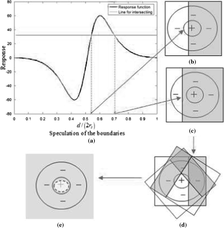
Using the response surface, a cell could roughly judge the approximate position of an edge crossing its RF. We now consider how this is achieved by a single GC or LGN cell. First, when a shadow is being projected onto the RF of a cell, the response R₀ is calculated by the method mentioned above. The curved surface of that cell is then cut vertically along the axis of d/2r_s, and produces a response curve according to the exact grayness difference between the two sides of that shadow. This curve can be expressed as a function R = f(d/2r_s). By cutting the curve using a horizontal line R = R₀, two intersections can normally be obtained (Fig. 4a). Let β_i, i = 1, 2 be the x − coordinates of the two intersections, and each of them may correspond to a possible position at which there is a boundary crossing the RF (Fig. 4b, c). The distance r between the center of RF and the boundary is expressed as:

3

Fig. 4.

The procedures of generating a speculation: a usually, there are two intersections generated by the response R₀. b, c are two possible shadow patterns corresponding to the response given in (a). d Multiple possibilities with different orientations are shown producing the same response. e The common part of all possibilities is a circle, and every one of its tangent lines is a candidate shadow boundary

We consider that the boundary orientation may be arbitrary, i.e. any boundary with the same r can be a valid candidate (Fig. 4d). Therefore, the boundary prediction made by this RF is a concentric circle of radius r of the RF. This circle is a tangent to all the candidate boundaries (Fig. 4e). Two particular details must be considered carefully here: (1) when the response R is close to zero, three possible intersections are obtained (β ₁ = 0, β ₂ = 0.5, and β ₃ = 1). In this case, the RF will not to be used to calculate the boundary. (2) The smaller of the two possible radii is generally chosen to avoid prediction mistakes. Later, we will show that if the correct prediction happens to be the larger radius, the lost area will be compensated by the predictions of other RFs nearby.

Simple cell drawing on collective junior cells

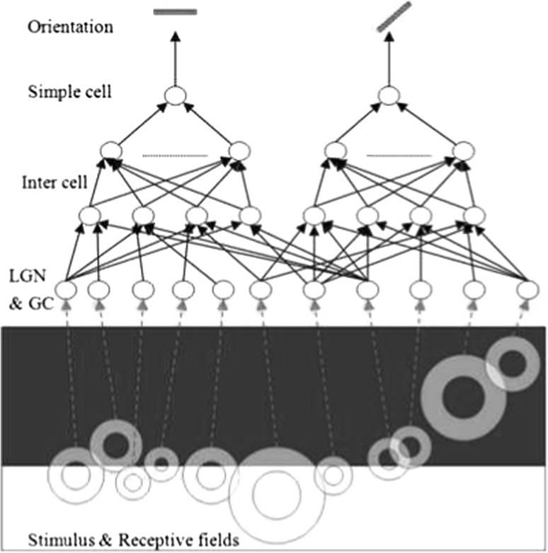
In the previous section, with regard to the boundary of a shadow, it has been shown that what a single GC or LGN cell can judgeis no more than a tangent line. There are infinitely many lines of this kind, and all of them are short and localized in their spatial position. Luckily, there are many cells in the RF of a simple cell, and the compound visual field composed of all these cells has a very limited area. This means that the stimuli that the cells received are all very probably the same segment of a boundary. Therefore, after each inferior cell produces its own speculation, a superior cell seeks for a union guess subject to all the local speculations and is scale-extended. If the speculation produced by a GC or LGN cell is regarded as a set of possible boundaries with different positions and slopes, then the union guess made by a superior cell is the conjunction of these small sets. The scope of this conjunction will reduce dramatically, i.e. the union guess merely includes a few possibilities that can satisfy every cell’s constraint. In other words, a common boundary or several similar boundaries may be found. This reveals a rational method used in a simple cell to determine the position and the slope of a boundary, because it can be done in a manner of parallel distributed processing. This determination process is like voting. A simple cell collects all the clues from its junior cells and synthesizes them for a final determination. To manifest this kind of feasibility, a computational model is designed in this paper to carry out this guess-making task. Figure 5 shows the hierarchical neural network used to calculate the orientation value. This network is composed of multiple back propagation (BP) sub-nets, and the neural connections of each sub-net are strictly localized. Each sub-net simulates a simple cell and its junior cells to implement a collective voting process. The experimental results shown later will prove that this kind of assembly network is sufficient for the implementation of the new mechanism. We choose the traditional BP because it is mature, and its structure and its algorithm is simple and sound. More importantly, if a plain neural network is able to implement a collective voting function, then this function can be easily implemented in the visual cortex since a hypercolumn includes six layers of cells and complicated connections.

Fig. 5.

A neural network model for orientation detection

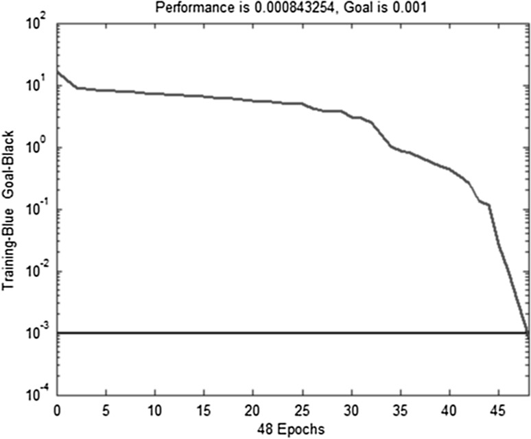
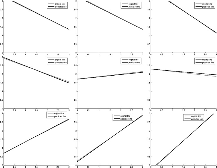
In this paper, an experiment based on the BP Toolkit in Matlab is designed to train and test the network shown in Fig. 5. Given the parameters and the coordinates, eight RFs are distributed over a small region. A set of shadows is also present in this region, and their boundaries swing in at an angle of 20° in total. The orientation difference between two adjacent boundaries is 0.5°, and thus the total number of boundaries is 40. Also, boundaries are expressed as y = ax + b, where x and y are variables, and a and b are parameters. For each shadow stimulus, the eight RFs generate their circular guesses to format an 8 × 1 vector as the input of the network, and the two parameters of this boundary constitute the corresponding output vector of the network. This vector-pair composes a training sample. By repeating this process, a training set can be generated. This training set and the BP algorithm are then used to train the network. The performance of the training process is shown in Fig. 6. It can be seen that the ability to detect orientations can be learned quickly, through no more than a few dozen epochs. Afterwards, some test lines are randomly chosen to format the input vectors, and the corresponding output of this trained network is obtained. After that, we compare the rebuilt lines with the original ones. The results shown in Fig. 7 indicate that this network is precise for boundary detection. This experiment proves that if there are natural boundaries in the scene activating the neural system, then a neural network to detect them could be formed very rapidly.

Fig. 6.

In Matlab BP toolkit, only 48 epochs are used to reduce the error to 0.001

Fig. 7.

Comparisons between the actual boundaries and the detected lines. The contrast stimuli with boundaries are generated in the x − y plane

The mathematical nature of ensemble fitting

Numeric method

Our problem here is to find a common tangent line y = ax + b for a group of circles centered at . If the line does not exist, we seek the line that minimizes . The problem now becomes a generalized least square. Apparently,

4

where for x ≥ 0, and otherwise .

Let

where , and . We then obtain a pair of equivalent minimizations:

5

and eventually this is found to be equivalent to solving the following equation:

6

However, because t is a function of a, an iterative method is needed to find , i.e. iteratively substituting the value of a into t and solving (6) until a becomes desirably precise. Specifically, by introducing a pseudo-inverse matrix, we have

7

where the initial vector can be taken as .

Convergence analysis

It can be easily verified that

8

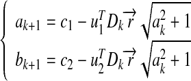
We denote the first and the second rows of A⁺ by u^T₁ and u^T₂, and denote the first and second elements of by c₁ and c₂. By substituting them into (7), we obtain the explicit computing process:

9

At the end of the kth iteration, if D_k does not change, i.e. the position relationships between the target line and all the circle centers are determined, then

10

A necessary condition for the convergence of the iterative process (9) is .

Next we investigate the convergence rate. We denote the accurate solution of the current problem by a_*, and suppose that D_k will no longer change after the kth iteration. Then we have

11

The convergence is therefore of order 1. Let , and the convergent rate is related to . Similarly, we can prove the stability of the solution under convergent conditions. Specifically,

12

Finally, because iterative process (9) involves computing the QR factorization of matrix A_2 × n, its time complexity is .

In view of the above, we know that the essential mathematical issue for orientation detection is to find a feasible solution for the constraint satisfaction problem. However, we know that a neural system is not a digital computer, and solving equations through a computer is not really practical in the neural system. The neural system must apply an equivalent method to solve the problem. A computational circuit is thus the solely natural choice.

Experiments

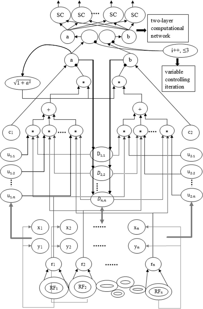
In the previous section, we obtained iterative method (9) which solves for a and b. We have statistically investigated the minimum iteration time required to achieve a specific error bound and the statistical data are given in Table 1. It can be seen that this method reaches an acceptable accuracy (0.001) with a small number of iterations (less than 3). Recurrent networks are quite appropriate for the implementation of iterative computation. By combining the connections between the GCs and the SCs, we derive a neural computational circuit. As shown in Fig. 8, the computing task for each computational unit is mathematically a smooth curve for the sake of easy implementation.

Table 1.

The computing time for the desired error bounds

Error bound	1e − 12	1e − 10	1e − 8	1e − 3
Average iteration time	7.46	6.29	5.42	2.67

Fig. 8.

A recurrent network for orientation calculation. Lines with arrow ends represent excitatory connections (+) while lines with round ends represents inhibitory connections (−).u_i,j denotes the jth element of u^T_i

Here, some representative experiments are conducted to verify the correctness and precision of our approach. These experiments concern the rebuilding of complex polygons and natural images.

Boundary rebuilding of polygons

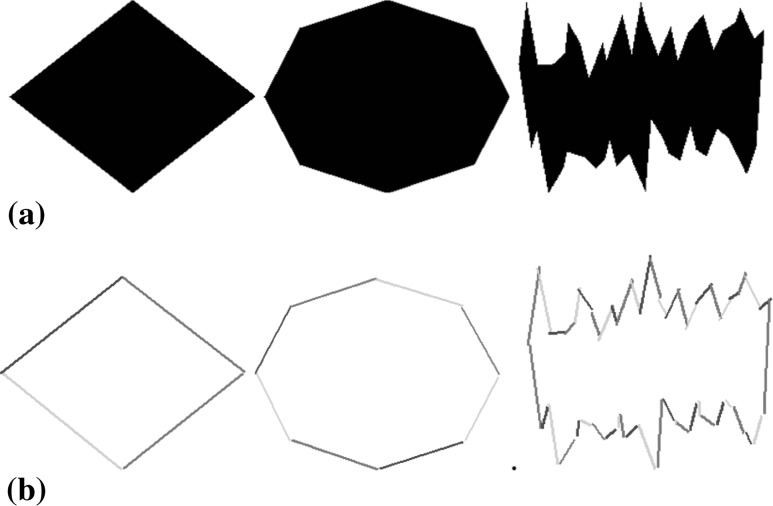
In the x − y plane, n points are chosen, indicated as . These points are connected to format a closed polygon and this polygon is regarded as a stimulus. Then, the RFs of the GCs (in Fig. 9) are distributed on the stimulus. According to the physiological finding on retinas, the sizes of the RFs increase gradually with the increment of the centrifugal degree. From each RF, a circular speculation is generated and its center coordinates and its radius are saved. After all of the RFs have made their predictions, the view is divided into many small regions, and the trained neural network discussed in section “Single ganglion-cell modeling" is used to process every region iteratively. For each region, the RFs’ circular speculations serve as the inputs to the network, and the outputs of the network are the predicted boundary parameters. The experimental results shown in Fig. 10 reveals that the linear edges can be found properly by the proposed model.

Fig. 9.

A typical distribution of neuronal RFs

Fig. 10.

The results of polygon rebuilding. Colors are used to separate detected lines. a Original images of complex polygon. b Boundaries genrated by collective estimation. (Color figure online)

Explanations of visual illusions

In this group of experiments, our algorithms are examined with several optical illusive images.

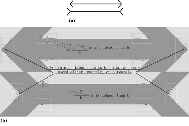
The Müller-Lyer illusion is used first. This experiment tests how our model can be used to explain the occurrence of the Müller-Lyer illusion. As shown in Fig. 11a, two line segments are of identical length but the upper line seems to be shorter than the lower line. The illusion must appear somewhere around the intersections. We generate two images of the enlarged simplified Müller-Lyer illusion, and then run the algorithm over several corner regions. Selected corners are designated with green windows. The detected lines are drawn in purple. Figure 11b illustrates the results with geometrical analyses. The results obtained with the above line occurred in a slightly inward manner, thus shortening the horizontal line. Those below occurred in a slightly outward manner, thus lengthening the horizontal line. The results turn out to be in accordance with the observers’ perceptions.

Fig. 11.

The Müller-Lyer illusion and the explanations. a The Müller-Lyer illusion. b Geometric analyses of the Müller-Lyer illusion. Two detected lines (results) are marked by a ‘a’, and the actual lines (targets) are drawn in red and marked by ‘b’. This diagram shows why the lines are perceived to be longer/shorter around the corners. The relative length of each line between the arrows is meaningless. (Color figure online)

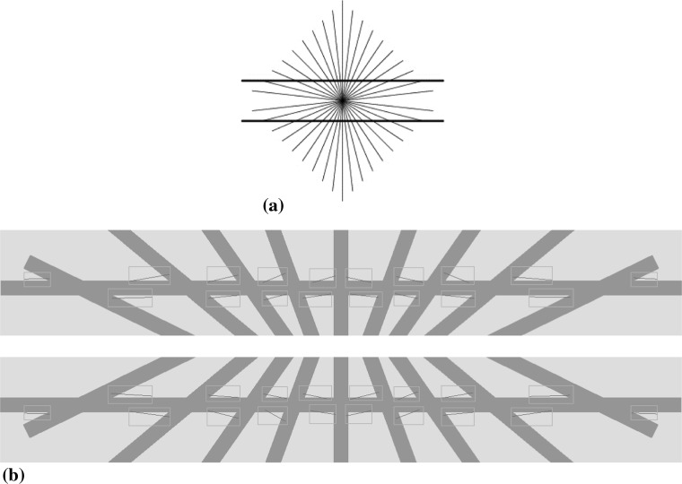
The Hering illusion is used next. As shown in Fig. 12a, the Hering illusive image contains two long parallel lines which are densely intersected by many segments. It seems that the two parallel lines are bending away from each other at the center, as all the acute angles are exaggerated by the eyes. We simplify this image by reducing several segments and enlarge two segmentations containing all of the intersections. Again, we examine our algorithm over the corners, where parts of the long lines are to be detected with short distracting segments.

Fig. 12.

The Hering illusion and the explanations. a The Hering illusion. b Geometric analyses of the Hering illusion. Selected corners are designated with green windows and detected lines are drawn in purple

Natural image experiments and the evaluations

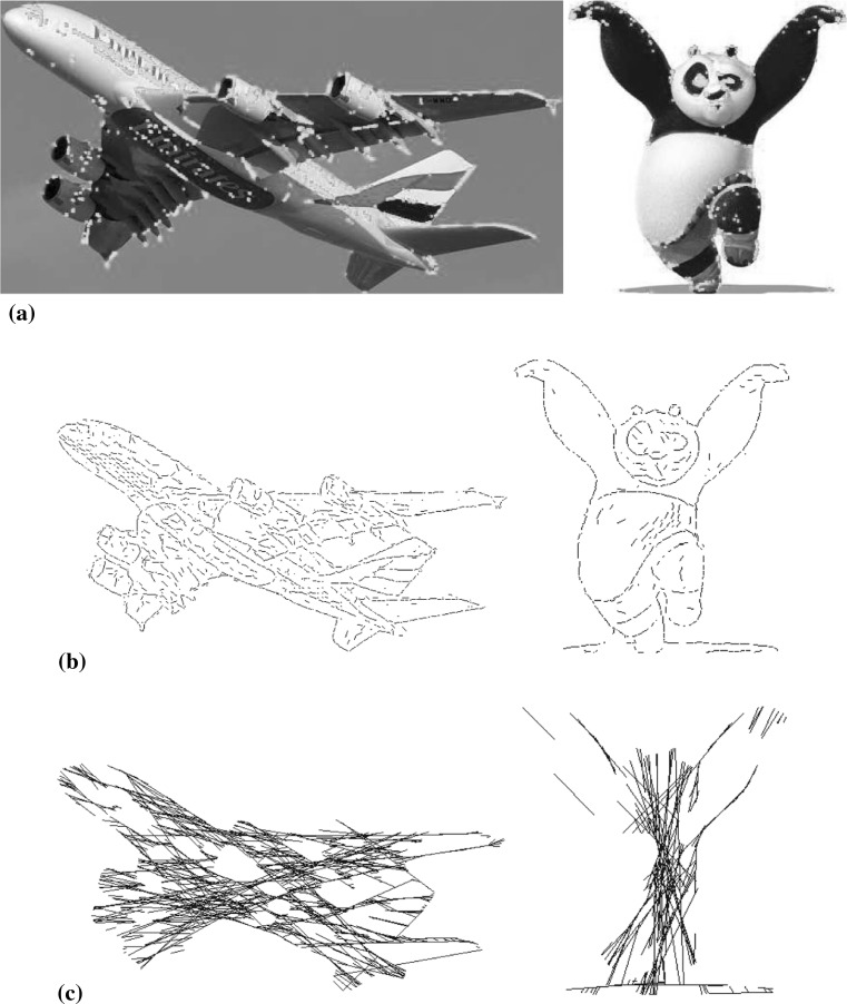
The RFs of an SC’s afferent GCs can be regarded as a window within which an orientation is detected. Sufficient windows can therefore piecewise detect the orientations within a natural image when they cover the entire image. Two examples are illustrated in Fig. 13b. The corresponding results obtained with the Hough transform, a traditional approach for line detection, are illustrated in Fig. 13c. In terms of accuracy, it is quite apparent that the current approach outperforms the Hough transform. Our results contain fewer mistaken lines, which are neither the internal nor the external contours of the objects in the images.

Fig. 13.

The corner maps, the orientation maps and the line maps of two images. a Key points (in light green) obtained with SUSAN corner detection algroithm. Left: A380 airplane. Right: Kung Fu Panda. b Orientation maps obtained with our approach. c Line maps obtained with Hough Transform. (Color figure online)

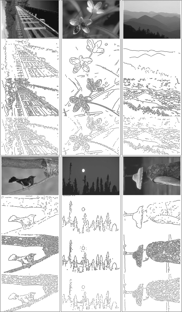
Furthermore, boundary detection is conducted on more challenging natural images. Our algorithm does not aim just to extract the key orientation information which constitutes the semantic framework of tan object, but to remove the insignificant elements which barely play a role in scene understanding. For comparisons, our algorithm, edge detection with Canny operator (Medina-Carnicer et al. 2011) and line detection with Hough transform (Zhang and Webber 1996) are all performed in the same windows.

This paper takes the BSDS500 (Martin et al. 2001) which has been a benchmark for segmentation/recognition as a test set. Fig. 14 illustrates several images and the experiment results. It is obvious that the orientation maps are not just cleaner than the corresponding edge/line maps but preserve more complete essential clues for recognition. It is worth noting that for the texture regions, our algorithm can suppress most undesirable local orientations. The short segments largely existing in the textures are insignificant for understanding the scenes.

Fig. 14.

Boundary detection. In each cell from the top down are: original image from the BSDS500 dataset, its orientation map, Canny-edge map and Hough-line map

Statistical evaluations

Cost-effectiveness

To make a quantitative comparison, we propose an evaluation criterion: the ratio of effectiveness to cost. A corner is the intersection of two edges, and is an important feature in an image. Corners can be found by many corner detection algorithms. As seen in Fig. 13a, a corner usually indicates the existence of two significant line segments which are parts of lines or curves. Let the number of all detected corners be n_c, and the number of them that appear (as black points) in the orientation/line map be n_d, n_d/n_c then measures the computational effectiveness. Nevertheless, because all line detectors will judge more lines when the thresholds are lowered, the effectiveness alone is not enough to evaluate the approach. Let the number of the pixels in the image be n_p and that of the valid points (on lines, black) in the orientation/line map be n_l, n_p/n_l measures the computational cost. A cost-effective detector should have higher .

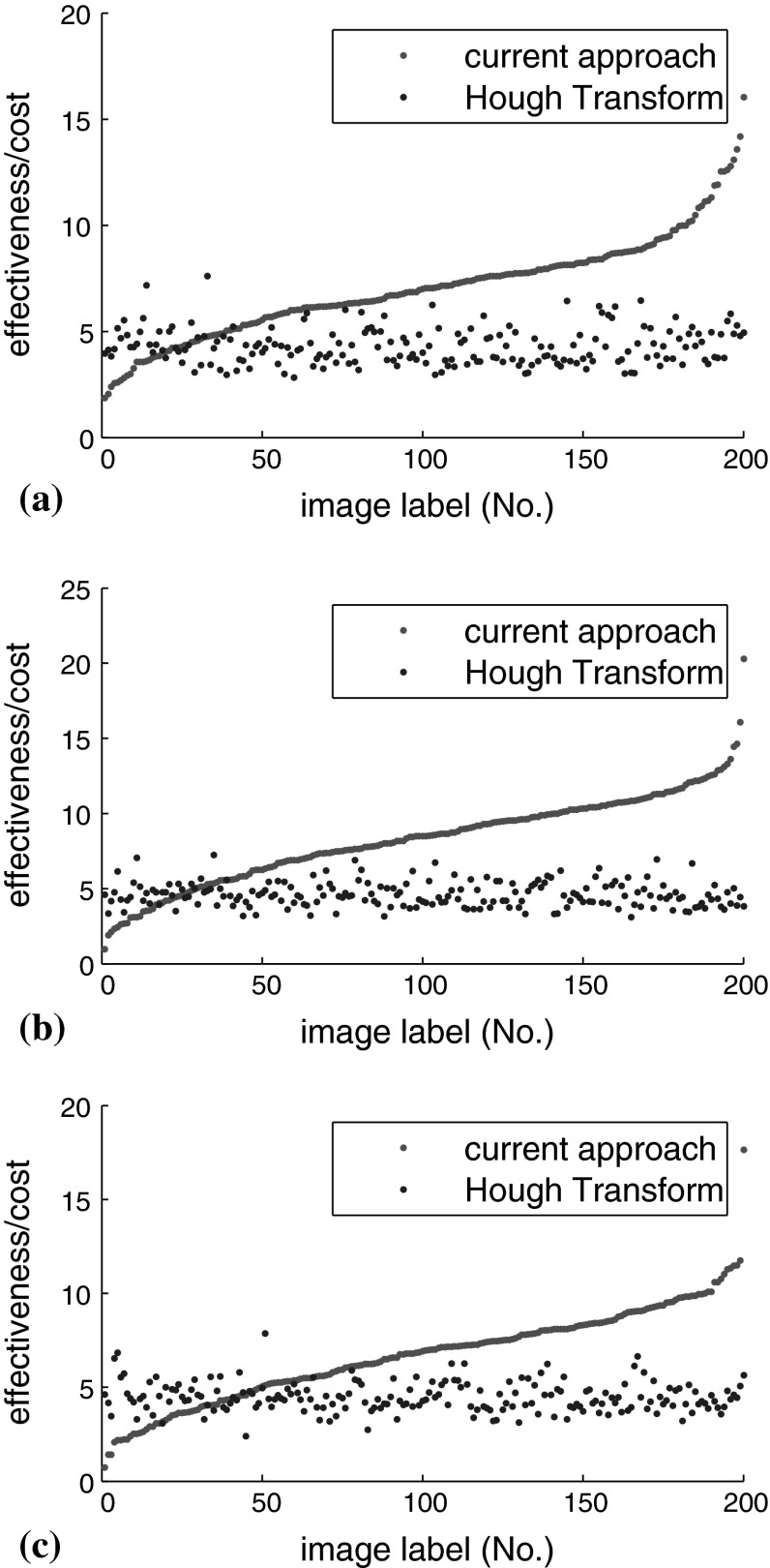
This paper takes 200 test images from the BSDS500 and makes statistics of the effectiveness/cost of the two approaches. Because corner detectors differ in their definitions of corners, and for the sake of objectivity, the comparisons are made using three popular algorithms: SUSAN (Smith and Brady 1997), Harris (Harris and Stephens 1988) and minimum eigenvalue (Shi and Tomasi 1994) algorithms.

As shown in Fig. 15, the three statistical curves further prove that the current approach outperforms the Hough transform in most cases. Our algorithm greatly eliminates false edges and finds a majority of significant contour lines. In contrast, the lines found by Hough transform cannot reflect the real topological structures of the objects. For example, the line map of the “Kung Fu Panda” image contains several through-top-down lines which do not exist in the real image. The results of Hough transform are affected by the parameters in this algorithm and the preprocessing algorithm, i.e. edge detection, and are therefore unstable.

Fig. 15.

The effectiveness-cost curves of the proposed algorithm and Hough transform obtained with different corner maps. The image label numbers are rearranged to make ascending curves of our algorithm. a With SUSAN corner detector. b With Harris corner detector. c With minimum-eigenvalue corner detector

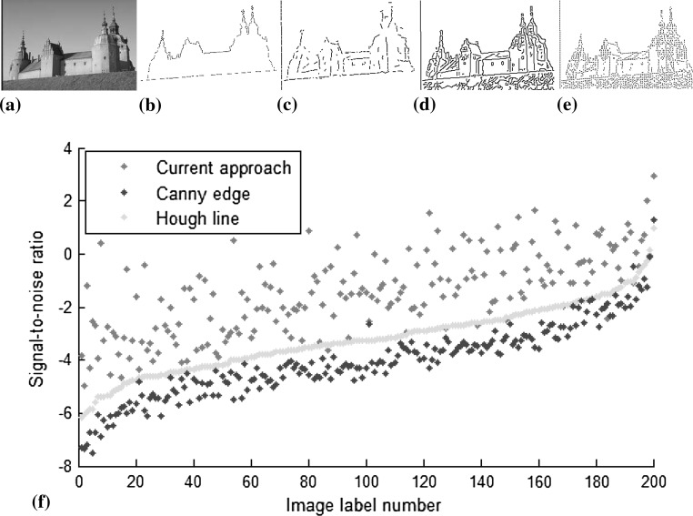
Signal-to-noise ratio

Although the BSDS500 dataset Arbeláez et al. (2011) is mainly for image segmentation, the groundTruth contains the most significant contours of the objects in the images. Too many details will bring side-effect that disturbs segmentation and recognition. In order to test whether our approach can find the most important boundaries and to measure the redundant degree of the obtained information, we take the groundTruth as the standard references. Thus the differences between the references and the corresponding results obtained with each approach are the noise. The signal-to-noise ratio (SNR) given below is defined as in Russ (2011), and the statistical curves are shown in Fig. 16. It is obvious that the current work is more efficient in attracting the semantics of images than the other two approaches.

13

where σ denotes the standard deviation.

Fig. 16.

The results obtained with one image (201080.jpg) in the BSDS500-test and the statistical curves obtained with all images. a Origin. b Ground. c Current. d Canny. e Hough. f The SNR statistcal curves obtained with BSDS500. The image label numbers are adjusted to make an ascending curve of Hough transform

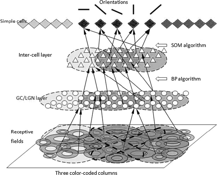
Pinwheel simulation

Figure 17 shows a four-layer neural computational model for orientation calculation. The first layer has photoreceptors where RFs of the GCs are located. The second layer has GCs/LGN cells that are clustered in different groups. The third layer has inter-cells that are also clustered. The fourth layer has simple cells that selectively respond to orientations. The colors purple, green and red in Fig. 17 mark three different orientation columns, respectively, which are partially overlapped. The SOM algorithm is applied between the second and the third layers to train and to localize the approximate scope of an inter cell’s RF. The back propagation (BP) algorithm is applied between the third and the fourth layer to train a simple cell’s response to the two parameters, the slope of a straight line and its ordinate at the origin.

Fig. 17.

A neural network model of collective decision-making

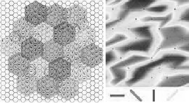
Here we prove that based on the ensemble fitting mechanism this model can also generate an orientation column in the visual cortex. Figure 18 presents the simulation result. Each small hexagon is a simple cell and 19 hexagons constitute a column of orientations. All columns are drawn in different colors. In each column we find all orientations between 0° and 180°. Specifically, at the juncture of several columns, pinwheels (marked by red circles) come into being. On the right is the orientation map drawn with pseudo colors.

Fig. 18.

Pinwheels can be generated by our neural computational model

Discussion

The criterion for biological evolution is “no better than barely enough “or”knowing when to stop”. The neural system is also a product of evolution, and thus it should obey this discipline: its structure should meet its functional demand without over-evolution. We believe that it is luxurious for RFs to be distributed coaxially and lined up equally in all directions, because it places a very high demand on the neural connections. This will then surely put pressure on the evolution of the neural system. In contrast to this highly ordered arrangement, a random structure is much less expensive. Therefore, if a simple structure can work well, then it is not necessary to evolve a complex one.

The findings in neurobiology obtained with stain or fluorescence labeling techniques could only prove the projection directions of neural connections, but they could not explain the meanings of the signals transmitted using these connections. Because of the noise and the scope of the recording, electrophysiological recording of a single electrode could not explain the meaning of the data or the control carried by the signals. Because of the complexity of signal decomposition and temporal coding, multi-channel electrophysiological recording is also insufficient to explain the computational meaning of coding. This means that there is still not enough evidence to prove whether either the geometrical model or algebraic model is absolutely impossible.

In this paper, Hubel-Wiesel hypothesis is considered to be more rigorous under the initial conditions, but our method of fitting the orientation by collective estimation is gentle. In mathematical terms, this method is a single-object optimization under constraints, and has a low computing complexity. It conforms to the common perspective that perception is a type of subjective operation of reconstruction. It can also be implemented with parallel distributed processing, and the precision is acceptable. Table 2 summarized the main difficulties of Hubel-Wiesel model and the proposed improvements in this paper.

Table 2.

The comparisons between Hubel-Wiesel model and our model

Aspect	Difficulties of Hubel-Wiesel model	Proposed improvements
Anatomical	The RF of a GC/LGN cell is constructed by many photoreceptors through horizontal cells and bipolar cells. On such a small scale, it is hardly possible that the RFs of several GCs/LGN cells are distributed collinearly	The RFs of GCs/LGN cells are not necessarily distributed along a line, and these RFs are not required to have the same size
Mathematical	If the RFs of the afferent LGN cells are distributed along a line, the SC can hardly distinguish two stimuli symmetric with respect to the line because they induce the same responses of these LGN cells	The RFs of GCs/LGN cells are not distributed collinearly. An optimization method is proposed for detecting the orientation of the stimulus, and the optimal solution is unique
Physical	It is quite rare that the boundaries of a bar of stimulus are tangent to all the RF centers. The stimulus pattern described in Hubel-Wiesel model cannot account for most ordinary stimuli	The current model considers contrast edges which are the most common type of stimuli in the visual scenes and nature images

Neural systems generate inner representation for the external world, and this representation are used to accomplish many tasks such as scene understanding, object recognition and visual tracking. The neural systems should balance two competing goals: the quality of the representation and the hardware and time costs. The discoveries of place cells and grid cells in the brain (Doeller et al. 2010) precisely indicate that the neural systems can refer to limitedly rough representations and can predict the environment based on multiple cells’ outputs. The prediction accuracy of a single GC or LGN cell is coarse and localized, but these cells are rich in quantity and are shareable. The mechanism, based on these characteristics and an information-integration method, is consistent in logic, rational in psychology, and feasible in physiology. This indicates its significance in cognition. The network design in this paper is enlightened by the projection relation and the RF characteristics of the GCs, LGN cells and V1 cells. Our future research will focus on the integration of related evidence in anatomy, electrophysiology and animal behaviors into the computational model. Information on detected lines will be integrated mainly by V2, V4 and other higher visual areas to determine the ownerships of the lines, and this integration also requires visual attention (Zhou et al. 2000; Qiu et al. 2007; Ito and Komatsu 2004). We will also deal with these issues.

References

- Alexander D, Van Leeuwen C. Mapping of contextual modulation in the population response of primary visual cortex. Cogn Neurodyn. 2010;4:1–24. doi: 10.1007/s11571-009-9098-9. [DOI] [PMC free article] [PubMed] [Google Scholar]
- Alonso JM, Usrey WM, Reid RC. Rules of connectivity between geniculate cells and simple cells in cat primary visual cortex. J Neurosci. 2001;21(11):4002–4015. doi: 10.1523/JNEUROSCI.21-11-04002.2001. [DOI] [PMC free article] [PubMed] [Google Scholar]
- Arbeláez P, Maire M, Fowlkes C, Malik J. Contour detection and hierarchical image segmentation. IEEE Trans Pattern Anal Mach Intell. 2011;33(5):898–916. doi: 10.1109/TPAMI.2010.161. [DOI] [PubMed] [Google Scholar]
- Bhaumik B, Mathur M. A cooperation and competition based simple cell receptive field model and study of feed-forward linear and nonlinear contributions to orientation selectivity. J Comput Neurosci. 2003;14(2):211–227. doi: 10.1023/A:1021911019241. [DOI] [PubMed] [Google Scholar]
- Cai D, Tao L, Shelley M, McLaughlin DW. An effective kinetic representation of fluctuation-driven neuronal networks with application to simple and complex cells in visual cortex. Proc Natl Acad Sci USA. 2004;101(20):7757–7762. doi: 10.1073/pnas.0401906101. [DOI] [PMC free article] [PubMed] [Google Scholar]
- Craft E, Schütze H, Niebur E, von der Heydt R. A neural model of figurecground organization. J Neurophysiol. 2007;97(6):4310–4326. doi: 10.1152/jn.00203.2007. [DOI] [PubMed] [Google Scholar]
- Delorme A, Thorpe SJ. Face identification using one spike per neuron: resistance to image degradations. Neural Netw. 2001;14(6–7):795–803. doi: 10.1016/S0893-6080(01)00049-1. [DOI] [PubMed] [Google Scholar]
- Doeller CF, Barry C, Burgess N. Evidence for grid cells in a human memory network. Nature. 2010;463(7281):657–687. doi: 10.1038/nature08704. [DOI] [PMC free article] [PubMed] [Google Scholar]
- Einevoll G, Plesser H (2012) Extended difference-of-gaussians model incorporating cortical feedback for relay cells in the lateral geniculate nucleus of cat. Cogn Neurodyn 6(4):307–324 [DOI] [PMC free article] [PubMed]
- Enroth-Cugell C, Robson JG. The contrast sensitivity of retinal ganglion cells of the cat. J Physiol Lond. 1966;187(3):517–552. doi: 10.1113/jphysiol.1966.sp008107. [DOI] [PMC free article] [PubMed] [Google Scholar]
- Ferster D, Miller KD. Neural mechanisms of orientation selectivity in the visual cortex. Annu Rev Neurosci. 2000;23:441–471. doi: 10.1146/annurev.neuro.23.1.441. [DOI] [PubMed] [Google Scholar]
- Fukushima K. Neural network model for completing occluded contours. Neural Netw. 2010;23(4):528–540. doi: 10.1016/j.neunet.2009.10.002. [DOI] [PubMed] [Google Scholar]
- Gardner JL, Anzai A, Ohzawa I, Freeman RD. Linear and nonlinear contributions to orientation tuning of simple cells in the cats striate cortex. Vis Neurosci. 1999;16:1115–1121. doi: 10.1017/S0952523899166112. [DOI] [PubMed] [Google Scholar]
- Gomes HM (2002) Model learning in iconic vision. PhD thesis, University of Edinburgh
- Gong HY, Zhang YY, Liang PJ, Zhang PM. Neural coding properties based on spike timing and pattern correlation of retinal ganglion cells. Cogn Neurodyn. 2010;4:337–346. doi: 10.1007/s11571-010-9121-1. [DOI] [PMC free article] [PubMed] [Google Scholar]
- Grigorescu C, Petkov N, Westenberg MA. Contour and boundary detection improved by surround suppression of texture edges. Image Vis Comput. 2004;22:609–622. doi: 10.1016/j.imavis.2003.12.004. [DOI] [Google Scholar]
- Hansen T, Baratoff G, Neumann H. A simple cell model with dominating opponent inhibition for robust contrast detection. Kognitionswissenschaft. 2000;9(2):93–100. [Google Scholar]
- Harris C, Stephens M (1988) A combined corner and edge detector. In: Proceedings of the 4th alvey vision conference, pp 147–151
- Hennig MH, Funke K. A biophysically realistic simulation of the vertebrate retina. Neurocomputing. 2001;38–40:659–665. doi: 10.1016/S0925-2312(01)00426-X. [DOI] [Google Scholar]
- Ito M, Komatsu H. Representation of angles embedded within contour stimuli in area v2 of macaque monkeys. J Neurosci. 2004;24(13):3313–3324. doi: 10.1523/JNEUROSCI.4364-03.2004. [DOI] [PMC free article] [PubMed] [Google Scholar]
- Itti L, Koch C. Computational modelling of visual attention. Nat Rev Neurosci. 2001;2(3):194–203. doi: 10.1038/35058500. [DOI] [PubMed] [Google Scholar]
- Jing W, Liu WZ, Gong XW, Gong HQ, Liang PJ. Visual pattern recognition based on spatio-temporal patterns of retinal ganglion cells activities. Cogn Neurodyn. 2010;4:179–188. doi: 10.1007/s11571-010-9119-8. [DOI] [PMC free article] [PubMed] [Google Scholar]
- Kang S, Lee SW. Real-time tracking of multiple objects in space-variant vision based on magnocellular visual pathway. Pattern Recogn. 2002;35(10):2031–2040. doi: 10.1016/S0031-3203(01)00200-X. [DOI] [Google Scholar]
- Kara P, Pezaris JS, Yurgenson S, Reid RC (2002) The spatial receptive field of thalamic inputs to single cortical simple cells revealed by the interaction of visual and electrical stimulation. Proc Natl Acad Sci USA 99(25):16,261–16,266 [DOI] [PMC free article] [PubMed]
- Kolesnik M, Barlit A, Zubkov E (2002) Simple cell interaction for iterative contrast detection. In: IEEE international conference on artificial intelligence systems, pp 122–128
- Lauritzen TZ, Miller KD (2003) Different roles for simple-cell and complex-cell inhibition in V1. J Neurosci 23(32):10201–10213 [DOI] [PMC free article] [PubMed]
- Lee AB, Blais B, Shouval HZ, Cooper LN (2000) Statistics of lateral geniculate nucleus (LGN) activity determine the segregation of ON/OFF subfields for simple cells in visual cortex. Proc Natl Acad Sci USA 97(23):12875–12879 [DOI] [PMC free article] [PubMed]
- Liu Bh, Li P, Sun YJ, Li Yt, Zhang LI, Tao HW. Intervening inhibition underlies simple-cell receptive field structure in visual cortex. Nat Neurosci. 2010;13(1):89. doi: 10.1038/nn.2443. [DOI] [PMC free article] [PubMed] [Google Scholar]
- Long L, Li Y (2008) Contour detection based on the property of orientation selective inhibition of non-classical receptive field. In: IEEE conference on cybernetics and intelligent systems, 2008, pp 1002–1006
- Martin D, Fowlkes C, Tal D, Malik J (2001) A database of human segmented natural images and its application to evaluating segmentation algorithms and measuring ecological statistics. In: Proceedings of the international conference on computer vision, vol 2, pp 416–423
- McAdams CJ, Reid RC (2005) Attention modulates the responses of simple cells in monkey primary visual cortex. J Neurosci 25(47):11023–11033 [DOI] [PMC free article] [PubMed]
- McKinstry JL, Guest CC (2001) Long range connections in primary visual cortex: a large scale model applied to edge detection in gray-scale images. In: Proceedings of international joint conference on neural networks, 2001, IJCNN ’01, vol 2, pp 843–847
- Medina-Carnicer R, Munoz-Salinas R, Yeguas-Bolivar E, Diaz-Mas L. A novel method to look for the hysteresis thresholds for the Canny edge detector. Pattern Recogn. 2011;44(6):1201–1211. doi: 10.1016/j.patcog.2010.12.008. [DOI] [Google Scholar]
- Mihalas S, Dong Y, von der Heydt R, Niebur E. Mechanisms of perceptual organization provide auto-zoom and auto-localization for attention to objects. Proc Nat Acad Sci. 2011;108(18):7583–7588. doi: 10.1073/pnas.1014655108. [DOI] [PMC free article] [PubMed] [Google Scholar]
- Miikkulainen R, Bednar JA, Choe Y, Sirosh J (2005) Computations in visual maps. In: Computational maps in the visual cortex. Springer, New York, pp 307–324
- Morillasa C, Romero S, Martłnez A, Pelayo F, Reyneri L, Bongard M, Fernndez E. A neuroengineering suite of computational tools for visual prostheses. Neurocomputing. 2007;70(16–18):2817–2827. doi: 10.1016/j.neucom.2006.04.017. [DOI] [Google Scholar]
- Niu WQ, Yuan JQ. Recurrent network simulations of two types of non-concentric retinal ganglion cells. Neurocomputing. 2007;70(13–15):2576–2580. doi: 10.1016/j.neucom.2007.01.008. [DOI] [Google Scholar]
- Norheim E, Wyller J, Nordlie E, Einevoll G (2012) A minimal mechanistic model for temporal signal processing in the lateral geniculate nucleus. Cogn Neurodyn 6(3):259–281 [DOI] [PMC free article] [PubMed]
- Qiu FT, Sugihara T, von der Heydt R. Figure-ground mechanisms provide structure for selective attention. Nat Neurosci. 2007;10(11):1492–1499. doi: 10.1038/nn1989. [DOI] [PMC free article] [PubMed] [Google Scholar]
- Rich TC, Fagan KA, Tse TE, Schaack J, Cooper DMF, Karpen JW (2001) A uniform extracellular stimulus triggers distinct cAMP signals in different compartments of a simple cell. Proc Natl Acad Sci USA 98(23):13049–13054 [DOI] [PMC free article] [PubMed]
- Rodieck RW. Quantitative analysis of cat retinal ganglion cell response to visual stimuli. Vision Res. 1965;5(12):583–601. doi: 10.1016/0042-6989(65)90033-7. [DOI] [PubMed] [Google Scholar]
- Russ JC (2011) The image processing handbook, 6th edn. CRC Press, New York, chap 6, p 376
- Sajda P, Baek K. Integration of form and motion within a generative model of visual cortex. Neural Netw. 2004;17(5C6):809–821. doi: 10.1016/j.neunet.2004.03.013. [DOI] [PubMed] [Google Scholar]
- Sakai K, Nishimura H. Surrounding suppression and facilitation in the determination of border ownership. J Cogn Neurosci. 2006;18(4):562–579. doi: 10.1162/jocn.2006.18.4.562. [DOI] [PubMed] [Google Scholar]
- Serre T, Wolf L, Bileschi S, Riesenhuber M, Poggio T. Robust object recognition with cortex-like mechanisms. IEEE Trans Pattern Anal Mach Intell. 2007;29(3):411–426. doi: 10.1109/TPAMI.2007.56. [DOI] [PubMed] [Google Scholar]
- Shi J, Tomasi C (1994) Good features to track. In: Proceedings of IEEE computer society conference on computer vision and pattern recognition, pp 593–600
- Smith SM, Brady JM. Susan-new approach to low level image processing. Int J Comput Vision. 1997;23:45–78. doi: 10.1023/A:1007963824710. [DOI] [Google Scholar]
- Smyth D, Willmore B, Baker GE, Thompson ID, Tolhurst DJ. The receptive-field organization of simple cells in primary visual cortex of ferrets under natural scene stimulation. J Neurosci. 2003;23(11):4746–4759. doi: 10.1523/JNEUROSCI.23-11-04746.2003. [DOI] [PMC free article] [PubMed] [Google Scholar]
- Sompolinsky H, Shapley R. New perspectives on the mechanisms for orientation selectivity. Curr Opin Neurobiol. 1997;7(4):514–522. doi: 10.1016/S0959-4388(97)80031-1. [DOI] [PubMed] [Google Scholar]
- Stephen D, Jack G. Predicting neuronal responses during natural vision. Netw Comput Neural Syst. 2005;16(2–3):239–260. doi: 10.1080/09548980500464030. [DOI] [PubMed] [Google Scholar]
- Tang H, Li H, Yi Z. Online learning and stimulus-driven responses of neurons in visual cortex. Cogn Neurodyn. 2011;5:77–85. doi: 10.1007/s11571-010-9143-8. [DOI] [PMC free article] [PubMed] [Google Scholar]
- Tao L, Shelley M, McLaughlin D, Shapley R. An egalitarian network model for the emergence of simple and complex cells in visual cortex. Proc Natl Acad Sci USA. 2004;101(1):366–371. doi: 10.1073/pnas.2036460100. [DOI] [PMC free article] [PubMed] [Google Scholar]
- Troyer TW, Krukowski AE, Miller KD. LGN input to simple cells and contrast-invariant orientation tuning: an analysis. J Neurophysiol. 2002;87(6):2741–2752. doi: 10.1152/jn.2002.87.6.2741. [DOI] [PubMed] [Google Scholar]
- Wagatsuma N, Shimizu R, Sakai K. Independence of space-based and feature-based attention in the determination of figure direction. BMC Neurosci. 2008;9(Suppl 1):116. doi: 10.1186/1471-2202-9-S1-P116. [DOI] [Google Scholar]
- Wallis G. Linear models of simple cells: correspondence to real cell responses and space spanning properties. Spat Vis. 2001;14(3–4):237–260. doi: 10.1163/156856801753253573. [DOI] [PubMed] [Google Scholar]
- Watson AB, Ahumada AJ Jr (1989) A hexagonal orthogonal-oriented pyramid as a model of image representation in visual cortex. IEEE Trans Biomed Eng 36(1):97–106 [DOI] [PubMed]
- Wielaard DJ, Shelley M, McLaughlin D, Shapley R. How simple cells are made in a nonlinear network model of the visual cortex. J Neurosci. 2001;21(14):5203–5211. doi: 10.1523/JNEUROSCI.21-14-05203.2001. [DOI] [PMC free article] [PubMed] [Google Scholar]
- Willmore B, Watters PA, Tolhurst DJ. A comparison of natural-image-based models of simple-cell coding. Perception. 2000;29(9):1017–1040. doi: 10.1068/p2963. [DOI] [PubMed] [Google Scholar]
- Yang S, Wu Q, Li R. A case for spiking neural network simulation based on configurable multiple-fpga systems. Cogn Neurodyn. 2011;5:301–309. doi: 10.1007/s11571-011-9170-0. [DOI] [PMC free article] [PubMed] [Google Scholar]
- Zhang Y, Webber R. A windowing approach to detecting line segments using hough transform. Pattern Recogn. 1996;29(2):255–265. doi: 10.1016/0031-3203(95)00083-6. [DOI] [Google Scholar]
- Zhou H, Friedman HS, von der Heydt R. Coding of border ownership in monkey visual cortex. J Neurosci. 2000;20(17):6594–6611. doi: 10.1523/JNEUROSCI.20-17-06594.2000. [DOI] [PMC free article] [PubMed] [Google Scholar]