Abundance and Distribution of Transposable Elements in Two Drosophila QTL Mapping Resources

Abstract

Here we present computational machinery to efficiently and accurately identify transposable element (TE) insertions in 146 next-generation sequenced inbred strains of Drosophila melanogaster. The panel of lines we use in our study is composed of strains from a pair of genetic mapping resources: the Drosophila Genetic Reference Panel (DGRP) and the Drosophila Synthetic Population Resource (DSPR). We identified 23,087 TE insertions in these lines, of which 83.3% are found in only one line. There are marked differences in the distribution of elements over the genome, with TEs found at higher densities on the X chromosome, and in regions of low recombination. We also identified many more TEs per base pair of intronic sequence and fewer TEs per base pair of exonic sequence than expected if TEs are located at random locations in the euchromatic genome. There was substantial variation in TE load across genes. For example, the paralogs derailed and derailed-2 show a significant difference in the number of TE insertions, potentially reflecting differences in the selection acting on these loci. When considering TE families, we find a very weak effect of gene family size on TE insertions per gene, indicating that as gene family size increases the number of TE insertions in a given gene within that family also increases. TEs are known to be associated with certain phenotypes, and our data will allow investigators using the DGRP and DSPR to assess the functional role of TE insertions in complex trait variation more generally. Notably, because most TEs are very rare and often private to a single line, causative TEs resulting in phenotypic differences among individuals may typically fail to replicate across mapping panels since individual elements are unlikely to segregate in both panels. Our data suggest that “burden tests” that test for the effect of TEs as a class may be more fruitful.

Introduction

Transposable elements are common, naturally occurring sources of genetic variation known to play diverse roles in genome evolution (Bennetzen 2000; reviewed in Kazazian 2004), influencing chromosomal rearrangements (Lonnig and Saedler 2002; Biemont and Vieira 2006), genome size (Kidwell 2002) and gene duplication (Schmidt et al. 2010). They also contribute both to functional variation between individuals (Daborn et al. 2001; Aminetzach et al. 2005) and to tissue-specific gene expression (Sackton et al. 2009). TEs can also contribute to variation in quantitative traits such as bristle number variation (Mackay 1984; Shrimpton et al. 1990; Mackay et al. 1992) and fitness (Mackay 1989). However, this variation is not limited to the production of null alleles, but instead TEs can produce a wide variety of changes in gene expression. TEs can act as enhancers (Chung et al. 2007), repressors (Zachar and Bingham 1982), or regulators of more complex expression patterns acting either in cis or in trans (Smith and Corces 1991). Additionally, different TE insertions into the same gene do not necessarily produce the same effect (Zachar and Bingham 1982; Birchler et al. 1989; Birchler and Hiebert 1989).

In Drosophila, a large portion of phenotypic variation is likely due to rare alleles maintained through mutation-selection balance (Mackay 2010). TEs are potentially good candidates to be rare, causative mutations contributing to a wide variety of phenotypic variation. The population frequency of most TE insertions in Drosophila is low (Charlesworth and Langley 1989), resulting in rare variants that could potentially have phenotypic consequences. TE insertions are often deleterious and host genomes have evolved a variety of methods to regulate TE replication in their genomes (reviewed in Slotkin and Martienssen 2007). Still, many transposable elements are known to be active in Drosophila melanogaster (Deloger et al. 2009), with insertion rates ranging between 10⁻³ and 10⁻⁵ elements per generation (Nuzhdin and Mackay 1994), suggesting high rates of ongoing activity in many different TE families continuing to produce rare variants.

Individually rare transposable element insertions as a class of mutations have also been associated with quantitative traits in Drosophila (Mackay and Langley 1990; Long et al. 2000). TEs as a class have been found to be causative mutations in association studies examining both the Enhancer-of-split gene complex and the achaete-scute complex in Drosophila (Mackay and Langley 1990; Long et al. 2000; Macdonald et al. 2005; Gruber et al. 2007). Future studies may reveal many more examples of TEs as a class as causative mutations.

Recently two reference panels for the mapping of quantitative trait loci (QTL) have been unveiled: the Drosophila Genetic Reference Panel (DGRP) (Mackay et al. 2012) and the Drosophila Synthetic Population Resource (DSPR) (King et al. 2012a, 2012b). The DGRP is a set of 168 inbred isofemale lines derived from individuals collected in Raleigh, NC, in 2003. The DSPR is a collection of ∼1700 Recombinant Inbred Lines derived from 15 highly inbred founder lines. The founders were collected from many different geographic locations and were all been in laboratory conditions for 40+ years (Macdonald and Long 2007). These resources are intended for use as platforms to map QTL in D. melanogaster and have been characterized with respect to single-nucleotide polymorphism (SNP) genotypes (King et al. 2012a; Mackay et al. 2012). In addition, an initial pass at calling transposable element (TE) insertions in the DGRP was presented in Mackay et al. (2012) and in Linheiro and Bergman (2012). This study revealed hundreds of rare TE insertions per line and in cases where TE insertions are found in the same gene in multiple lines, the insertions are usually at different positions within the gene (Mackay et al. 2012). These findings suggest that marker-based associations where the causative mutation is a TE insertion may fail to replicate, and that tests for the effects of TE insertions as a class of mutations, such as in Mackay and Langley (1990), Long et al. (2000), and Macdonald et al. (2005), may be more fruitful.

Replicability of genotype–phenotype associations is a critical step for establishing causative variation and genome-wide association studies in humans use replication in multiple data sets as a standard of quality (NCI-NHGRI Working Group on Replication in Association Studies 2007). Future studies using the DGRP and DSPR must also consider differences in the pattern of TE insertions between panels when designing experiments utilizing these resources because a causative TE segregating in one panel but not in the other would affect the replicability of a study. It is therefore important to know the TE genotype of the individual fly lines used in QTL studies in Drosophila and an accurate characterization of the TE content of both panels is desirable for future QTL mapping studies in Drosophila. Currently, in D. melanogaster, there are only a few replicated associations. One set involves TE insertions at the achaete-scute complex and their effect on bristle number (Mackay and Langley 1990; Long et al. 2000). There is one example of a replicated association involving a SNP and the gene Egfr in Drosophila (Palsson and Gibson 2004; Dworkin et al. 2005), although the nature of the replication is complex because the specific phenotype associated with the replicated SNP differs between studies.

Here we describe the TE content of two QTL mapping resources, identifying patterns of TE abundance and distribution. We find that TEs are generally rare, existing in only one line, and that there is an excess of rare TEs compared with the standard neutral model and SNPs. We find substantial variation between genes in term of TE load as well as a weak effect of gene family size on average TE load on genes. TEs are also at higher densities in regions of low recombination as well as on the X chromosome.

New Approaches

Here we present a whole-genome TE calling method which is an improvement to the method used to call TEs in Mackay et al. (2012) and apply it to two QTL mapping resources (supplementary fig. S1, Supplementary Material online). Briefly, TEs are identified by read-pairs generated via next-generation, paired-end sequencing. Informative read-pairs are characterized by a pattern of one read in the pair aligning uniquely to the genome and the other read in the pair aligning to multiple genomic regions. Individual insertion events are identified by two sets of read pairs, one set anchored by uniquely aligning reads upstream of the insertion and one set anchored by uniquely aligning reads downstream of the insertion. Following identification of informative read pairs, we use Phrap (Ewing and Green 1998) to reconstruct the local area in genomic regions suggestive of the presence of a TE. Reconstructed sequences are then aligned back to the reference genome using BlastN (Altschul et al. 1990) to validate the presence of a TE breakpoint and to classify the type of TE identified.

There are four major improvements to this method over the previous method used in Mackay et al. (2012). First, we have switched to using the aligner BWA (Li and Durbin 2009) which is more accurate at distinguishing unique from non-unique alignments to a reference genome than the Mosaik 1.0 (http://code.google.com/p/mosaik-aligner/downloads/detail?name=Mosaik%201.0%20Documentation.pdf, last accessed June 30, 2012) aligner used in Mackay et al. (2012) for TE detection. Second, we have incorporated bedtools (Quinian and Hall 2010) into our pipeline which has improved the speed at which we can detect events. Third, we have also incorporated definitive absence calls to the pipeline, where we attempt to positively call the presence or absence of a TE at a given position in a given genotype (c.f., Mackay et al. 2012). Finally, we have performed both computational and polymerase chain reaction (PCR)-based validation of our method, demonstrating the method’s precision and sensitivity.

Results

Identity by Descent in the DGRP Resource

Because association studies rely on the assumption that individuals are unrelated (Voight and Pritchard 2005), we used the SNP calls from Mackay et al. (2012) to scan for regions of extensive identity by descent (IBD) in the DGRP sample; >95% similarity in 1 Mb windows with 100 kb steps. We began with a total of 148 DGRP lines for which we have sequence data. We identified many large regions of IBD between pairs of lines (fig. 1A) and removed from the analysis a total of 13 DGRP lines which were identified as ≥95% IBD with another line over ≥50% of their genomes. When two lines showed such genome-wide IBD, the line with the highest average coverage was retained for further analyses. Similarly, regions in remaining DGRP lines which were ≥95% IBD to another line were masked in the line with the lowest average genome coverage. In addition to the regions removed due to IBD, we removed four lines from the DGRP set which had an average genome coverage of <10× (supplementary table S1, Supplementary Material online). This filtering resulted in a sample size of 131 DGRP lines, some of which were partially masked, to be used in all further analyses. This removal of some lines and masking of regions in other lines resulted in variation in sample sizes across the genome. For 98% of sites in the genome, the sample size was ≥68. For the remainder of sites, coverage was low in a substantial number of lines, indicative of genomic regions where alignment of short reads is difficult.

Fig. 1.

(A) Identity by descent in 148 DGRP lines. (B) IBD in the top 15 DGRP lines by average sequence coverage. (C) IBD in the 15 DSPR lines. Masked regions indicate regions of IDB ≥95%. When two lines were considered IBD in a region, the line with lower mean coverage was masked.

Coalescent simulations of an equilibrium Wright–Fisher model showed that the probability of more than four pairs of lines with a single 1 Mb region of IBD matching our IBD criteria is <10⁻³. Therefore, our observation of hundreds of 1 Mb regions of IBD between pairs of lines (fig. 1A) indicated that there was substantially more IBD in the DGRP than expected in a panel of randomly chosen individuals sampled from an idealized population. However, the extent of IBD was similar between the 15 DSPR founder lines and the 15 DGRP lines with the highest average sequence coverage (fig. 1B and C) and was equal to a few dozen megabytes of IBD, including a large proportion of centromeric regions. It is therefore unclear whether the extensive IBD seen in 148 lines of the DGRP (fig. 1A) is a general property of large samples of cosmopolitan D. melanogaster or a specific property of the DGRP line collection.

Data Filtering

Following the IBD analysis, we identified transposable element insertions in a total of 146 lines, 131 DGRP, and 15 DSPR founder lines. TEs identified at a specific genomic location were either present in the D. melanogaster reference sequence (version 5.13, downloaded from www.flybase.org, last accessed January 30, 2009), hereafter referred to as reference TEs, or not present in the reference sequence, hereafter referred to as novel TEs. Centromeric and telomeric regions, defined in the Materials and Methods section, were excluded from the analysis as identification of TEs in these regions can be problematic since their very high TE densities result in few informative read-pairs. In addition, we wished to focus on the euchromatic regions of the genome since most genes are located in these regions. We also removed from the data sets reference TEs which were <75% of a full length copy of the element as these elements are unlikely to be active copies. These filtering steps reduced the number of reference TEs considered in later analysis to 607 from a starting total of 6,003.

Validation of Transposable Element Presence/Absence Calls

Simulation

Detecting a set of inserted elements in silico showed that at an average genome coverage of 50×, we were able to detect 91.3% of elements that were at least 75% of the length of the canonical element. These are the set of events directly comparable to the set of reference TEs we kept for our analysis, since these are the set of TEs that are likely to be active copies in the genome. A drop in average genome coverage did not affect our rate of identification in simulated data sets. We detected 95.6% of elements at 25× coverage and 91.3% of elements at 15× coverage.

When we looked at the detection of all elements, we found that we were able to identify the insertion locations for 70% of all elements at 50× coverage, 72.4% of elements at 25× coverage, and 64% of elements at 15× coverage.

PCR Validation

We compared our pipeline’s TE calls with PCR data from 1,687 PCR calls of TE insertions in 9 of the DGRP lines (Blumenstiel JP, Chen X, He M, Bergman CM, unpublished data, http://arxiv.org/abs/1209.3456, last accessed June 26, 2013). The comparison of our pipeline to PCR-validated insertions showed a 92.4% overall agreement between the two methods (supplementary table S2, Supplementary Material online) when comparing presence and absence calls. We did not include the few examples of heterozygous insertions in this analysis. Our pipeline was unable to make a presence or absence call for the set of PCR-validated insertions 6% of the time and disagreed with the PCR data 1.6% of the time. Failure to validate via PCR was equally likely for presence or absence calls, suggesting that detection of TEs was unbiased with respect to presence versus absence. We estimate a pipeline sensitivity of 98.2% and a specificity of 94% based on this subset of the data. Our estimation of the validation rate is conservative, requiring us to reconstruct a contig that either contains the TE breakpoint or spans over the insertion site in order to call an event as either present or absent, respectively. For some cases where our pipeline makes no call, we did see read pairs that are suggestive of the state of the presence or absence of the TE, but are not sufficient in number and/or uniqueness for reconstruction the event de novo.

Computational Validation

The initial phase of our pipeline detected transposable element insertions in individual lines. Following this initial detection phase, our pipeline surveys every line at each genomic location where a TE insertion was identified in any other line, including lines in different data sets. In this manner we attempted to computationally verify the presence or absence of TE insertions at a total of 2,596,370 genomic locations. Our pipeline made presence or absence calls between 97.17% and 99.98% of the time (supplementary table S3, Supplementary Material online). Positive absence calls made by our pipeline can also be considered a type of validation since to make an absence call our pipeline must detect reads that span the junction where the insertion would be located (supplementary table S3, Supplementary Material online).

The presence of regions of IBD amongst DGRP lines (fig. 1) provided an opportunity to cross-validate TE calls in regions masked as IBD between different line pairs, because we expected TE genotypes to be identical within regions identified as IBD. We find a mean of 98% agreement for TE calls (both presence and absence) between pairs of regions identified as IBD, with a standard deviation of 0.015.

Distribution and Abundance of Transposable Elements

A total of 7,104 transposable element insertions were found in the DSPR and 17,639 in the DGRP. A comparison of the TE insertion content of the DGRP and DSPR reveals that each panel contained a large number of TE insertions specific to that panel; only 1,656 insertions were shared between the DSPR and DGRP data sets out of a total of 23,087 insertions detected (i.e., 7.2% shared insertions). All transposable element insertion locations are listed in supplementary tables S4 and S5, Supplementary Material online. A subset of the DGRP data, lines with an average sequence coverage ≥25×, mean sequence coverage 33.5×, standard deviation 5.1, hereafter DGRP25 (table 1), contained 5,855 insertions. The DGRP25 set of lines was used in some analyses to be more directly comparable to the DSPR lines which all had a mean genome coverage of ≥60× (fig. 2).

Table 1.

Summary of TE Insertions.

	DGRP	DGRP25	DSPR
Total	17,639	5,855	7,104
Not present in reference	17,346	5,615	6,812
Present in reference	293	240	292
X, recombination ≤ 2 cM/Mb	418	149	203
X, recombination > 2 cM/Mb	2,741	948	1,107
Autosomes, recombination ≤ 2 cM/Mb	6,205	2,131	2,694
Autosomes, recombination > 2 cM/Mb	8,177	2,544	3,019
4, all	98	83	81
Exon	1,158	378	633
Intron	8,595	2,870	3,310
3′ UTR	477	159	234
5′ UTR	190	63	81
Intergenic	7,219	2,680	3,269
DNA elements	1,388	514	748
RNA elements	10,133	3,004	4,085
Indeterminate	6,118	2,336	2,271

Fig. 2.

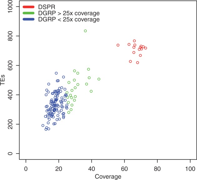
Total number of TEs identified versus coverage for the DGRP, DGRP25, and DSPR lines.

In both resources, TE insertions were generally at low frequency. Overall, we found a larger total number of insertions per line in DSPR than in DGRP (fig. 2). This was presumably due to the much higher sequencing coverage of the former leading to a higher power to make calls of complex insertions. Mean sequence coverage for the DGRP lines was 19.5× with a standard deviation of 6.4; mean sequence coverage for the DSPR was 67.1× with a standard deviation of 4.2. However, the increased amount of time the DSPR lines have remained in laboratory conditions may also have contributed to the elevated number of TEs seen in these lines (Nuzhdin et al. 1997).

TEs may be located at random throughout the genome or they may be found preferentially in certain genomic regions, such as in intergenic sequence. We used the binomial distribution as a null model for the distribution of TEs in the genome, assuming TEs insert and remain at random with respect to these genomic features (table 2). We found that in general the distribution of TEs observed differed from what we would expect if TEs were distributed at random throughout the genome. We found significantly fewer TEs in exons, 5′ UTRs, and 3′ UTRs than expected and significantly more TEs than expected in intergenic and intronic regions (table 2), which was consistent with previous observations as TEs in genes are much more likely to be deleterious (Kaminker et al. 2002; Lipatov et al. 2005). This pattern held true for the DGRP, the DGRP25, and the DSPR suggesting that selection may be acting universally to remove TEs that disrupt exonic sequences.

Table 2.

Differences between Observed and Expected TE Counts.

	DGRP		DGRP25		DSPR
	Observed vs. Expected	P Value	Observed vs. Expected	P Value	Observed vs. Expected	P Value
X, recombination ≤ 2 cM/Mb	Decrease	3.29E−11	Decrease	1.87E−03	Decrease	5.22E−02
X, recombination > 2 cM/Mb	Decrease	1.74E−01	Increase	7.01E−02	Increase	4.16E−01
Autosomes, recombination ≤ 2 cM/Mb	Decrease	3.70E−01	Increase	1.00E+00	Increase	6.87E−04
Autosomes, recombination > 2 cM/Mb	Increase	3.92E−02	Decrease	1.00E+00	Decrease	1.00E+00
Exon	Decrease	0.00E+00	Decrease	2.47E−323	Decrease	1.03E−283
Intron	Increase	3.54E−103	Increase	0.00E+00	Increase	0.00E+00
3′ UTR	Decrease	6.99E−16	Decrease	3.13E−06	Decrease	1.26E−02
5′ UTR	Decrease	1.43E−51	Decrease	2.82E−18	Decrease	4.98E−20
Intergenic	Increase	1.12E−32	Increase	0	Increase	0.00E+00

TE Identification

Information about the class of TE that has been inserted is useful for two reasons. First, this information will allow for rapid assays for the presence of this TE in other strains. Second, insertions of different families of TEs can produce different phenotypic consequences (Smith and Corces 1991). We were able to identify the TE class of the majority of insertions (table 1). RNA elements were much more common than DNA elements, and within RNA elements over half were long terminal repeat (LTR) retrotransposon elements. We were unable to identify element class for 34.7% of the DGRP insertions and 32.0% of the DSPR insertions. In cases where we were unable to identify the TE family for an insertion, this was due to either conflict between the most likely TE as identified by the two reconstructed contigs for each event or because we had limited data on the TE sequence for that event. In cases where we have conflicting information, this was due to 1) the degradation of the TE sequence so that there were many poor matches to multiple families, 2) conserved sequence between families and therefore good matches to multiple families, 3) because we identified a nest of elements where multiple elements insert in very close proximity or within one another, or 4) the amount of TE sequence we were able to reconstruct was less than 80 bp and therefore below our annotation threshold length. Because of the frequently short length of TE sequence that we attempted to identify, we did not attempt to identify the strand of the TE insertion. Although TE orientation is important and influences selection upon the insertion (Cutter et al. 2005), our data were frequently insufficient to resolve strand.

Factors Influencing TE Density

If TE insertions are deleterious and recessive with respect to fitness, then insertions are also predicted to be more common on the autosomes since deleterious insertions on the X will be eliminated via selection against hemizygous males (Charlesworth and Langley 1989). Contrary to this prediction, an analysis of variance (ANOVA) indicated a significant effect of chromosome on mean TE density per line when both resources were included in the same analysis (table 3). This difference was due to an increased mean density of TEs on the X versus the autosomes in regions of high recombination. This pattern was the same both for autosomes taken as a group and for each autosome individually (table 4).

Table 3.

ANOVAs for DSRP and DGRP25 Coverage and Comparison between the Two Data Sets.

	df	Sum Sq.	Mean Sq.	F value	Pr(>F)
DSPR vs. DGRP25
Set	1	541.25	541.25	648.6975	<2e−16
Line	36	284.8	7.91	9.4817	<2e−16
Chromosome	4	118.58	29.65	35.5313	<2e−16
Recombination rate (high vs. low)	1	255.75	255.75	306.5207	<2e−16
Chromosome*recombination rate	4	103.35	25.84	30.9663	<2e−16
Residuals	333	277.84	0.83
DSPR
Line	14	26.599	1.9	1.7894	0.04699
Chromosome	4	39.632	9.908	9.3316	1.23e−06
Recombination rate (high vs. low)	1	141.337	141.337	133.1143	<2e−16
Chromosome*recombination rate	4	39.712	9.928	9.3504	1.19e−06
Residuals	126	133.783	1.062
DGRP25
Line	22	258.202	11.736	17.23	<2e−16
Chromosome	4	80.126	20.031	29.409	<2e−16
Recombination rate (high vs. low)	1	120.011	120.011	176.191	<2e−16
Chromosome*recombination rate	4	66.056	16.514	24.244	2.43e−16
Residuals	198	134.866	0.681

Table 4.

TE Density in the X and Autosomes.

	TE/Mb
	DGRP25	DSPR	Both
X, all	3.82	6.38	4.83
Autosomes, all	3.51	5.93	4.47
X, high recombination	3.71	6.00	4.61
X, low recombination	3.93	6.76	5.05
2L, high recombination	2.27	4.73	3.24
2L, low recombination	3.23	5.89	4.28
2R, high recombination	2.82	4.89	3.64
2R, low recombination	6.17	8.63	7.14
3L, high recombination	2.96	5.23	3.86
3L, low recombination	4.74	7.26	5.73
3R, high recombination	2.81	4.68	3.55
3R, low recombination	3.72	6.70	4.90

TEs are predicted to accumulate in regions of low recombination where they are less likely to produce deleterious rearrangements via ectopic exchange (Charlesworth and Langley 1989). An ANOVA indicates a highly significant effect of recombination rate on mean TE density per line (table 3). TE density was also found to be greater in regions of low recombination than in high recombination throughout the genome, which was consistent with the predictions of Charlesworth and Langley (1989).

Because the factors that influence TE density may differ greatly from family to family, we repeated this analysis in 14 families of TEs that appear in moderate to high abundance in the two resources (table 5). Many of these families were previously examined by Montgomery et al. (1987) and Bartolome et al. (2002).

Table 5.

TE Density for 15 Individual Families of Elements.

		Mean Density (TE/Mb)
Element	Resource	X High	X Low	Auto High	Auto Low
roo	DGRP25	0.39	0.37	0.32	0.33
	DSPR	0.80	0.88	0.65	0.68
297	DGRP25	0.05	0.00	0.02	0.01
	DSPR	0.05	0.00	0.04	0.00
412	DGRP25	0.03	0.01	0.03	0.07
	DSPR	0.06	0.08	0.09	0.12
F	DGRP25	0.02	0.06	0.04	0.06
	DSPR	0.07	0.08	0.12	0.13
17.6	DGRP25	0.01	0.00	0.01	0.02
	DSPR	0.02	0.00	0.02	0.06
Bari1	DGRP25	0.01	0.00	0.04	0.01
	DSPR	0.02	0.02	0.06	0.02
copia	DGRP25	0.01	0.00	0.02	0.03
	DSPR	0.09	0.02	0.14	0.19
H	DGRP25	0.01	0.00	0.01	0.00
	DSPR	0.00	0.00	0.01	0.00
hopper	DGRP25	0.10	0.01	0.00	0.00
	DSPR	0.10	0.04	0.02	0.02
INE-1	DGRP25	0.42	1.88	0.03	0.48
	DSPR	0.45	2.03	0.04	0.55
jockey	DGRP25	0.15	0.12	0.19	0.13
	DSPR	0.35	0.34	0.40	0.33
mdg1	DGRP25	0.03	0.02	0.03	0.10
	DSPR	0.08	0.04	0.12	0.18
pogo	DGRP25	0.06	0.04	0.07	0.05
	DSPR	0.13	0.21	0.15	0.13
springer	DGRP25	0.00	0.01	0.01	0.03
	DSPR	0.02	0.00	0.01	0.05

We found that in 10 families (412, roo, 17.6, F, Bari1, copia, hopper, INE-1, mdg1, springer) there was a highly significant difference in mean TE density between the X and the autosomes (P value ≤0.026 in all cases), although the direction of the difference varied among families. Within these families there were substantial differences. In two of the families, INE-1 and roo, we saw an increased density in the X over the autosomes in regions of high recombination in both the DSPR and DGRP25 resource (table 5). However, for 412, F, mdg1, springer, Bari1, and copia, we saw the opposite pattern. This suggests that there may be substantial variation in TE insertion site preferences among families.

Sample Counts of Transposable Elements

The power to detect an association is dependent both on the penetrance and the frequency of the causal allele (Hirschhorn and Daly 2005). We found that the majority of transposable elements in the DGRP25 and the DSPR are found in only one line (fig. 3). Comparisons between the observed TE data and SNPs from the same population found in introns ≤86 bp (Haddrill et al. 2005) indicated an excess of TEs (DGRP25: χ² test, P ≈ 0, df = 6; DSPR: χ² test, P ≈ 0, df = 6). Comparisons between the observed data and the expected number of events at the same count under an infinite sites model of an equilibrium, Wright-Fisher population (Wakeley 2009, p. 54–56), also indicated an excess of rare alleles (DGRP25: χ² test, P ≈ 0, df = 6; DSPR: χ² test, P ≈ 0, df = 6). In addition to overall site count spectra, we also generated spectra for the X, autosomes, regions of high and low recombination, DNA elements, and RNA elements. In each case we observed the same pattern as seen in the overall spectrum (data not shown). We also compared the distribution of counts in the DGRP25 with the rescaled distribution of counts in the DSPR, rescaled to the same sample size as the DGRP25. A Kolmogorov–Smirnov test comparing these two distributions showed that they did not differ (P = 0.21). We did see more overall TEs in every count category in the rescaled DSPR data over the DGRP25 data set.

Fig. 3.

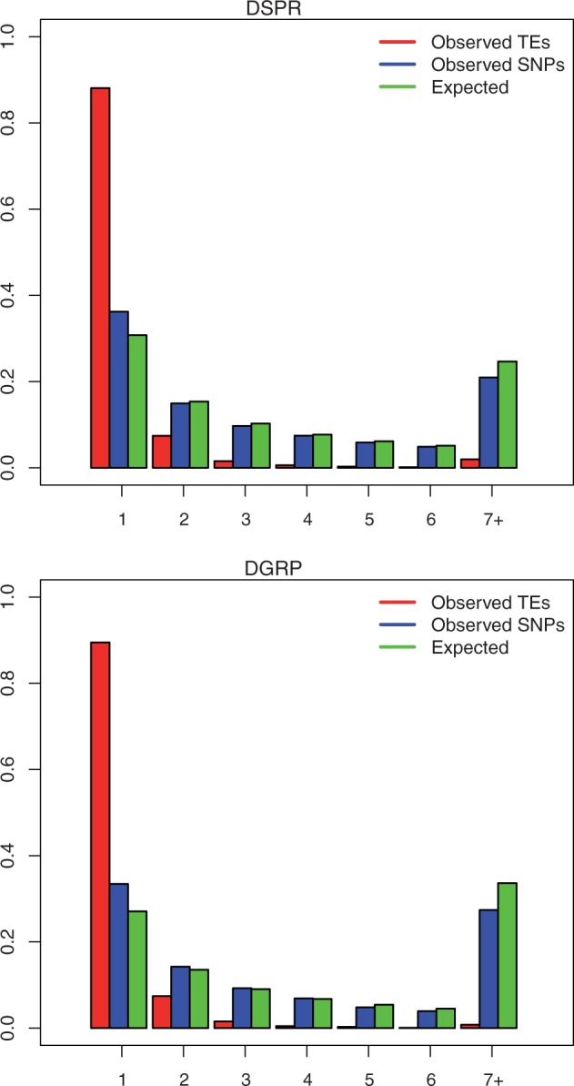
Derived allele count spectra for the DSRP lines and the DGRP25 lines where a positive presence or absence call was made for each insertion in each line, 6,613 insertions in the DSPR and 3,274 in the DGRP25. Count spectra for SNPs is from SNPs in introns ≤86 bp. χ² tests between observed and expected distributions result in P ≈ 0 for comparisons between TEs and the neutral model as well as between TEs and SNPs for both data sets.

Patterns of Transposable Element Insertions between Genes

For association studies, genotyping TE insertions within coding regions is of interest due to the potentially large effect of an insertion on gene function. A total of 2,931 genes (21.3% of annotated genes) had insertions in the DGRP resource. These are insertions which exist anywhere within the span of the gene from 5′ UTR to 3′ UTR. One thousand nine hundred fifteen genes, 13.9%, had insertions in the DSPR with 1,317 genes having insertions in both resources. The number of TE insertions within genes varied substantially between individual genes, up to a maximum of 78 insertions, though the majority of genes with insertions had only one insertion, 63.1% in the DSPR and 52.7% in the DGRP. The number and locations of individual insertions in a gene varied tremendously though the majority of insertions that fell within gene regions were in introns; 77.7% DSPR and 82.4% DGRP. TE number was strongly correlated with intron size (Pearson’s correlation coefficient = 0.79 for DSPR, 0.87 for DGRP, P ≈ 0 for both tests) (supplementary fig. S2, Supplementary Material online).

Examining the pattern of insertions in individual genes in the DSPR and DGRP data sets we found that RNA-binding protein 6 had the highest number of insertions, 62 in the DGRP lines and 21 in the DSPR lines. These insertions were typically unique to a single line though there were 3 insertions in more than one line in the DSPR and 14 insertions in more than one line in the DGRP.

Some genes accumulated many TE insertions, such as klarsicht (fig. 4A, gene images from the UCSC genome browser, Meyer et al. 2013) which had 29 total insertions. This gene also had a hotspot of insertions with seven independent insertions, each at low frequency, located within 3.6 kb of each other. Only one of these insertions was present in any given line and these could be functionally equivalent though independently arising mutations. Other genes had only a few insertions such as Notch (fig. 4B) and Delta (fig. 4C). The insertions in these genes were also at low frequency, and the few present were located in intronic regions.

Fig. 4.

Transposable element insertions in genes. The frequency above each insertion is the number of lines in which the element is present over the number of lines in which the element is validated as either present or absent. Gene images are from the UCSC genome browser (http://genome.ucsc.edu/, last accessed June 31, 2012).

While most insertions exist in only one panel some were found in both. Cyp6a20 (fig. 4D) contains a high frequency non-reference TE insertions present in both data sets, in 4 lines out of 121 lines where we were able to make a presence or absence call in the DGRP (hereafter shown as 4/121) and 3/14 lines in the DSPR. Both Cyp6a20 and klarsicht are examples of genes with TE insertions in exons, which was uncommon both in this data set and in previous studies (Kaminker et al. 2002; Lipatov et al. 2005).

Differences in the strength of selection against closely related genes can also be illustrated by patterns of TE insertions. The paralogs derailed (fig. 4F) and derailed-2 (fig. 4E) showed very different patterns of TE insertions, though the same pattern was seen in both resources. derailed-2, located on chromosome 2R, is in a region of moderate recombination, 1.99 cM/Mb, whereas derailed is located towards the distal end of 2L in a region of low recombination, 0.44 cM/Mb. Given the context of the recombination rates, the expectation would be that derailed would have a higher TE load since deleterious alleles are removed more efficiently in regions of high recombination (Hudson and Kaplan 1995), but the opposite pattern was observed.

While both genes play a role in Wnt5 signaling, mutations in derailed can cause major phenotypic changes in Drosophila nervous system development resulting in the loss of normal function (Yoshikawa et al. 2003). derailed-2, when mutated, produces only minor differences in neuron positioning (Sakurai et al. 2009). This suggests that either the strength of selection may be much higher against insertions in derailed or the insertion rates are unequal between the paralogs.

Gene Family Size and TEs

We used available information on gene families in Drosophila, Hahn et al. (2007) grouped into families based on sequence similarity, and found a very weak but significant effect of gene family size on the average number of TE insertions per kb in both resources (P value = 0.0003, R² = 0.001, DSPR; P value = 0.002, R² = 0.007 DGRP) (fig. 5A and B). Although there was a large variance in the number of insertions per kb in both resources (fig. 5A and B), the average number of TEs/kb increased as family size increased up to a moderately large family size.

Fig. 5.

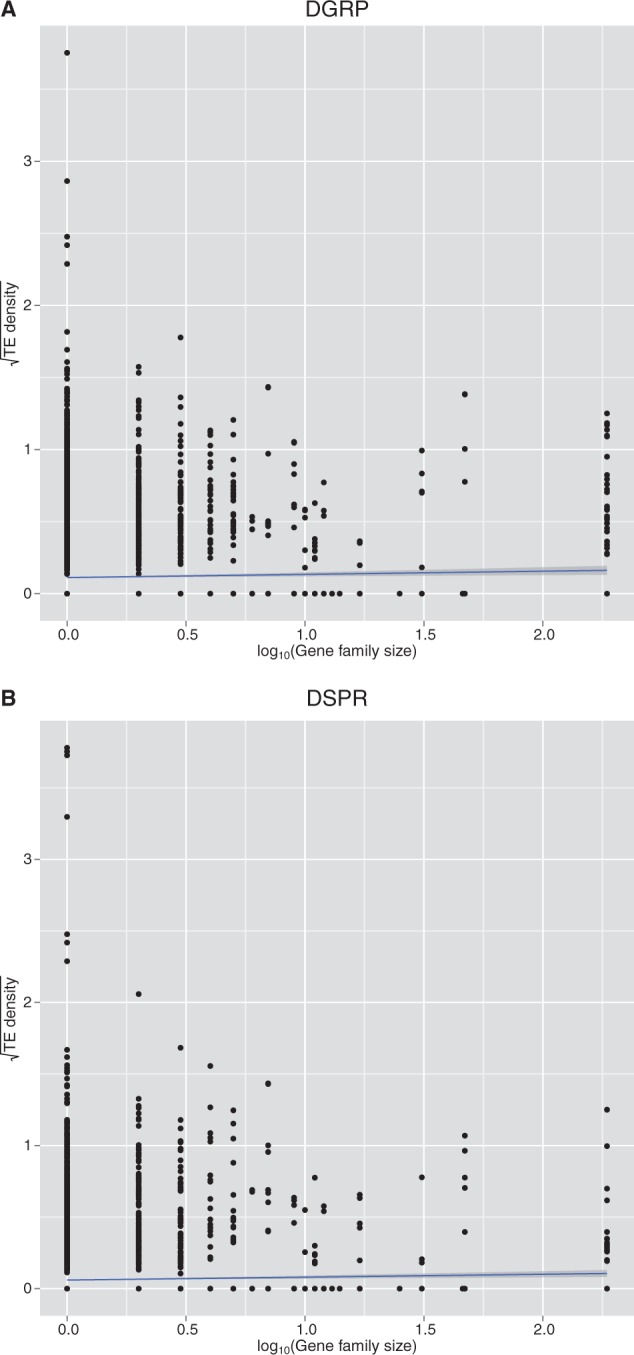
log₁₀(TE density) versus log₁₀(Gene family size).

Patterns of Variation between Resources

To replicate an association with a single causative allele, that allele must both exist in both panels and also be at high enough frequency to detect the association. Given that most TEs were singletons, and only 4.5% of insertion events were identified in both panels and were within genes, the replicability of associations with these alleles is likely to be low if alleles are considered individually. We examined shared insertions segregating at different frequencies between panels and found only two TE insertions in genes that were segregating at different frequencies in the DGRP versus DSPR resources, following Bonferroni correction (Fisher’s exact tests, P ≤ 0.00007). One of these was in an exon of both CG13175 and CG33964, a pair of overlapping genes. Here the TE insertion was at much higher frequency in the DGRP than in the DSPR (89/122 vs. 2/15). The other insertion was in an intron of Caliban and the frequency of this insertion was higher in the DSPR than the DGRP (11/15 vs. 7/116).

If insertions are considered as a class of mutation, then there may be better power to detect an association, assuming that different insertions contribute in the same way to the phenotype. We also examined genes with TE insertions (13.9% of genes), though not necessarily the same insertion in both resources. Treating all insertion alleles within a gene as equivalent, a comparison between resources showed that there were 21 genes which contain TEs at different frequencies between the DGRP versus DSPR, following Bonferroni correction (Fisher’s exact tests, P ≤ 0.000038197), including derailed-2 (supplementary table S6, Supplementary Material online).

Discussion

Distribution and Abundance of Transposable Elements

Previous work on transposable elements has generally been focused on a few families of TEs (Montgomery et al. 1987; Charlesworth and Lapid 1989; Charlesworth et al. 1992) or focused only on a single genome (Bartolome et al. 2002; Kaminker et al. 2002; Rizzon et al. 2002). We have presented a genomic analysis of TEs across a large number of lines and two data sets. We found that transposable elements in both resources are primarily found as singletons, with a few moderate to high frequency insertions. Transposable elements also segregated at lower allele frequencies than do presumed nonfunctional SNPs drawn from the same data set, suggesting that negative selection is acting upon TEs. However, there may be substantial variation in the age of transposable elements in different families, many LTR elements are thought to be young insertions (Bowen and McDonald 2001; Bergman and Bensasson 2007), while other families, like INE-1, are thought to be quite old (Kapitonov and Jurka 2003). This may create a situation where the young age of insertions is responsible for the excess of rare alleles. We found a non-random distribution of TE insertions across the genome, with increases of TEs in both the intergenic and intronic regions of the genome and decreases in exonic and UTR regions (Kaminker et al. 2002; Lipatov et al. 2005). Similar to previous studies, we found variation in TE density between chromosomes and higher densities of TEs in regions of low recombination (Charlesworth et al. 1994; Bartolome et al. 2002). We also found increased TE densities on the X relative to the autosomes, both in overall insertions and in some individual TE families (table 5).

Detection method and the size of the data set are likely to be contributing factors to differences between previous work and this study. Many previous studies have used in situ methods to ascertain TE number in samples and have looked at element accumulation at the base versus the midsections of chromosomes (Montgomery et al. 1987; Charlesworth et al. 1992) or have looked only at one genome (Bartolome et al. 2002; Rizzon et al. 2002). A previous PCR-based detection study found no difference in TE frequency between the X and the autosomes in natural populations (Petrov et al. 2011), but this study was biased in that it only looked at TEs shared with the reference sequence and thus did not capture the full picture of TEs in these populations.

While our analysis does disagree with previous work, these disagreements may be mainly due to the way in which regions of the genome are divided for examination. Rizzon et al. (2002) found an increase in copies of LTR retrotransposons on the X when they excluded pericentromeric, telomeric, and chromosome 4 from their analysis, though they found a deficit of TEs on the X when these regions are included. This finding is most directly comparable to our own finding for the entire TE data set since they exclude a very similar set of genomic regions. We do agree with previous work in our finding of higher densities of TEs in regions of low recombination than in high recombination (Charlesworth et al. 1994; Bartolome et al. 2002).

Examining individual element families, Carr et al. (2002) found an increase of mdg-3 elements and 297 elements on the X than would be expected under a random insertion model. Montgomery et al. (1987) found no evidence for a reduction in TEs on the X for both roo and 297 elements, but found fewer TEs on the X when looking at the 412 family. However, Charlesworth et al. (1992) observed the opposite pattern for roo and 297. Montgomery et al. (1991) also found that more roo elements in lab kept lines than they had previously observed in natural populations. We found significantly increased densities on the X for roo and significantly increased densities on the autosomes for 412.

Differences between previous studies of individual element families and our results may be due to a variety of reasons. First, we were able to annotate only about two-thirds of our TE insertions. This was primarily due to having insufficient sequence to reliably annotate the element or because independent annotation using sequence reconstructed from either end of the insertion did not yield the same element family annotation. This means that our density calculations for individual elements may be skewed by missing annotation information. Second, many previous studies (Montgomery et al. 1987; Charlesworth et al. 1992; Carr et al. 2002) examined only LTR elements. These elements are young (Bowen and McDonald 2001; Bergman and Bensasson 2007) and thus individual copies may not yet have been removed from the genome, thereby displaying different patterns of insertion than older, active elements.

What is clear is that there is great variability in TE density both within and between element families as well as within and between chromosomes. It may also be that the overall pattern is driven by a small group of families. In our data set INE-1 shows the largest pattern of difference between the X and autosomes, with an order of magnitude increase in mean TE density per line on the X over the autosomes, possibly due to an increased likelihood of fixation of insertions (Ometto et al. 2005), specifically on the X chromosome (Presgraves 2006). These INE-1 elements are a subset of the largest TE family in D. melanogaster, though only several dozen of them are in the euchromatin. INE-1 elements are also considered to be inactive in D. melanogaster and likely have not been mobile for >3 million years (Kapitonov and Jurka 2003). Consistent with this, most of the INE-1 elements we detected were fixed or nearly fixed in our data set. We did see some examples of low frequency insertions, which may be due to more recent transpositional events or incorrect TE annotation due to short sequences. The old age of INE-1 insertions also suggests that the extant elements are unlikely to be selected against. An increased density of TEs on the X compared with the autosomes suggests that it is not the fitness effects of insertions which govern TE copy number. Fitness effects would result in the more rapid removal of insertions on the X than insertions on the autosomes due to the increased selective pressures experienced on the X (Montgomery et al. 1987). Background selection also predicts that the X should be less burdened by deleterious recessives since it is hemizygous one third of the time (Charlesworth 1994).

However, it is unclear whether our observation of increased densities of TEs on the X relative to the autosomes fits with the ectopic exchange model. This model predicts that TEs will accumulate in regions of low ectopic exchange (Langley et al. 1988). The general assumption in the literature is that ectopic exchange is positively correlated with recombination rate (Langley et al. 1988; Montgomery et al. 1991). The X chromosome experiences higher levels of recombination than the autosomes, with an average of 3.6 cM/Mb for the X in regions of high recombination (cM/Mb > 2), whereas the autosomes have a mean of 3.36 cM/Mb. If recombination rate and ectopic exchange are positively correlated throughout the genome, then the expectation would be fewer TEs in the middle regions of the X where recombination rates are known to be high. This is the opposite of what we observe. If recombination rate and the rate of ectopic exchange are not positively correlated, then the ectopic exchange model may be correct, but data are lacking to properly address this issue. Currently, there are no direct measurements of the rate of ectopic exchange on a genome-wide scale in Drosophila during meiosis. Montgomery et al. (1991) observed little ectopic exchange between homozygous chromosomes in Drosophila melanogaster on the X chromosome in the region around the white locus. They also found that while recombination rate was reduced in both centromeric and telomeric regions, only the centromeric region displayed an increased density of TEs. This information is suggestive of differences between these regions in the rate of ectopic exchange.

The DGRP and DSPR are also composed of inbred lines which have been kept in laboratory conditions for some time, ∼9 years in the case of the DGRP lines and 40+ years in the case of the DSPR. Given that TE insertion mutations accumulate rapidly and in an increasing manner over time (Nuzhdin et al. 1997), the increased density of TEs on the X versus the autosomes may not be surprising if there is a higher transposition rate to the X. The only direct study to date focused on roo elements in D. melanogaster and did observe higher rates of insertion in the X than the autosomes (Vazquez et al. 2007).

Transposable Elements in Genes

The majority of genes, 81.3%, do not have any TE insertions in any line studied and intron length is a good predictor of the number of TEs within a gene. However, a few genes accumulate many insertions even after correcting for gene size and intron length and some genes have very few TEs even though they have large introns. The reasons why different genes may accumulate TE insertions may be quite different for individual genes. In some cases there may be hot spots for insertions, which, if insertions are neutral or only slightly deleterious, may result in large number of insertions in a small region. In other genes, the lack of TE accumulation may suggest selective pressures against TE accumulation.

Gene family size may also play a role in TE accumulation. We see an increase in TE density correlated with an increase in gene family size. This may indicate differences in selective pressures for genes in different sized families. Single-copy genes may experience more constraint, whereas in moderately sized gene families these constraints may be more relaxed, perhaps due to redundancy.

In the cytochrome p450 functional family of genes, we find that 37/89 of these genes have TE insertions, 25/89 in the DGRP, and 20/89 in the DSPR. Cytochrome p450 is also found to be in an enriched term in the DSPR for the set of genes containing TEs. The cytochrome p450 gene Cyp6g1 is known to confer resistance to DDT (Daborn et al. 2001) and TE-mediated copy number variation is associated with increasing resistance to DDT (Schmidt et al. 2010). This pattern of TE insertions in the DSPR may be reflective of the locations where DSPR lines were originally collected. The DSPR lines were gathered from various locations worldwide at a time when different pesticides were in use. The DGRP lines were gathered from a single geographic area in North America in 2003. Presumably these sets of lines have experienced different selective pressures with respect to pesticide resistance. In Cyp6a20 (fig. 4D), where TEs are segregating at different frequencies in the two resources, some similar effect may be occurring.

TE Detection Pipelines

The TE detection strategy used here is an improvement upon the strategy used in Mackay et al. (2012). The most notable differences between the data reported in Mackay et al. (2012) and the DGRP data reported here is substantial amount of new information. First, our pipeline improvements agree well with the previous implementation, with 81.2% of previous TE presence calls identified by the new pipeline. However, these calls represent on 18.2% of the presence calls made by the improved pipeline, demonstrating that we have identified significantly more calls than before. The incorporation of TE absence calls also allows us to provide a much more complete picture of TEs in euchromatic sequence in the DGRP.

The TE detection pipeline used here is similar to other pipelines which have been employed, but it is useful to describe briefly here the differences in approaches and why we followed the approach presented here. A useful discussion of common approaches to TE detection in many species can be found in Xing et al. (2013). One common method for TE detection is the split-read mapping approach which has been employed in Drosophila by Linheiro and Bergman (2012). This approach identifies TE insertions by locating individual sequence reads which span TE insertion breakpoints. This approach is the strategy of choice for next-generation sequencing experiments which produce only single-end reads. However, in a paired-end read situation, this approach may not take full advantage of the available data. Specifically, the size of window around the TE insertion breakpoint where informative reads can be found is governed by read length in a single-end experiment and fragment length in a paired-end experiment. Linheiro and Bergman (2012) discuss the importance of read length on TE detection and suggest that increased read length improves TE detection. In situations where read length is long and coverage is deep enough, the split-read method may be preferable to the paired-end detection strategy. However, for the data sets analyzed here, where read length is much shorter than fragment length, the paired-end detection strategy will capture more information.

The pipeline used here also has similarities to the pipeline used in Kofler et al. (2012). However, there are two major differences in these studies. First, Kofler et al. (2012) do not attempt to reconstruct their insertion breakpoints and second, the population studied by Kofler et al. (2012) was sequenced as a pool, rather than as individual lines. Because their pooled sequence data reflect on average less than 1× sequence coverage per line, Kofler et al. (2012) are primarily able to detect intermediate to high frequency TE insertions; their own analysis concludes that they cannot reliably detect insertions at frequency <7% (see supplementary fig. S2, Supplementary Material online, in their supplementary discussion). However, the literature to date (Charlesworth and Langley 1989; Charlesworth and Lapid 1989; Charlesworth et al. 1992) as well as the results of this study indicate that the majority of TEs in a population are found at very low frequency, often in only one individual in a population, and therefore beyond the scope of detection of Kofler et al. (2012).

Caveats

The D. melanogaster reference genome to which we aligned our data is a P-element-free genome. Therefore, the use of this reference will be biased against detecting any P elements existing in the data sets. In the case of the DSPR data set, this is not an issue since these lines are also all P-element-free (Macdonald and Long 2007). However, it is likely that the DGRP lines do harbor P elements. For the purpose of these analyses, we decided to ignore P elements and focus on the set of element families common to the two resources.

This situation does highlight the importance of having an appropriate reference sequence. To detect P elements in the genome of D. melanogaster, an artificially constructed reference sequence or a different assembled sequence containing the P element would need to be utilized. This also brings up the question about as yet undetected elements that exist at low frequency. If these elements do not have sufficient similarity to existing elements to be aligned to the reference genome, these elements will go undetected.

Conclusions

We have presented a description of transposable elements in two recently released QTL resources. Transposable elements can play important roles in gene function and regulation and incorporation of TE insertion information into any analysis performed with either of these two resources will present a more complete picture of genomic variation and its contribution to complex traits. In addition, it will be important for association studies attempting to replicate genotype–phenotype associations utilizing these resources to be aware of the potential contributions of TEs.

We have also demonstrated a next-generation, high-throughput sequencing analysis pipeline that is capable of detecting this type variation with a high rate of precision and specificity. We suggest that future studies using next-generation sequencing data utilize this technique.

Materials and Methods

Data Sets

Two data sets were used in this analysis. The first set consists of 131 inbred lines from the Drosophila Genetic Reference Panel (DGRP) (Mackay et al. 2012), SRA accession #SRP000694. The second set consists of 15 lines used to establish the Drosophila Synthetic Population Resource (DSPR) (King et al. 2012a) initially described in Macdonald and Long (2007), SRA accession #SRA051316. For the DGRP resource, both 454 and Illumina data were available, whereas only Illumina data are available for the DSPR. We utilized only the Illumina sequence data to ensure consistency in data collection across data sets. We calculated a mean coverage of 21× for the DGRP lines and 50× for the DSPR lines. Variation in coverage for the DGRP lines was substantial between lines, ranging from ∼4× average coverage to nearly 50× average coverage. We therefore dropped from the analysis four lines with an average coverage of 10× or less since low coverage can cause difficulties with assembly and TE identification. Sequence data for both data sets consisted of paired-end data with 54 bp reads for the DSPR and paired-end 100 bp reads, trimmed to 75 bp, for DGRP.

IBD in DGRP Data Set

We downloaded the SNP tables generated by the DGRP project from http://www.hgsc.bcm.tmc.edu/projects/dgrp/freeze1_July_2010/snp_calls/Illumina/ (last accessed July 30, 2010) to examine identity by descent in this data set. We performed an all by all comparison between lines examining sliding windows of 1 Mb across the genome with 100 kb steps between windows. We take a simple definition of IBD here. Whenever we identified two lines that were >95% identity at SNP positions in a 1 Mb region, we labeled the pair as IBD in the identified region and masked that region of the genome in the line with lower coverage. We also dropped entirely from our analysis any lines where >50% of the genome was determined to be IBD with other lines in the population (supplementary table S1, Supplementary Material online), removing from the analysis the line with lower average sequence coverage.

We modeled 1 Mb regions of 200 chromosomes in a coalescent simulation using the parameters theta = 0.01/site and 4Nr = 10*theta to determine the number of regions of ≥95% IBD under a Wright-Fisher population model using the MACS software (Chen et al. 2009). We simulated 1000 replicates of this simulation and tabulated the number of 1 Mb regions showing ≥95% IBD in each replicate.

Alignment

We aligned reads to the D. melanogaster reference genome (version 5.13 downloaded from FlyBase, flybase.org) using the aligner BWA (version 0.5.9, Li and Durbin 2009). We used the following parameters (aln -t 8 -l 13 -m 50000000 -R 5000) followed by the command “sampe” to resolve paired end mappings (using parameters -a 5000 -N 5000 -n 500). It is important when detecting TEs that the -R during the initial alignment and the -N parameter during the “sampe” phase be set high otherwise highly repetitive sequences that would be informative of the presence of a common element will be excluded from the data by the aligner. We also used the -I option for the DGRP lines, but not the DSPR, due to the differences in Illumina quality score output format as the two data sets were sequenced at different times. The -m parameter from the initial alignment step and the -n parameter from the paired-end resolution step deal with how BWA treats multiply aligning reads. An additional caveat is that some TE families, most notably the P-element family, is absent from the D. melanogaster reference sequence. Such families in the sequenced genomes will not align to the reference genome we used even if they are present in the sampled lines.

Transposable Element Detection

Transposable elements were detected by first identifying all reads that were aligned to an annotated TE in the reference genome (supplementary fig. S1, Supplementary Material online). We then identified the mates of these reads and selected only those mates which did not align to an annotated TE. These reads identify the set of read-pairs which span a TE insertion. The uniquely mapping, non-TE reads were then clustered based on their start position and chromosomal strand to identify putative TEs. Clusters on the plus strand were matched to clusters on the minus strand to produce pairs of clusters indicating either end of the putative TE. Once clusters were identified, we filtered out all events which contained fewer than three read-pairs consistent with a given insertion for each cluster. This means that putative events at this stage have a minimum of six read-pairs indicating the insertion, three on the plus strand and three on the minus strand.

We then extracted all reads and their mates that aligned to the identified regions of the genome and attempted to reconstruct the local area including the breakpoint of the TE. Because many TEs have repetitive regions at the ends of the element, we reconstructed the two breakpoints of the TE separately (see also supplementary fig. 23 from Mackay et al. 2012). Local reconstruction was done by running Phrap (version 1.090518, Ewing and Green 1998) with the following parameters (-forcelevel 10 -minscore 10 -minmatch 10). This set of parameters causes Phrap to do a Smith-Waterman comparison when it finds matches of at least 10 characters, but then relaxes the minimum alignment score and the final assembly parameters. This is necessary to reconstruct TEs because repetitive sequence within the TEs can result in a failure to reconstruct a contig if stricter assembly parameters are used. All code we developed for the detection of TEs will be freely available at www.molpopgen.org/Data/ (last accessed August 1, 2013).

Following reconstruction we used BlastN (verson 2.2.22) to compare reconstructed contigs to the D. melanogaster reference to confirm the presence of a TE. In most cases we were able to fully reconstruct both breakpoints of the TE. Fully reconstructed indicates that we could reconstruct a single contig which contained the breakpoint of the TE. In most cases the two breakpoints of the TE did not resolve to the same nucleotide, but instead identify the location of the target site duplication for the insertion (Linheiro and Bergman 2012, similar to fig. 1). These are cases where the upstream estimate of the breakpoint is slightly higher than the downstream estimate of the breakpoint and the difference in position can be seen as the likely span of the target site duplication. However, sometimes we were not able to fully reconstruct a contig, but instead generated two contigs; one containing uniquely aligning sequence and the other containing TE sequence. These contigs are known to belong together because reads forming one contig have their mates in the other contig. In these cases we have an approximate, but not precise, estimate of the TE breakpoint and are unable to identify the target site duplication.

After the first round of detection, we performed a second round of detection where we examined every location where a novel TE was detected in any line in all other lines. This included examining positions in one data set that were identified in the other data set. In addition we examined the locations of all known TEs in the D. melanogaster genome. For each location queried in each line, we extracted reads aligning to that location and their mates and used Phrap to reconstruct a contig. This allowed us to produce presence, absence, or missing data calls for all positions where TE was detected in all lines. The absence of a TE is determined by identifying reconstructed contigs that spanned the insertion position of the TE by at least 15 bp on either side. These absence calls were not included in Mackay et al. (2012). This also allows us to identify TEs that may be in regions of the genome with lower average sequence coverage compared with the rest of the genome provided that insertion is shared with another line where it was possible to detect the insertion.

Transposable Element Annotation

Annotation of novel TEs was performed by aligning reconstructed contigs with BlastN to the set of TEs found in the D. melanogaster reference. We chose the best match, based on overall length and BLAST reported e-value and called the novel TE a TE of that family. We also required a minimum of 80 bp of contig matching a TE to make an annotation call. This is an additional annotation analysis to the one we performed in Mackay et al. (2012). For each of the two contigs produced for each insertion, we determined the best match and then compared these to each other. TEs are classified as per the classification scheme put forth in Wicker et al. (2007). We annotated each TE insertion to the highest level of agreement between the two contigs; if the two contigs disagreed with each other at every level of classification, we called that element “undetermined”. This could result from nested insertions of elements where the 5′ end of the insertion is truly a different element from the 3′ end, or because the TE sequence is degraded and differs substantially from the reference sequence or because there was not enough TE sequence to meet our annotation guidelines. Because we can only reconstruct a maximum of few hundred bases at either end of the insertion, it is difficult to distinguish between these issues. We also did not attempt to determine the strand of the TE.

Validation

A subset of 190 TE insertion sites shared with the D. melanogaster reference were validated via PCR in a subset of nine of the DGRP lines by Blumenstiel JP, Chen X, He M, Bergman CM (unpublished data, http://arxiv.org/abs/1209.3456, last accessed June 26, 2013). To independently check IBD calls using SNP data, we also determined if pairs of lines were IBD for TEs in the same regions. In this comparison we only included TE insertions where both lines have a positive presence or absence call. This can also serve as a validation of our TE calling pipeline since if two segments are IBD they should share the same set of TEs.

Simulation

We selected a set of elements of different sizes and of TE classes from the set of TEs in the reference sequence and inserted them semi-randomly into the D. melanogaster reference genome in silico. Insertions were semi-random since we avoided areas already occupied by reference TEs and the centromeric and telomeric regions. Read pairs were then generated to construct fastq files. We then ran our TE detection pipeline as above through the initial annotation step. This process was repeated three times, to generate a simulation of 15×, 25×, and 50× coverage.

Recombination Rates

We wrote an R routine to estimate local recombination rates as a function of physical position. Briefly, we used “cyto-genetic-seq.tsv” from www.flybase.org (last accessed January 30, 2009) to assign a set of physical landmarks to genetic positions. For each chromosome arm we then fit a local polynomial relating cumulative cM to cumulative basepair (using locpoly). Unlike many prior local polynomial fits, we made the added assumption that this polynomial must be a monotonically increasing function (using monoproc); an assumption that is true for real data. We then fit a smooth spline to the above curve (using smooth.spline). The advantage of smooth.spline is that the resulting curves can be differentiated (and hence estimates of rates obtained directly). Finally, we fit a smooth spline to the first derivatives obtained from the prior smooth spline, largely to make the recombination rates less noisy near centromeres and telomeres. The R code is freely available at www.molpopgen.org/Data/ (last accessed August 1, 2013).

Data Set Restriction

Analyses performed on these data sets were restricted in two ways. First, we restricted our analyses to regions of the genome with low TE density and moderate recombination rates. We restricted our data set in this way because regions of high TE density make it more difficult to make accurate calls. Because our pipeline requires unique reads to positionally locate the TE insertion, regions with high TE density can lack enough unique sequence to generate these reads. The regions included in the analyses are X:300000–20800000, 2L:200000–20100000, 2R:2300000–21000000, 3L:100000–21900000, 3R:600000–27800000, which are not centromeric and telomeric regions. This excludes the majority of TEs annotated in the reference genome since these TEs are largely clustered together in centromeric regions. However, this does not affect our analysis since we are interested in TEs in the euchromatic portions of the genome.

Second, to restrict the set of reference TEs studied to full-length copies, we removed from the analysis all reference TEs that had a length that was less than 75% of the canonical annotated length of the TE. While these elements may still produce phenotypic effects, these elements are unlikely to be active copies. This reduced the number of reference TEs included in the analysis to 607 from 1085 TEs that are present in the reference genome in the regions included in our analysis.

Additionally some analyses were performed on the subset of 23 lines in the DGRP data set which had an average sequencing coverage of 25× or higher, hereafter referred to as DGRP25. This restriction was to mitigate the effect of differences in coverage between the two data sets. Simulations of transposable element detection via our pipeline, data not shown, indicate that TE detection at 25× is comparable to detection at 50×.

Site Count Spectra

We generated derived allele count spectra for TEs in the DSPR data set and the DGRP25 set of lines. We included only sites where we were able to make a positive presence or absence call for each line in the data set so that the number of lines was normalized for each resource for this analysis. Observed values were compared with expected values at counts 1, 2, 3, 4, 5, 6, and ≥7 under an infinite sites model via a χ² test. Categories 7 and higher were grouped due to low counts in some of these categories. We also calculated count spectra for SNPs present in small introns (introns ≤86 bp [Haddrill et al. 2005]), a group unlikely to have functional effects. We also used SoFoS, a site frequency rescaler (Hufford et al. 2012) to rescale the DSPR data set to the sample size of the DGRP25, from 15 to 23 samples, to see if the rescaled data show a different distribution of element counts from the observed DGRP25 data. We then did a Kolmogorov–Smirnov test to compare the two distributions as a test of different selective effects acting on the populations.

Genomic Context of TEs

Transposable elements were identified in regions of low (<2 cM/Mb) or high recombination (≥2 cM/Mb). FASTA files containing the annotated coordinates of 5′ UTRs, 3′ UTRs, intronic, intergenic, and full gene span regions for version 5.13 of the D. melanogaster reference were downloaded from flybase (www.flybase.org, last accessed January 30, 2009). Version 5.13 of the reference annotation was used for comparative purposes with the DGRP analysis (Mackay et al. 2012). Because alternative transcripts can result in the same genomic position being classified in multiple categories, we labeled each TE as every appropriate category. This occurred with 5.2% of TEs in the DGRP and 6.0% of TEs in the DSPR. When calculating the percentage of the reference genome in our restricted areas of analysis that were classified as each genomic type, we followed the same strategy.

We compared our observations of TE insertions to a binomial distribution, to determine whether TEs were distributed randomly throughout the genome. We used the pbinom function in R (R Development Core Team 2008) setting the number of trials to the total number of TE insertion locations in the data set and the probability of success to the proportion of the genome defined as each context (intron, exon, 3′ UTR, 5′ UTR, or intergenic). We did one tailed tests in each case. For exon, 3′ UTR, and 5′ UTR tests, we calculated the probability of observing the observed value or fewer TEs. For intron and intergenic tests, we calculated the probability of observing the observed value or more TEs.

Variables Affecting TE Density

For the DGRP25 and DSPR data sets, we calculated TE density in terms of TEs/Mb. For this analysis we also excluded chromosome 4. We examined the effects of recombination rate, chromosome, and TE element family on TE density using the standard linear model in R. We used the lm() function to define our model as follows: TEs/Mb ∼ Line + Recombination Rate + Chromosome + Recombination Rate * Chromosome. We performed this analysis both for the set of all TEs and also for 15 TE families with moderate to high number of copies in our data set (supplementary table S4, Supplementary Material online). We selected individual TE families for this additional analysis based on their level of abundance in the data sets and their having been previously studied by Montgomery et al. (1987) and Bartolome et al. (2002).

Gene Families

We downloaded the Dfam database from (http://www.indiana.edu/∼hahnlab/fly/DfamDB/drosophila_frb.html, last accessed September 1, 2012). This database describes all members of all gene families clustered using a fuzzy reciprocal BLAST method as described in Hahn et al. (2007) for 12 Drosophila species. We used R to perform a linear regression using a simple model where the square root (TE density) in a gene is the random variable and log₁₀ (gene family size) is the independent variable.

Variation between Resources

For each TE present in both data sets, we compared the frequency of the TE in each population using Fisher’s exact test. We excluded from this analysis all insertions where we were unable to make a presence/absence call in at least 100 of the DGRP lines or 13 of the DSPR lines. For each gene with TE insertions in both data sets, we compared the frequency at which the gene contains TEs between data sets using a Fisher’s exact test.

Supplementary Material

Supplementary tables S1–S6 and figures S1 and S2 are available at Molecular Biology and Evolution online (http://www.mbe.oxfordjournals.org/).

References

- Altschul SF, Gish W, Miller W, Myers EW, Lipman DJ. Basic local alignment search tool. J Mol Biol. 1990;215:403–410. doi: 10.1016/S0022-2836(05)80360-2. [DOI] [PubMed] [Google Scholar]
- Aminetzach YT, Macpherson JM, Petrov DA. Pesticide resistance via transposition-mediated adaptive gene truncation in Drosophila. Science. 2005;309:764–767. doi: 10.1126/science.1112699. [DOI] [PubMed] [Google Scholar]
- Bartolome C, Maside X, Charlesworth B. On the abundance and distribution of transposable elements in the genome of Drosophila melanogaster. Mol Biol Evol. 2002;19:926–937. doi: 10.1093/oxfordjournals.molbev.a004150. [DOI] [PubMed] [Google Scholar]
- Bennetzen JL. Transposable element contributions to plant gene and genome evolution. Plant Mol Biol. 2000;42:251–269. [PubMed] [Google Scholar]
- Bergman CM, Bensasson D. Recent LTR retrotransposon insertion contrasts with waves of non-LTR insertion since speciation in Drosophila melanogaster. Proc Natl Acad Sci U S A. 2007;104:11340–11345. doi: 10.1073/pnas.0702552104. [DOI] [PMC free article] [PubMed] [Google Scholar]
- Biemont C, Vieira C. Junk DNA as an evolutionary force. Nature. 2006;443:521–524. doi: 10.1038/443521a. [DOI] [PubMed] [Google Scholar]
- Birchler JA, Hiebert JC. Interaction of the Enhancer of white-apricot with transposable element alleles at the white locus in Drosophila melanogaster. Genetics. 1989;122:129–138. doi: 10.1093/genetics/122.1.129. [DOI] [PMC free article] [PubMed] [Google Scholar]
- Birchler JA, Hiebert JC, Rabinow L. Interaction of the mottler of white with transposable element alleles at the white locus in Drosophila melanogaster. Genes Dev. 1989;3:73–84. doi: 10.1101/gad.3.1.73. [DOI] [PubMed] [Google Scholar]
- Bowen NJ, McDonald JF. Drosophila euchromatic LTR retrotransposons are much younger than the host species in which they reside. Genome Res. 2001;11:1527–1540. doi: 10.1101/gr.164201. [DOI] [PMC free article] [PubMed] [Google Scholar]
- Carr M, Soloway JR, Robinson TE, Brookfield JF. Mechanisms regulating copy numbers of six LTR retrotransposons in the genome of Drosophila melanogaster. Chromosoma. 2002;110:511–518. doi: 10.1007/s00412-001-0174-0. [DOI] [PubMed] [Google Scholar]
- Charlesworth B. The effect of background selection against deleterious mutations on weakly selected linked variants. Genet Res. 1994;63:213–227. doi: 10.1017/s0016672300032365. [DOI] [PubMed] [Google Scholar]
- Charlesworth B, Jarne P, Assimacopoulos S. The distribution of transposable elements within and between chromosomes in a population of Drosophila melanogaster. III. Element abundances in heterochromatin. Genet Res. 1994;64:183–197. doi: 10.1017/s0016672300032845. [DOI] [PubMed] [Google Scholar]
- Charlesworth B, Langley CH. The population genetics of Drosophila transposable elements. Annu Rev Genet. 1989;23:251–287. doi: 10.1146/annurev.ge.23.120189.001343. [DOI] [PubMed] [Google Scholar]
- Charlesworth B, Lapid A. A study of ten families of transposable elements on X chromosomes from a population of Drosophila melanogaster. Genet Res. 1989;54:113–125. doi: 10.1017/s0016672300028482. [DOI] [PubMed] [Google Scholar]
- Charlesworth B, Lapid A, Canada D. The distribution of transposable elements within and between chromosomes in a population of Drosophila melanogaster. I. Element frequencies and distribution. Genet Res. 1992;60:103–114. doi: 10.1017/s0016672300030792. [DOI] [PubMed] [Google Scholar]
- Chen GK, Marjoram P, Wall JD. Fast and flexible simulation of DNA sequence data. Genome Res. 2009;19:136–142. doi: 10.1101/gr.083634.108. [DOI] [PMC free article] [PubMed] [Google Scholar]
- Chung H, Bogwitz MR, McCart C, Andrianopoulos A, Ffrench-Constant RH, Batterham P, Daborn PJ. Cis-regulatory elements in the accord retrotransposon result in tissue-specific expression of the Drosophila melanogaster insecticide resistance gene Cyp6g1. Genetics. 2007;175:1071–1077. doi: 10.1534/genetics.106.066597. [DOI] [PMC free article] [PubMed] [Google Scholar]
- Cutter AD, Good JM, Pappas CT, Saunders MA, Starrett DM, Wheeler TJ. Transposable element orientation bias in the Drosophila melanogaster genome. J Mol Evol. 2005;6:733–741. doi: 10.1007/s00239-004-0243-0. [DOI] [PubMed] [Google Scholar]
- Daborn P, Boundy S, Yen J, Pittendrigh B, Ffrench-Constant R. DDT resistance in Drosophila correlates with Cyp6g1 over-expression and confers cross-resistance to the neonicotinoid imidacloprid. Mol Genet Genomics. 2001;266:556–563. doi: 10.1007/s004380100531. [DOI] [PubMed] [Google Scholar]
- Deloger M, Cavalli FMG, Lerat E, Biemont C, Sagot M-F, Vieira C. Identification of expressed transposable element insertions in the sequenced genome of Drosophila melanogaster. Gene. 2009;439:55–62. doi: 10.1016/j.gene.2009.03.015. [DOI] [PubMed] [Google Scholar]
- Dworkin I, Palsson A, Gibson G. Replication of an Egfr-wing shape association in a wild-caught cohort of Drosophila melanogaster. Genetics. 2005;169:2115–2125. doi: 10.1534/genetics.104.035766. [DOI] [PMC free article] [PubMed] [Google Scholar]
- Ewing B, Green P. Base-calling of automated sequencer traces using Phred. II. Error probabilities. Genome Res. 1998;8:186–194. [PubMed] [Google Scholar]
- Gruber JD, Genissel A, Macdonald SJ, Long AD. How repeatable are associations between polymorphisms in achaete-scute and bristle number variation in Drosophila. Genetics. 2007;175:1987–1997. doi: 10.1534/genetics.106.067108. [DOI] [PMC free article] [PubMed] [Google Scholar]
- Haddrill PR, Charlesworth B, Halligan DL, Andolfatto P. Patterns of intron sequence evolution in Drosophila are dependent upon length and GC content. Genome Biol. 2005;6:R67. doi: 10.1186/gb-2005-6-8-r67. [DOI] [PMC free article] [PubMed] [Google Scholar]
- Hahn MW, Han MV, Han S-G. Gene family evolution across 12 Drosophila genomes. PLoS Genet. 2007;3:e197. doi: 10.1371/journal.pgen.0030197. [DOI] [PMC free article] [PubMed] [Google Scholar]
- Hirschhorn JN, Daly MJ. Genome-wide association studies for common diseases and complex traits. Nat Rev Genet. 2005;6:95–108. doi: 10.1038/nrg1521. [DOI] [PubMed] [Google Scholar]
- Hudson RR, Kaplan NL. Deleterious background selection with recombination. Genetics. 1995;141:1605–1617. doi: 10.1093/genetics/141.4.1605. [DOI] [PMC free article] [PubMed] [Google Scholar]
- Hufford MB, Xu X, van Heerwaarden J, et al. (25 co-authors) Comparative population genomics of maize domestication and improvement. Nat Genet. 2012;44:808–811. doi: 10.1038/ng.2309. [DOI] [PMC free article] [PubMed] [Google Scholar]
- Kaminker JS, Bergman CM, Kronmiller B, et al. (12 co-authors) The transposable elements of the Drosophila melanogaster euchromatin: a genomics perspective. Genome Biol. 2002;3 doi: 10.1186/gb-2002-3-12-research0084. RESEARCH0084. [DOI] [PMC free article] [PubMed] [Google Scholar]
- Kapitonov VV, Jurka J. Molecular paleontology of transposable elements in the Drosophila melanogaster genome. Proc Natl Acad Sci U S A. 2003;100:6569–6574. doi: 10.1073/pnas.0732024100. [DOI] [PMC free article] [PubMed] [Google Scholar]
- Kazazian HH. Mobile elements: drivers of genome evolution. Science. 2004;303:1626–1632. doi: 10.1126/science.1089670. [DOI] [PubMed] [Google Scholar]
- Kidwell MG. Transposable elements and the evolution of genome size in eukaryotes. Genetica. 2002;115:49–63. doi: 10.1023/a:1016072014259. [DOI] [PubMed] [Google Scholar]
- King EG, Macdonald SJ, Long AD. Properties and power of the Drosophila synthetic population resource for the routine dissection of complex traits. Genetics. 2012a;191:935–949. doi: 10.1534/genetics.112.138537. [DOI] [PMC free article] [PubMed] [Google Scholar]
- King EG, Merkes CM, McNeil CL, Hoofer SR, Sen S, Broman KW, Long AD, Macdonald SJ. Genetic dissection of a model complex trait using the Drosophila synthetic population resource. Genome Res. 2012b;22:1558–1566. doi: 10.1101/gr.134031.111. [DOI] [PMC free article] [PubMed] [Google Scholar]
- Kofler R, Betancourt AJ, Schlotterer C. Sequencing of pooled DNA samples (Pool-Seq) uncovers complex dynamics of transposable element insertions in Drosophila melanogaster. PLoS Genet. 2012;8:e1002487. doi: 10.1371/journal.pgen.1002487. [DOI] [PMC free article] [PubMed] [Google Scholar]
- Langley CH, Montgomery E, Hudson R, Kaplan N, Charlesworth B. On the role of unequal exchange in the containment of transposable element copy number. Genet Res. 1988;52:223–235. doi: 10.1017/s0016672300027695. [DOI] [PubMed] [Google Scholar]
- Li H, Durbin R. Fast and accurate short read alignment with Burrows-Wheeler transform. Bioinformatics. 2009;25:1754–1760. doi: 10.1093/bioinformatics/btp324. [DOI] [PMC free article] [PubMed] [Google Scholar]
- Linheiro RS, Bergman CM. Whole genome resequencing reveals natural target site preferences of transposable elements in Drosophila melanogaster. PLoS One. 2012;7:e30008. doi: 10.1371/journal.pone.0030008. [DOI] [PMC free article] [PubMed] [Google Scholar]
- Lipatov M, Lenkov L, Petrov DA, Bergman CM. Paucity of chimeric gene-transposable elements in the Drosophila melanogaster genome. BMC Biol. 2005;3:24. doi: 10.1186/1741-7007-3-24. [DOI] [PMC free article] [PubMed] [Google Scholar]
- Long AD, Lyman RF, Morgan AH, Langley CH, Mackay TFC. Both naturally occurring insertions of transposable elements and intermediate frequency polymorphisms at the achaete-scute complex are associated with bristle number in Drosophila melanogaster. Genetics. 2000;154:1255–1269. doi: 10.1093/genetics/154.3.1255. [DOI] [PMC free article] [PubMed] [Google Scholar]
- Lonnig W-E, Saedler H. Chromosome rearrangements and transposable elements. Annu Rev Genet. 2002;36:389–410. doi: 10.1146/annurev.genet.36.040202.092802. [DOI] [PubMed] [Google Scholar]
- Macdonald SJ, Long AD. Joint estimates of quantitative trait locus effect and frequency using synthetic recombinant populations of Drosophila melanogaster. Genetics. 2007;176:1261–1281. doi: 10.1534/genetics.106.069641. [DOI] [PMC free article] [PubMed] [Google Scholar]
- Macdonald SJ, Pastinen T, Long AD. The effect of polymorphisms in the Enhancer of split gene complex on bristle number variation in a large wild-caught cohort of Drosophila melanogaster. Genetics. 2005;171:1741–1756. doi: 10.1534/genetics.105.045344. [DOI] [PMC free article] [PubMed] [Google Scholar]
- Mackay TFC. Jumping genes meet abdominal bristles: hybrid dysgenesis-induced quantitative variation in Drosophila melanogaster. Genet Res. 1984;44:231–237. [Google Scholar]
- Mackay TFC. Transposable elements and fitness in Drosophila melanogaster. Genome. 1989;31:284–295. doi: 10.1139/g89-046. [DOI] [PubMed] [Google Scholar]
- Mackay TFC. Mutations and quantitative genetic variation: lessons from Drosophila. Philos Trans R Soc Lond B Biol Sci. 2010;365:1229–1239. doi: 10.1098/rstb.2009.0315. [DOI] [PMC free article] [PubMed] [Google Scholar]
- Mackay TFC, Langley CH. Molecular and phenotypic variation in the achaete-scute region of Drosophila melanogaster. Nature. 1990;348:64–66. doi: 10.1038/348064a0. [DOI] [PubMed] [Google Scholar]
- Mackay TFC, Lyman RF, Jackson MS. Effects of P element insertions on quantitative traits in Drosophila melanogaster. Genetics. 1992;130:315–332. doi: 10.1093/genetics/130.2.315. [DOI] [PMC free article] [PubMed] [Google Scholar]
- Mackay TFC, Richards S, Stone EA, et al. (52 co-authors) The Drosophila melanogaster genetic reference panel. Nature. 2012;482:173–178. doi: 10.1038/nature10811. [DOI] [PMC free article] [PubMed] [Google Scholar]
- Meyer LR, Zweig AS, Hinrichs AS, et al. (32 co-authors) The UCSC genome browser database: extensions and updates 2013. Nucleic Acids Res. 2013;41:D64–D69. doi: 10.1093/nar/gks1048. [DOI] [PMC free article] [PubMed] [Google Scholar]
- Montgomery E, Charlesworth B, Langley CH. A test for the role of natural selection in the stabilization of transposable element copy number in a population of Drosophila melanogaster. Genet Res. 1987;49:31–41. doi: 10.1017/s0016672300026707. [DOI] [PubMed] [Google Scholar]
- Montgomery EA, Huang S-M, Langley CH, Judd BH. Chromosome rearrangement by ectopic recombination in Drosophila melanogaster: genome structure and evolution. Genetics. 1991;129:1085–1098. doi: 10.1093/genetics/129.4.1085. [DOI] [PMC free article] [PubMed] [Google Scholar]
- NCI-NHGRI Working Group on Replication in Association Studies. Replicating genotype-phenotype associations. Nature. 2007;447:655–660. doi: 10.1038/447655a. [DOI] [PubMed] [Google Scholar]
- Nuzhdin SV, Mackay TFC. The genomic rate of transposable element movement in Drosophila melanogaster. Mol Biol Evol. 1994;12:180–181. doi: 10.1093/oxfordjournals.molbev.a040188. [DOI] [PubMed] [Google Scholar]
- Nuzhdin SV, Pasyukova EG, Mackay TFC. Accumulation of transposable elements in laboratory lines of Drosophila melanogaster. Genetica. 1997;100:167–175. [PubMed] [Google Scholar]
- Ometto L, Stephan W, Lorenzo DD. Insertion/deletion and nucleotide polymorphism data reveal constraints in Drosophila melanogaster introns and intergenic regions. Genetics. 2005;169:1521–1527. doi: 10.1534/genetics.104.037689. [DOI] [PMC free article] [PubMed] [Google Scholar]
- Palsson A, Gibson G. Association between nucleotide variation in Egfr and wing shape in Drosophila melanogaster. Genetics. 2004;167:1187–1198. doi: 10.1534/genetics.103.021766. [DOI] [PMC free article] [PubMed] [Google Scholar]
- Petrov DA, Fiston-Lavier A-S, Lipatov M, Lenkov K, Gonzalez J. Population genomics of transposable elements in Drosophila melanogaster. Mol Biol Evol. 2011;28:1633–1644. doi: 10.1093/molbev/msq337. [DOI] [PMC free article] [PubMed] [Google Scholar]
- Presgraves DC. Intron length evolution in Drosophila. Mol Biol Evol. 2006;13:2203–2213. doi: 10.1093/molbev/msl094. [DOI] [PubMed] [Google Scholar]
- Quinian AR, Hall IM. BEDTools: a flexible suite of utilities for comparing genomic features. Bioinformatics. 2010;26:841–842. doi: 10.1093/bioinformatics/btq033. [DOI] [PMC free article] [PubMed] [Google Scholar]
- R Development Core Team. R: a language and environment for statistical computing. Vienna Austria: R Foundation for Statistical Computing; 2008. [cited 2013 May 1] Available from: http://www.R-project.org. [Google Scholar]
- Rizzon C, Marais G, Gouy M, Biemont C. Recombination rate and the distribution of transposable elements in the Drosophila melanogaster genome. Genome Res. 2002;12:400–407. doi: 10.1101/gr.210802. [DOI] [PMC free article] [PubMed] [Google Scholar]
- Sackton TB, Kulathinal RJ, Bergman CM, Quinlan AR, Dopman EB, Carneiro M, Marth GT, Hartl DL, Clark AG. Population genomic inferences from sparse high-throughput sequencing of two populations of Drosophila melanogaster. Genome Biol Evol. 2009;1:449–465. doi: 10.1093/gbe/evp048. [DOI] [PMC free article] [PubMed] [Google Scholar]
- Sakurai M, Aoki T, Yoshikawa S, et al. (11 co-authors) Differentially expressed Drl and Drl-2 play opposing roles in Wnt5 signaling during Drosophila olfactory system development. J Neurosci. 2009;29:4972–4980. doi: 10.1523/JNEUROSCI.2821-08.2009. [DOI] [PMC free article] [PubMed] [Google Scholar]
- Schmidt JM, Good RT, Appleton B, et al. (11 co-authors) Copy number variation and transposable elements feature in recent, ongoing adaptation at the Cyp6g1 locus. PLoS Genet. 2010;6:e1000998. doi: 10.1371/journal.pgen.1000998. [DOI] [PMC free article] [PubMed] [Google Scholar]
- Shrimpton AE, Mackay TFC, Brown AJL. Transposable element-induced response to artificial selection in Drosophila melanogaster: molecular analysis of selection lines. Genetics. 1990;125:803–811. doi: 10.1093/genetics/125.4.803. [DOI] [PMC free article] [PubMed] [Google Scholar]
- Slotkin RK, Martienssen R. Transposable elements and the epigenetic regulation of the genome. Nat Rev Genet. 2007;8:272–285. doi: 10.1038/nrg2072. [DOI] [PubMed] [Google Scholar]
- Smith PA, Corces VG. Drosophila transposable elements: mechanisms of mutagenesis and interactions with the host genome. Adv Genet. 1991;29:229–300. doi: 10.1016/s0065-2660(08)60109-1. [DOI] [PubMed] [Google Scholar]
- Thornton K. Libsequence; a C++ class library for evolutionary genetic analysis. Bioinformatics. 2003;19:2325–2327. doi: 10.1093/bioinformatics/btg316. [DOI] [PubMed] [Google Scholar]
- Vazquez JF, Albornoz J, Dominguez A. Direct determination of the effects of genotype and extreme temperature on the transposition of roo in long-term mutation accumulation lines of Drosophila melanogaster. Mol Genet Genomics. 2007;278:653–664. doi: 10.1007/s00438-007-0282-5. [DOI] [PubMed] [Google Scholar]
- Voight BF, Pritchard JK. Confounding from cryptic relatedness in case-control association studies. PLoS Genet. 2005;1:e32. doi: 10.1371/journal.pgen.0010032. [DOI] [PMC free article] [PubMed] [Google Scholar]
- Wakeley J. Coalescent theory: an introduction. Greenwood Village: Roberts and Company Publishers; 2009. [Google Scholar]
- Wicker T, Sabot F, Hua-Van A, et al. (13 co-authors) A unified classification system for eukaryotic transposable elements. Nat Rev Genet. 2007;8:973–982. doi: 10.1038/nrg2165. [DOI] [PubMed] [Google Scholar]
- Xing J, Witherspoon DJ, Jorde LB. Mobile element biology: new possibilities with high-throughput sequencing. Trends Genet. 2013;29:280–289. doi: 10.1016/j.tig.2012.12.002. [DOI] [PMC free article] [PubMed] [Google Scholar]
- Yoshikawa S, McKinnon RD, Kokel M, Thomas JB. Wnt-mediated axon guidance via Drosophila derailed receptor. Nature. 2003;422:583–588. doi: 10.1038/nature01522. [DOI] [PubMed] [Google Scholar]
- Zachar Z, Bingham PM. Regulation of white locus expression: the structure of mutant alleles at the white locus of Drosophila melanogaster. Cell. 1982;30:529–541. doi: 10.1016/0092-8674(82)90250-1. [DOI] [PubMed] [Google Scholar]
Associated Data
This section collects any data citations, data availability statements, or supplementary materials included in this article.