Assessing the component associations of the healthy worker survivor bias: occupational asbestos exposure and lung cancer mortality

Abstract

Background

The healthy worker survivor bias is well-recognized in occupational epidemiology. Three component associations are necessary for this bias to occur: i) prior exposure and employment status; ii) employment status and subsequent exposure; and iii) employment status and mortality. Together, these associations result in time-varying confounding affected by prior exposure. We illustrate how these associations can be assessed using standard regression methods.

Method

We use data from 2975 asbestos textile factory workers hired between January 1940 and December 1965 and followed for lung cancer mortality through December 2001.

Results

At entry, median age was 24 years, with 42% female and 19% non-Caucasian. Over follow-up, 21% and 17% of person-years were classified as at work and exposed to any asbestos, respectively. For a 100 fiber-year/mL increase in cumulative asbestos, the covariate-adjusted hazard of leaving work decreased by 52% (95% confidence interval [CI], 46–58). The association between employment status and subsequent asbestos exposure was strong due to nonpositivity: 88.3% of person-years at work (95% CI, 87.0–89.5) were classified as exposed to any asbestos; no person-years were classified as exposed to asbestos after leaving work. Finally, leaving active employment was associated with a 48% (95% CI, 9–71) decrease in the covariate-adjusted hazard of lung cancer mortality.

Conclusions

We found strong associations for the components of the healthy worker survivor bias in these data. Standard methods, which fail to properly account for time-varying confounding affected by prior exposure, may provide biased estimates of the effect of asbestos on lung cancer mortality under these conditions.

Introduction

The goal of an occupational epidemiologic study is often to estimate the effect of a work-based exposure on a health-related outcome. The healthy worker survivor bias has long been known to potentially threaten the validity of such effect estimates [1]. Causal diagrams [2] have recently been used to define the healthy worker survivor bias as an example of time-varying confounding affected by prior exposure (henceforth, time-varying confounding) [3]. With causal diagrams, three component associations of the healthy worker survivor bias can be identified (Fig. 1). Component 1 is the association between prior exposure and employment status. Component 2 is the association between employment status and subsequent exposure. Component 3 is the association between employment status and survival. The severity of the healthy worker survivor bias depends on the magnitude of these three component associations [4].

Fig. 1.

Causal diagram representing the healthy worker survivor bias. Let j be index age, A represent continuous asbestos exposure cumulated over follow-up, X represent continuous asbestos exposure, W index employment status, U a common cause of W and T, and T index survival time. C1 = component 1; C2 = component 2; C3 = component 3.

If all three of these component associations are present, standard methods may yield biased estimates of the exposure–outcome relationship: Adjusting for employment status may result in an exposure–outcome effect estimate that is subject to collider stratification bias [5]; however, not adjusting for employment status may yield a confounded exposure–outcome effect estimate. Moreover, individuals who leave work have no chance of incurring work-based exposure at subsequent time points. Consequently, adjusting for employment status may result in a violation of the positivity assumption (or nonpositivity) [3,4], which requires exposed and unexposed individuals in all confounder strata at all time points [6–8]. When positivity does not hold, an inference made regarding an exposure–outcome relation is (by definition) not fully supported by the data [7]. Violations of the positivity assumption (nonpositivity) are of two kinds: Random and systematic. Random nonpositivity occurs when no individuals happen to be observed within one or more confounder strata. However, the healthy worker survivor effect is an example of systematic nonpositivity, in which individuals who have terminated active employment cannot be exposed. By definition, nonpositivity guarantees that an association exists between two variables. In an occupational cohort study, systematic nonpositivity between employment status and the exposure jeopardizes the identifiability of the causal effect of the exposure on the outcome of interest [9]. Although both types of nonpositivity can result in a nonidentifiable effect estimate, as a structural feature of the scenario under study, systematic nonpositivity is of greater concern [4].

The parametric g-formula [10–12] and g-estimation of structural nested models [12–14] are two analytic strategies that have been developed to account for time-varying confounding affected by prior exposure. Unlike standard methods, g-methods yield consistent estimates of the effect of exposure on the outcome when each of the three component associations is present. However, specialized knowledge and tailored computer code is needed to implement these methods. Thus, before undertaking an analysis using these methods, researchers can assess the component associations of the healthy worker survivor bias as a simple diagnostic to determine whether such methods are required. In this paper, we assess the component associations of the healthy worker survivor bias in a cohort of 2975 asbestos textile factory workers followed for lung cancer mortality between 1940 and 2001 in the southern United States.

Methods

Study cohort

The South Carolina Chrysotile Asbestos study is an occupational cohort study of the relationship between workplace asbestos exposure and lung cancer mortality over a 60-year period. The cohort consisted of 3072 individuals who worked in an asbestos textile factory for 6 months or more with at least 1 month of employment between January 1, 1940 and December 31, 1965 [15]. We excluded 97 individuals (3%) who left work before 18 years of age to ensure adequately sized early age risk sets, leaving a final sample of 2975 individuals. Follow-up started on January 1, 1940. Workers were followed for vital status and cause of death until loss to follow-up or administrative censoring on December 31, 2001. Date of birth, gender, and race (Caucasian versus non-Caucasian) were ascertained from company personnel records. This study was conducted on de-identified existing records and therefore deemed not human subjects research.

Mortality ascertainment

The primary outcome, here and in many studies of asbestos exposure, is lung cancer mortality. Mortality dates were obtained by National Death Index (NDI), with lung cancer defined by the appropriate International Classification of Diseases codes (see Appendix 1 for details).

Asbestos exposure assessment

Asbestos exposure levels were assigned using a job-exposure matrix. Following previous research [16–21], annual exposure levels, in fiber-years per milliliter, were calculated as the product of duration of exposure in that calendar year and the department, task, and calendar period–specific average concentration of chrysotile fibers longer than 5 µm/mL air to which an individual was exposed (see Appendix 2 for details).

Notation and causal structure

Causal diagrams [2] can be used to graphically represent and identify sources of bias in an exposure-outcome effect estimate (see Glymour et al. [22] for a detailed introduction, and Robins and Hernán [12] section 23.7 for a more advanced treatment). Figure 1 is a causal diagram illustrating the healthy worker survivor bias [3].

The graph should be read from left to right, indicating the passage of time. For an observation at age j, we let A(j) denote a chosen summary metric of asbestos exposure history such as the cumulative exposure accrued up to age j. We let X(j) denote an estimate of the asbestos exposure in fiber-years per milliliter accrued during age j [i.e., during the interval [j,j + 1)]. We define an indicator of leaving active employment, denoted W(j), as a binary variable equal to 1 if the in dividual was not actively employed at the asbestos textile factory under study at all during age j. For example, for an individual who left employment mid-year at age 32 and did not return, employment status will take on values W(31) = 0, W(32) = 0, and W(33) = 1. We let T represent the survival time to lung cancer mortality, and U represent an unmeasured common cause (or causes) of W(j) and T that can be a time-varying or time-fixed scalar (or a vector of time-varying and/or time-fixed components). For example, U can represent unmeasured smoking status and/or some latent measure of individual prognosis.

Necessary conditions for the healthy worker survivor bias include the presence of components 1 through 3. Component 1 is the association between prior exposure X(j−1) and employment status. To account for exposures before j−1, we assess the association between cumulative exposure history up to age j−1 and employment status during age j, W(j). Component 2 is the association between employment status during age j, W(j), and subsequent exposure during age j, X(j). We refer to this as an association with subsequent exposure because in our discrete time setup, W(j) is determined by information over the interval (j−1, j) while X(j) is determined by information over (j, j + 1). Component 3 is the association between employment status during age j, W(j), and survival time T. Note that Figure 1 is not the only causal structure that is consistent with the healthy worker survivor bias. To illustrate this point, we provide 3 additional causal diagrams in the online web appendix (Supplemental Appendix A1) that are observationally equivalent to Figure 1, and that would be amenable to the approach we propose here.

Provided Figure 1 (or its observationally equivalent variants) holds, an estimate of the effect of cumulative asbestos exposure A(j) on lung cancer mortality T will be biased due to classical confounding by work status W(j). This confounding is depicted in Figure 1 by the presence of the open backdoor path.

$$A(j)\leftarrow X(j)\leftarrow W(j)\leftarrow U\to T.$$

Work status adjustment was proposed as a method to adjust for such confounding [23]. Doing so “blocks” this path (and thus resolves the confounding), but creates an additional problem. Suppose, for example, individuals with higher exposure values are more likely to leave work. Suppose further that individuals with poor prognosis (represented by U) are also more likely to leave work. Then within the stratum of individuals who have left work, cumulative exposure A(j) is associated with lung cancer mortality T, irrespective of its causal effect on T. This situation is represented in Figure 1 by the presence of the open backdoor path.

$$A(j)\leftarrow X(j-1)\to W(j)\leftarrow U\to T,$$

where the box around W(j) denotes some form of conditioning (e.g., stratification, matching, or regression adjustment). Using the terminology of causal diagrams, W(j) is a “collider” on the above path because of the two incoming arrows from X(j−1) and U.

If all three component associations are present, standard methods will fail to provide an unbiased estimate of the effect of asbestos exposure on time to lung cancer mortality [3,4,24]. If any of the component associations are absent, the above paths will not bias an exposure effect estimate of interest, and standard methods may be used. Table 1 summarizes all possible scenarios and methodological implications of the presence or absence of component associations in Figure 1.

Table 1.

Possible scenarios and their methodologic implications for the causal diagram representing the healthy worker survivor bias

Component*			Confounding by W(j)	W(j) affected by prior exposure	Analysis method
C1	C2	C3
1	1	1	Yes	Yes	Non-standard†
1	1	0	No	Yes	Standard‡, employment status unadjusted
1	0	1	No	Yes	Standard, employment status unadjusted
0	1	1	Yes	No	Standard, employment status adjusted
1	0	0	No	Yes	Standard, employment status unadjusted
0	1	0	No	No	Standard, employment status unadjusted
0	0	1	No	No	Standard, employment status unadjusted
0	0	0	No	No	Standard, employment status unadjusted

^*Cell entries: 0 = Absent; 1 = Present.

^†G Formula [10,51], G estimation of a structural nested model [13].

^‡Standard methods include Cox proportional hazards [27], Poisson, or logistic regression, or linear excess relative rate models [52].

Although an estimate of the effect of occupational asbestos exposure on time to lung cancer mortality obtained using standard methods may be biased, the presence and magnitude of each component association can be assessed using standard techniques.

Statistical methods

Characteristics of individuals and person-years are presented using medians (quartiles) or percentages, as appropriate. Here, we provide a general description of the methods used to assess the three component associations outlined in Figure 1. Additional technical details are provided in Appendix 3. We assessed each component using several methods. The associations for components 1 and 3 were assessed with time-to-event analyses. First, extended Kaplan–Meier curves [25,26] conditional on being at work beyond age 18 [[27] p. 125] were used to estimate the distribution of time to termination of employment at the facility under study stratified by categories of time-varying cumulative asbestos exposure accrued up to the prior year (component 1), and time to lung cancer mortality stratified by employment status (component 3). Second, hazard ratios were obtained using Cox proportional hazards regression [28], fit using Efron’s method for handling ties [29] for both time to leaving employment (component 1), and time to lung cancer mortality (component 3). In the model for component 1, the exposure was a time-varying measure of cumulative exposure accrued up to the prior year. Dose–response curves for component 1 were modeled using a restricted quadratic spline with knots at 50, 100, and 150 fiber-years/mL In the model for component 3, the “exposure” was a time-varying indicator of having left active employment at the facility under study. For both components, we present unadjusted and adjusted hazard ratios as measures of association and 95% confidence intervals (CI) as measures of precision. Adjustment was made for gender, race (Caucasian versus non-Caucasian), and birth year, whereas age was accounted for as the time scale [30]. Birth year was specified using a restricted quadratic spline with knots at the 5th, 23rd, 41st, 59th, 77th, and 95th percentiles of the variable’s distribution [31]. To account for potential confounding by exposure status in the prior year, we re-fit the adjusted model for component 3 to person-years with no exposure. To isolate the path between employment status and lung cancer mortality, we further adjusted for subsequent asbestos exposure.

Because of systematic nonpositivity, the association for component 2 exists a priori. First, we demonstrate this nonpositivity using a contingency table of exposure status cross-classified by employment status, and compute the proportion of exposed person-years classified as actively employed using logistic regression (with 95% robust CI as a measure of precision) as defined in Appendix 3. Second, to assess whether the association for component 2 was sensitive to using a binary indicator of exposure, we modeled the log of cumulative exposure as an outcome using a linear regression model fit with generalized estimating equations [32] and an independent working covariance matrix [33].

Exposure lagging has been suggested as a potential method to control the healthy worker survivor bias by reducing the opportunity for greater accrual of exposure in healthy survivors [34]. In the setting in which exposure assignment is lagged, nonpositivity may not occur. However, lagging the exposure will control the healthy worker survivor bias only if one or more of the component associations are rendered null. For example, if lagging the exposure by 10 years removes the association between prior exposure and employment status (but other component associations remain present), adjusting for employment status should provide an estimate of the association between asbestos exposure and lung cancer mortality that is not subject to the healthy worker survivor bias (Table 1, row 4).

To gain insight on how exposure lagging might affect the association between prior asbestos exposure and employment status (component 1), and between employment status and subsequent asbestos exposure (component 2), we fit the adjusted models for components 1 and 2 with the metric of asbestos exposure lagged by 10 years (Appendix 3; Models C2b and C2c). SAS version 9.2 (SAS Institute, Cary, NC) was used for the analyses.

Results

Table 2 presents study characteristics for 2975 individuals at the start of follow-up and over 115,643 person-years of follow-up. Among exposed person-years, median (quartiles) asbestos exposure over follow-up was 3.5 (1.6–5.1) fiber-years/mL Over the course of follow-up, median (quartiles) cumulative exposure was 5.4 (1.7–21.1) fiber-years/mL Race- and gender-specific median (quartiles) cumulative asbestos exposure over follow-up was 13.6 (5.1–38.7), 4.2 (1.5–18.6), 7.3 (5.5–57.7), and 4.6 (1.4–16.3) fiber-years/mL for Non-Caucasian males, Caucasian males, non-Caucasian females, and Caucasian females, respectively. Furthermore, 88% of individuals (2611/2975) left active employment alive, with the remaining 12% either lost to follow up (n = 245), or having died of lung cancer (n = 16) or a competing cause of death (n = 103) while classified as actively employed. Finally, a total of 261 (as mentioned, n = 245 during active employment, and n = 16 while classified as having left active employment) individuals (9% of 2975) were lost to follow-up.

Table 2.

Characteristics of 2975 individuals in the South Carolina chrysotile asbestos cohort in the first year and over the course of 115,643 person-years of follow-up, 1940–2001

Characteristic*	First year of follow-up (n = 2975)	Complete course of follow-up (n = 115,643)
Age	24 (20,31)	48 (36, 60)
Calendar year	1943 (1941–1946)	1967 (1955–1981)
Female gender, n (%)	1247 (42)	49,832 (43)
Non-Caucasian race, n (%)	565 (19)	19,977 (17)
At work, n (%)	2975 (100)	21,905 (19)
Asbestos exposure
Any, n (%)	2975 (100)	19,341 (17)
Fiber-years/mL†	2.0 (1.0–4.3)	3.5 (1.6–5.1)
Cumulative fiber-years/mL	2.0 (1.0–4.3)	5.4 (1.7–21.1)

^*Data are presented as median (quartiles) unless otherwise stated.

^†Among those with any exposure.

Component 1 is the association between prior asbestos exposure and time to leaving active employment. Figure 2 depicts the complement of the crude Kaplan–Meier curves for leaving active employment stratified by person-time below and above the median value of cumulative asbestos exposure (log-rank P < 0.001).

Fig. 2.

Unadjusted Kaplan–Meier curves for the association between asbestos exposure cumulated up to the prior year and employment status for 2975 individuals followed during 24,516 person-years at work between 1940 and 2001with age as the time scale.

As can be seen in Figure 2, the median age at leaving active employment was 21 and 23 years for person-years exposed to below and above the median cumulative exposure value (5.4 fiber-years/mL), respectively. Table 3 shows number of individuals who left active employment, person-years at work, and unadjusted and adjusted hazard ratios for the association between cumulative exposure and employment status.

Table 3.

Association between prior asbestos exposure and employment status, for 2975 individuals followed during 21,905 person-years at work between 1940 and 2001

Asbestos exposure (fiber-years/mL)	Left work	Person- years	Unadjusted HR*	95% CI	Adjusted HR*,†	95% CI
<5.4	1267	6501	1		1
>5.4	1344	15,404	0.52	0.47–0.56	0.50	0.46–0.55
Total	2611	21,905

CI = confidence interval; HR = hazard ratio.

^*Accounting for age as the time scale.

^†Adjusting for gender, race, and birth year (by restricted quadratic spline).

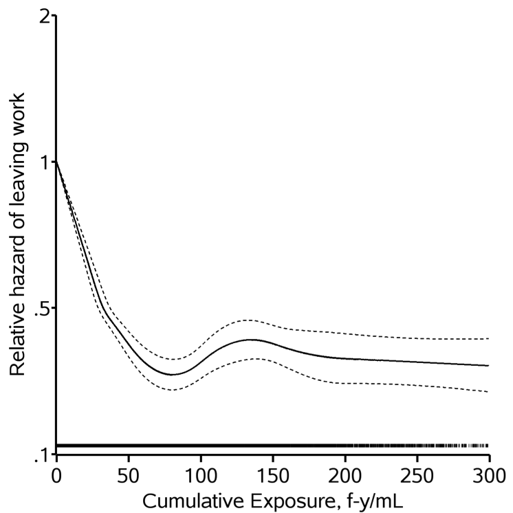
Relative to person-years exposed to below the median exposure value cumulated up to the prior year, the adjusted hazard ratio for leaving active employment (referent: actively employed, throughout) was 0.50 (95% CI, 0.46–0.55). This hazard ratio was not constant over age (P for heterogeneity < 0.001), whereby the hazard ratio became weaker with age (Fig. 2). For a continuous 100 fiber-year/mL increase in asbestos exposure cumulated up to the prior year, the adjusted hazard ratio for leaving active employment was 0.48 (95% CI, 0.42–0.54). Incorporating a 10-year exposure lag yielded a hazard ratio for leaving active employment of 0.71 (95% CI, 0.61–0.83) for a 100 fiber-year/mL increase in asbestos exposure cumulated up to the prior year. Finally, Figure A1 in the online Appendix shows the dose–response trend and 95% point-wise CIs for the relationship between asbestos exposure cumulated up to the prior year, and employment status. This figure demonstrates that the relative hazard of leaving work is below the null across the range of exposure values.

Component 2 is the association between employment status and subsequent exposure. Table 4 summarizes the number of person-years cross-classified by employment status and any asbestos exposure. Specifically, 88.3% of actively employed person-years (95% robust CI, 87.0–89.5) were classified as exposed to any asbestos. Lagging the indicator of any asbestos exposure (versus none) by 10 years yielded an unadjusted odds ratio for the association between employment status (referent = employed) and the lagged exposure (see Appendix 3) of 0.18 (95% robust CI, 0.17–0.20) based on the following person-years: exposed, left work, 9111; exposed, at work, 8093; unexposed, left work, 84,627; and unexposed, at work, 13,812. The adjusted odds ratio for the association between employment status and a 10-year lagged indicator of any asbestos exposure (Appendix 3; Model C2b) was 0.13 (95% robust CI, 0.12–0.15). Finally, using a linear regression model (Appendix 3, Model C2c), the adjusted mean difference in the log cumulative exposure between person-years not classified as actively employed (relative to person-years classified as actively employed) was −1.81 (95% robust CI, −1.89, −1.72).

Table 4.

Association between employment status and subsequent asbestos exposure for 2975 individuals followed during 115,643 person-years between 1940 and 2001

Employment status	Asbestos exposure		Total person-years	Exposure prevalence (%)*	95% CI†
	Any	None
At work	19,341	2564	21,905	88.3	87.0–89.5
Left work	0	93,738	93,738	0	–
Total person-years	19,341	96,302	115,643	16.7	15.9–17.6

CI = confidence interval.

^*Based on unlagged exposure values.

^†Confidence intervals estimated using robust variance.

Component 3 is the association between time-varying employment status and time to lung cancer mortality. Figure 3 depicts the complement of the crude Kaplan–Meier curves of lung cancer mortality stratified by time-varying employment status (logrank P < 0.0001).

Fig. 3.

Unadjusted Kaplan–Meier curves for the association between employment status and lung cancer mortality for 2975 individuals followed during 115,643 person-years between 1940 and 2001 with age as the time scale.

As can be seen in Figure 3, the cumulative proportion of lung cancer mortality was 5% by age 60 years while actively employed, and 5% by age 68 years after leaving active employment. Table 5 shows the number of lung cancer deaths, person-years at risk, and unadjusted and adjusted hazard ratios for the association between employment status and lung cancer mortality.

Table 5.

Association between employment status and lung cancer mortality for 2975 individuals followed during 115,643 person-years between 1940 and 2001

Employment status	Lung cancer deaths	Person- years	Unadjusted HR*	95% CI	Adjusted HR*,†	95% CI
At work	16	21,905	1		1
Left work	177	93,738	0.48	0.28–0.82	0.52	0.29–0.94
Total	193	115,643

CI = confidence interval; HR = hazard ratio.

^*Accounting for age as the time scale.

^†Adjusting for gender, race, and birth year (by restricted quadratic spline).

The adjusted hazard ratio was 0.52 (95% CI, 0.29–0.94) comparing time after leaving active employment to actively employed person-time. This hazard ratio was relatively constant over age (P for heterogeneity = 0.791. Restricting the analysis to person-years with no asbestos exposure in the prior year yielded a (less precise) hazard ratio of 0.42 (95% CI, 0.06–3.11). Further adjusting for subsequent exposure [to block W(j) → A(j) → T] resulted in a similar hazard ratio of 0.29 (95% CI, 0.04–2.16).

Discussion

Our findings indicate the presence of strong component associations of the healthy worker survivor bias in a cohort of textile factory workers from the southern United States. First, after accounting for age and other measured demographics, the hazard of leaving active employment among those exposed to greater than or equal to the median asbestos cumulated up to the prior year was half that among those exposed to less than the median. Second, we noted a large proportion of person-years classified as exposed to any asbestos while employed, but no person-years classified as exposed after termination of employment. Finally, after accounting for age and other measured demographics, the hazard of lung cancer mortality after termination of employment was about half that during years at work.

The association between prior asbestos exposure and employment status is the first component of the healthy worker survivor bias. The presence of this association precludes the use of employment status adjustment as a resolution for the confounding of exposure by employment status because of the bias induced by conditioning on a collider (Table 1) [5]. In this study, we found a strong inverse association between asbestos exposure cumulated up to the prior year and employment status. This strong inverse association existed across the range of exposure values (Fig. A1), and remained when we lagged the metric of cumulative exposure by 10 years.

The association between employment status and subsequent exposure is the source of nonpositivity in the healthy worker survivor bias [4]. We observed that 88% of individuals at work were classified as exposed to any asbestos, whereas none of the individuals were classified as exposed to any asbestos after having left work. This reflects a systematic or structural violation of the positivity assumption [8,35] because individuals cannot incur subsequent work-based exposure after having left work. Thus (in addition to the bias induced by conditioning on a collider), adjusting for a set of covariates that includes an indicator of employment status using standard methods would result in an “off-support” [9,36] estimate of the effect of occupational asbestos exposure on lung cancer mortality because of the model’s extrapolation of the association over regions where there are no data. Lagging the exposure variable may eliminate structural nonpositivity; however, standard analytic methods still require at least one of the three component associations to be rendered null. In these data, we observed a strong association between employment status and subsequent exposure, even after lagging the indicator of any exposure by 10 years, and when using a cumulative exposure metric.

The association between employment status and lung cancer mortality is the third component of the healthy worker survivor bias. Without this association, employment status will not confound the estimate of the effect of occupational asbestos exposure on time to lung cancer mortality. In this study, we found that the hazard of lung cancer mortality in those who left work was approximately half of that in those who remained on work (Table 3). This association was strongly confounded by age, but relatively constant over age. This inverse association between employment status and lung cancer mortality coincides with at least one previous study suggesting occupational mobility as a driver of the healthy worker survivor bias [37]. Individuals in more occupationally mobile categories would ostensibly be in a better position to find alternative employment earlier in life, as well as be more likely to avoid exposures (e.g., smoking) that increase the risk of death owing to lung cancer [38,39]. A positive association between occupational mobility and employment status, and an inverse association between occupational mobility and lung cancer mortality would induce an inverse association between employment status and lung cancer mortality [40], as found in the present study.

Two strategies commonly employed to minimize the healthy worker survivor bias are employment status adjustment [23] and exposure lagging [34]. The logic of causal diagrams can suggest whether use of such methods is justified by the data. For example, either before or after lagging, a lack of association between employment status and subsequent exposure or between employment status and mortality suggests no healthy worker survivor bias. If both of these associations are present, but there is no association between prior exposure and employment status, then adjusting for employment status should resolve the bias. When all three component associations are present, alternative methods are required (Table 1).

In this study, we found that lagging the exposure by 10 years did not eliminate the association between prior exposure and employment status, or between employment status and subsequent exposure. Researchers should be cautious, however, about using an exposure lag to minimize the healthy worker survivor bias. To avoid exposure misclassification, the lag used to account for the healthy worker survivor bias must coincide with the empirical induction period for the exposure [41].

The “presence” of a component association can be gauged by at least two criteria: Statistical significance and magnitude of association. The limitations of significance testing in observational research are well known [42,43]. Furthermore, prior simulation research has suggested that the performance of standard methods is inversely related to the magnitude of the component associations [4]. As such, although both statistical significance and magnitude of association are likely to be important, we believe the latter criterion to be of more relevance in an occupational setting with no random assignment mechanism. In our study, all three component associations were both statistically significant and relatively strong in magnitude. Moreover, this was true whether we assessed the component associations using extended Kaplan–Meier curves, or using continuous or binary exposure variables with a number of different regression models. Finally, it would be tempting to predict the overall direction of the healthy worker survivor bias using the estimated magnitudes of each component association, and the method of signed directed acyclic graphs [40,44]. However, this method is not justified in the presence of a collider, such as our indicator of employment status [40].

As is common in occupational epidemiology, we were lacking information on individual smoking history and intermittent time off work, and used a regression model to estimate exposure values from a job/task exposure matrix. Following standard practice, we assume independent censoring conditional on measured covariates for all survival analyses. Furthermore, our aim was to present a simple heuristic to suggest whether standard methods are justified when the healthy worker survivor bias is suspected. We did not assess whether the observed component associations were modified by relevant characteristics. Given the complex social context in which exposure, employment status, and mortality are related [45], a nuanced substantive analysis of each component association is warranted. Finally, although our analysis was restricted to mortality as an outcome, we note that the proposed method could be applied to other outcomes as well when the healthy worker survivor bias is suspected.

Using causal diagrams, we isolated the component associations that are collectively responsible for the time-varying confounding and nonpositivity underlying the healthy worker survivor bias. Despite limitations, the example demonstrated that these three component associations were present. Indeed, our exploration of these component relations is strengthened by the use of a large cohort with well-characterized mortality and only 9% loss to follow-up over a 60-year period. Our findings imply that, for these data, commonly used methods such as exposure lagging or employment status adjustment will not reduce the healthy worker survivor bias. In future research, we intend to assess the association between asbestos exposure and lung cancer mortality using methods that can account for time-varying confounding, including g-estimation of a structural nested model [13] and the parametric g-formula [10].

Appendix 1. Mortality ascertainment

Vital status through 1978 was determined using information from the Social Security Administration, Internal Revenue Service, the U.S. Postal Mail Correction Service, state driver’s license files, and state vital statistics offices [19,20]. Between 1979 and 2001, the U.S. NDI was used to obtain vital status. Workers that were confirmed alive on January 1, 1979, and not shown to be deceased by the NDI between 1979 and 2001 were considered to be alive as of 2001. Workers lost to follow-up before January 1, 1979, were censored at the date they were last known to be alive. Before 1979, death certificates were obtained from the state vital records offices and the underlying cause of death was coded by a qualified nosologist. After 1979, the NDI provided underlying causes of death. All deaths were coded according to the revision of the International Classification of Diseases (ICD) in effect at the time of death. Lung cancer mortality was defined as ICD-8 and ICD-9 codes 162–163, and ICD-10 codes C33-C34.

Appendix 2. Exposure assessment

Ambient asbestos concentrations were estimated using 5952 sampling measurements taken between 1930 and 1975 analyzed using phase contrast microscopy [18]. To create a job/task exposure matrix, the factory was divided into 16 exposure zones corresponding to physically well-defined areas. Jobs within each exposure zone were assigned to one of four uniform job categories based on the tasks associated with that job. Job/task-specific average asbestos concentrations in the ambient air surrounding 16 exposure zones were estimated using a department, task, and calendar time-specific exposure matrix [18]. These estimates were linked to individuals using detailed job histories based on personnel records collected by the company beginning in 1930, compiled and microfilmed by the U.S. Public Health Service in 1968, and updated, digitized, and quality controlled in 1978 [15]. Each day during the years in which the person was not employed was assigned a zero asbestos exposure.

During the years in which the person was employed, each day was assigned a department, task, and calendar period specific average asbestos exposure in units of chrysotile fibers longer than 5 µm/mLair. Following previous research [16–21], annual exposure levels, in fiber-years per milliliter, were calculated as the product of duration of exposure in that calendar year and the department, task, and calendar period specific average concentration of chrysotile fibers longer than 5 µm/mL air to which an individual was exposed.

Appendix 3. Statistical methods

To assess the component associations of the healthy worker survivor bias, we arranged our data into person-year format with i = 1 to 2975 subjects, each with m_i∈[1, 62] observations representing a year on study at age j (the range for j was 13–101 years), for a total of 115,643 observations. Component 1 is the association between prior asbestos exposure and employment status. Because no individuals who left active employment returned to work, we modeled this association with Cox proportional hazards regression [28] using the counting process format [46,47] to account for time-varying prior exposures by defining the hazard of leaving active employment for individual i at age j as

$${\lambda }_{\mathrm{i}}(\mathrm{j})={\lambda }_0(\mathrm{j})\text{exp}\{{\beta }_{1}I[A_{\mathrm{i}}(\mathrm{j}-1)\ge 5.4]+{\beta }_{2}I({\text{non - Caucasian}}_{\mathrm{i}})+{\beta }_{3}I({\text{female}}_{\mathrm{i}})+g({\text{birth year}}_{\mathrm{i}})\mathbf{\beta }\}$$ Model C1a

where λ₀(j) is the baseline hazard function, and where parameters in exp{·} were estimated by maximizing the partial likelihood [48]. Here, and throughout, I(·) represents the indicator function that takes a value of one when the argument (·) is true (zero otherwise), g(·) returns a 1 × 4 vector containing restricted quadratic spline basis functions for argument (·) with knots as defined in the text, and β represents a 4 × 1 vector of parameters for each basis function. Furthermore, $A_{\mathrm{i}}(\mathrm{j})=\sum _{\mathrm{k}\ge \mathrm{j}}{X}_{\mathrm{i}}(\mathrm{k})$ is a measure of cumulative exposure in fiber-years per milliliter for individual i accrued up to age j. To assess the association between time to leaving work and a 100 fiber-year/mL increase in cumulative asbestos exposure, we replaced I[A_i(j − 1) ≥ 5.4] in model C1a with a continuous measure of cumulative asbestos exposure accrued up to the prior year, A_i(j − 1).

Exposure lagging has been suggested as potential method to control the healthy worker survivor bias [34]. Following standard practice [[49], p. 170], we explored the association for Component 1 using a 10-year lag by replacing A_i(j) with A_i(j − 10). If individual i was not in the study at age j−10, the continuous exposure value used to calculate A_i(j) was set to zero. Finally, to assess dose response trends between cumulative exposure and the hazard of leaving work, we used a Cox proportional hazards model defined as

$${\lambda }_{\mathrm{i}}(\mathrm{j})={\lambda }_0(\mathrm{j})\text{exp}\{g[A_{\mathrm{i}}(\mathrm{j})]\mathbf{\beta }\},$$ Model C1b

where λ₀(j) is the baseline hazard function, and where parameters in exp(·) were estimated by maximizing the partial likelihood. This model was used to plot the relative hazard over all j across values of A(j) (Fig. A1).

Component 2 is the association between having left active employment and an indicator of any asbestos exposure. Because individuals who left active employment can no longer be classified as exposed, this component is the source of nonpositivity. To avoid estimation problems owing to quasi-complete separation of data points [50,51] resulting from nonpositivity, we estimated the proportion of person-years exposed while at work using an intercept only logistic regression model defined as

$$P\{I[X_{\mathrm{i}}(\mathrm{j})>0]\}=W_{\mathrm{i}}(\mathrm{j})\times {[1+\text{exp}(-{\beta }_0)]}^{-1}$$ Model C2a

where β₀ was estimated using generalized estimating equations [32] with an independent working covariance matrix [33]. Lagging the exposure variable by 10 years resulted in a non-zero proportion of exposed person-years within both strata of employment status, allowing us to estimate adjusted odds ratios with a logistic regression model defined as

$$P\{I[X_{\mathrm{i}}(\mathrm{j}-10)>0]\}={\{1+\text{exp}[-({\beta }_0+{\beta }_1{W}_{\mathrm{i}}(\mathrm{j})+{\beta }_{2}I({\text{female}}_{\mathrm{i}})+{\beta }_{3}I({\text{non - Caucasian}}_{\mathrm{i}})+g({\text{birth year}}_{\mathrm{i}}){\mathbf{\beta }}_{\text{birth year}}+g({\text{age}}_{\mathrm{i}}){\beta }_{\text{age}})]\}}^{-1}$$ Model C2b

with parameters for this model estimated using generalized estimating equations with an independent working covariance matrix. Finally, we assessed the adjusted association between a continuous metric for cumulative exposure and employment status by defining a linear regression model as

$$\text{log}[A_{\mathrm{i}}(\mathrm{j})]={\beta }_0+{\beta }_1{W}_{\mathrm{i}}(\mathrm{j})+{\beta }_{2}I({\text{non - Caucasion}}_{\mathrm{i}})+{\beta }_{3}I({\text{female}}_{\mathrm{i}})+g({\text{birth year}}_{\mathrm{i}}){\beta }_{\text{birth year}}+g({\text{age}}_{\mathrm{i}}){\beta }_{\text{age}}+{\epsilon }_{\text{ij}}$$ Model C2c

where ε_ij~N(0, σ²) and with parameters estimated using generalized estimating equations with an independent working covariance matrix.

Component 3 is the association between leaving active employment and lung cancer mortality. We modeled this association using Cox proportional hazards regression by defining the hazard of lung cancer mortality at age j as

$${\gamma }_{\mathrm{i}}(\mathrm{j})={\gamma }_0(\mathrm{j})\text{exp}\{{\beta }_1{W}_{\mathrm{i}}(\mathrm{j})+{\beta }_{2}I({\text{non - Caucasion}}_{\mathrm{i}})+{\beta }_{3}I({\text{female}}_{\mathrm{i}})+g({\text{birth year}}_{\mathrm{i}})\mathbf{\beta }\}$$ Model C3

where γ₀(j) is the baseline hazard function, and where parameters in exp{·} were estimated by maximizing the partial likelihood.

References

- 1.Arrighi HM, Hertz-Picciotto I. The evolving concept of the healthy worker survivor effect. Epidemiology. 1994;5(2):189–186. doi: 10.1097/00001648-199403000-00009. [DOI] [PubMed] [Google Scholar]
- 2.Pearl J. Causal diagrams for empirical research. Biometrika. 1995;82(4):669–688. [Google Scholar]
- 3.Hernán MA, Hernández-Diaz S, Robins JM. A structural approach to selection bias. Epidemiology. 2004;15(5):615–625. doi: 10.1097/01.ede.0000135174.63482.43. [DOI] [PubMed] [Google Scholar]
- 4.Naimi AI, Cole SR, Westreich D, Richardson D. A comparison of methods to estimate the hazard ratio under conditions of time-varying confounding with nonpositivity. Epidemiology. 2011;22(5):718–723. doi: 10.1097/EDE.0b013e31822549e8. [DOI] [PMC free article] [PubMed] [Google Scholar]
- 5.Cole SR, Piatt RW, Schisterman EF, Chu H, Westreich D, Richardson D, et al. Illustrating bias due to conditioning on a collider. Intl J Epidemiol. 2010;39(2):417–420. doi: 10.1093/ije/dyp334. [DOI] [PMC free article] [PubMed] [Google Scholar]
- 6.Hernán MA, Robins JM. Estimating causal effects from epidemiological data. J Epidemiol Community Health. 2006;60(7):578–586. doi: 10.1136/jech.2004.029496. [DOI] [PMC free article] [PubMed] [Google Scholar]
- 7.Cole SR, Hernán MA. Constructing inverse probability weights for marginal structural models. Am J Epidemiol. 2008;168(6):656–664. doi: 10.1093/aje/kwn164. [DOI] [PMC free article] [PubMed] [Google Scholar]
- 8.Westreich D, Cole SR. Invited commentary: positivity in practice. Am J Epidemiol. 2010;171(6):674–677. doi: 10.1093/aje/kwp436. [DOI] [PMC free article] [PubMed] [Google Scholar]
- 9.Manski CF. Identification problems in the social sciences. Cambridge, MA: Harvard University Press; 1995. [Google Scholar]
- 10.Robins JM. A new approach to causal inference in mortality studies with a sustained exposure period–application to control of the healthy worker survivor effect. Mathematical Modelling. 1986;7:1393–1512. [Google Scholar]
- 11.Taubman SL, Robins JM, Mittleman MA, Hernán MA. Intervening on risk factors for coronary heart disease: an application of the parametric g-formula. Int J Epidemiol. 2009;38(6):1599–1611. doi: 10.1093/ije/dyp192. [DOI] [PMC free article] [PubMed] [Google Scholar]
- 12.Robins J, Hernán M. Estimation of the causal effects of time-varying exposures. In: Fitzmaurice G, Davidian M, Verbeke G, Molenberghs G, editors. Advances in longitudinal data analysis. Boca Raton, FL: Chapman & Hall; 2009. pp. 553–599. [Google Scholar]
- 13.Robins J. The analysis of randomized and non-randomized AIDS treatment trials using a new approach to causal inference in longitudinal studies. In: Sechrest L, Freeman HAM, editors. Health Service research methodology: a focus on AIDS. Washington, D.C: U.S. Public Health Service, National Center for Health Services Research; 1989. pp. 113–159. [Google Scholar]
- 14.Robins JM. Structural nested failure time models. In: Andersen P, Keiding N, editors. The encyclopedia of biostatistics. Chichester, UK: John Wiley and Sons; 1998. [Google Scholar]
- 15.Dement J. Estimation of dose and evaluation of dose-response in a retrospective cohort mortality study of chrysotile asbestos textile workers. Doctoral Dissertation. University of North Carolina at Chapel Hill. 1980 [Google Scholar]
- 16.Dement JM, Brown DP. Lung cancer mortality among asbestos textile workers: a review and update. Ann Occup Hyg. 1994;38(4):525–532. doi: 10.1093/annhyg/38.4.525. [DOI] [PubMed] [Google Scholar]
- 17.Dement JM, Brown DP, Okun A. Follow-up study of chrysotile asbestos textile workers: cohort mortality and case-control analyses. Am J Ind Med. 1994;26(4):431–447. doi: 10.1002/ajim.4700260402. [DOI] [PubMed] [Google Scholar]
- 18.Dement JM, Harris RL, Symons MJ, Shy CM. Exposures mortality among chrysotile asbestos workers Part I: exposure estimates. Am J Industrial Med. 1983;4(3):399–419. doi: 10.1002/ajim.4700040303. [DOI] [PubMed] [Google Scholar]
- 19.Dement JM, Harris RL, Symons MJ, Shy CM. Exposures mortality among chrysotile asbestos workers Part II: mortality. Am J Industrial Med. 1983;4(3):421–433. doi: 10.1002/ajim.4700040304. [DOI] [PubMed] [Google Scholar]
- 20.Hein MJ, Stayner LT, Lehman E, Dement JM. Follow-up study of chrysotile textile workers: cohort mortality and exposure-response. Occup Environ Med. 2007;64(9):616–625. doi: 10.1136/oem.2006.031005. [DOI] [PMC free article] [PubMed] [Google Scholar]
- 21.Stayner L, Smith R, Bailer J, Gilbert S, Steenland K, Dement J, et al. Exposure-response analysis of risk of respiratory disease associated with occupational exposure to chrysotile asbestos. Occup Environ Med. 1997;54(9):646–652. doi: 10.1136/oem.54.9.646. [DOI] [PMC free article] [PubMed] [Google Scholar]
- 22.Glymour MM, Greenland S. Causal diagrams. In: Rothman KJ, Greenland S, Lash TL, editors. Modern epidemiology. New York: Wolters Kluwer | Lippin-cott Williams & Wilkins; 2008. pp. 183–209. [Google Scholar]
- 23.Gilbert ES, Marks S. An analysis of the mortality of workers in a nuclear facility. Radiation Res. 1979;79(1):122–148. [PubMed] [Google Scholar]
- 24.Eisen E, Robins J. Healthy worker effect. In: El-Shaarawi A, Piegorsch W, editors. Encyclopedia of environmetrics. New York: John-Wiley & Sons; 2002. [Google Scholar]
- 25.Snapinn SM, Jiang Q, Iglewicz B. Illustrating the impact of a time-varying covariate with an extended Kaplan-Meier estimator. Am Stat. 2005;59(4):301–337. [Google Scholar]
- 26.Lamarca R, Alonso J, Gómez G, Muñoz Á. Left-truncated data with age as time scale: an alternative for survival analysis in the elderly population. J Gerontol A Biol Sci Med Sci. 1998;53A(5):M337–M343. doi: 10.1093/gerona/53a.5.m337. [DOI] [PubMed] [Google Scholar]
- 27.Klein JP, Moeschberger ML. Statistics for biology and health. New York: Springer-Verlag; 2003. Survival analysis: techniques for censored and truncated data; pp. 1431–8776. [Google Scholar]
- 28.Cox DR. Regression models and life-tables. J R Stat Soc B Meth. 1972;34(2):187–220. [Google Scholar]
- 29.Efron B. The efficiency of Cox’s likelihood function for censored data. J Am Stat Assoc. 1977;72(359):557–565. [Google Scholar]
- 30.Kom EL, Graubard BI, Midthune D. Time-to-event analysis of longitudinal follow-up of a survey: choice of the time-scale. Am J Epidemiol. 1997;145(1):72–80. doi: 10.1093/oxfordjournals.aje.a009034. [DOI] [PubMed] [Google Scholar]
- 31.Howe C, Cole S, Westreich D, Greenland S, Napravnik S, Eron J. Splines for trend analysis and continuous confounder control. Epidemiology. 2011;22(6):874–875. doi: 10.1097/EDE.0b013e31823029dd. [DOI] [PMC free article] [PubMed] [Google Scholar]
- 32.Liang K-Y. Zeger SL Longitudinal data analysis using generalized linear models. Biometrika. 1986;73(1):13–22. [Google Scholar]
- 33.Pepe MS, Anderson GL. A cautionary note on inference for marginal regression models with longitudinal data and general correlated response data. Commun Stat Simul Comput. 1994;23(4):939–951. [Google Scholar]
- 34.Gilbert ES. Some confounding factors in the study of mortality and occupational exposures. Am J Epidemiol. 1982;116(1):177–188. doi: 10.1093/oxfordjournals.aje.a113392. [DOI] [PubMed] [Google Scholar]
- 35.Petersen ML, Porter KE, Gruber S, Wang Y, van der Laan MJ. Diagnosing and responding to violations in the positivity assumption. Stat Methods Med Res. 2010:1–24. doi: 10.1177/0962280210386207. [DOI] [PMC free article] [PubMed] [Google Scholar]
- 36.Messer LC, Oakes JM, Mason S. Effects of socioeconomic and racial residential segregation on preterm birth: a cautionary tale of structural confounding. Am J Epidemiol. 2010;171(6):664–673. doi: 10.1093/aje/kwp435. [DOI] [PubMed] [Google Scholar]
- 37.Siebert U, Rothenbacher D, Daniel U, Brenner H. Demonstration of the healthy worker survivor effect in a cohort of workers in the construction industry. Occup Environ Med. 2001;58(12):774–779. doi: 10.1136/oem.58.12.774. [DOI] [PMC free article] [PubMed] [Google Scholar]
- 38.Melchior M, Goldberg M, Krieger N, Kawachi I, Menvielle G, Zins M, et al. Occupational class, occupational mobility and cancer incidence among middle-aged men and women: a prospective study of the French GAZEL cohort*. Cancer Causes Control. 2005;16(5):515–524. doi: 10.1007/s10552-004-7116-0. [DOI] [PubMed] [Google Scholar]
- 39.Marshall B, Chevalier A, Garillon C, Goldberg M, Coing F. Socioeconomic status, social mobility and cancer occurrence during working life: a case-control study among French electricity and gas workers. Cancer Causes Control. 1999;10(6):495–502. doi: 10.1023/a:1008921720493. [DOI] [PubMed] [Google Scholar]
- 40.VanderWeele TJ, Hernan MA, Robins JM. Causal directed acyclic graphs and the direction of unmeasured confounding bias. Epidemiology. 2008;19(5):720–708. doi: 10.1097/EDE.0b013e3181810e29. [DOI] [PMC free article] [PubMed] [Google Scholar]
- 41.Rothman KJ. Induction and latent periods. Am J Epidemiol. 1981;114(2):253–259. doi: 10.1093/oxfordjournals.aje.a113189. [DOI] [PubMed] [Google Scholar]
- 42.Stang A, Poole C, Kuss O. The ongoing tyranny of statistical significance testing in biomedical research. Eur J Epidemiol. 2010;25(4):225–230. doi: 10.1007/s10654-010-9440-x. [DOI] [PubMed] [Google Scholar]
- 43.Greenland S. Randomization, statistics, and causal inference. Epidemiology. 1990;l(6):421–429. doi: 10.1097/00001648-199011000-00003. [DOI] [PubMed] [Google Scholar]
- 44.VanderWeele TJ, Robins JM. Signed directed acyclic graphs for causal inference. J R Stat Soc B. 2010;72(1):111–127. doi: 10.1111/j.1467-9868.2009.00728.x. [DOI] [PMC free article] [PubMed] [Google Scholar]
- 45.Wilcosky T, Wing S. The healthy worker effect: selection of workers and work forces. Scand J Work. Environ Health. 1987;13(1):70–72. doi: 10.5271/sjweh.2078. [DOI] [PubMed] [Google Scholar]
- 46.Andersen PK, Gill RD. Cox’s Regression model for counting processes: a large sample study. Ann Stat. 1982;10(4):1100–1120. [Google Scholar]
- 47.Therneau TM. Statistics for biology and health. New York: Springer; 2000. Modeling survival data: extending the Cox model. [Google Scholar]
- 48.Cox DR. Partial likelihood. Biometrika. 1975;62(2):269–276. [Google Scholar]
- 49.Checkoway H. Monographs in epidemiology and biostatistics. vol. 34. Oxford, New York: Oxford University Press; 2004. Research methods in occupational epidemiology. [Google Scholar]
- 50.Albert A, Anderson JA. On the existence of maximum likelihood estimates in logistic regression models. Biometrika. 1984;71(1):1–10. [Google Scholar]
- 51.Allison P, Altman M, Gill J, McDonald MP. Numerical issues in statistical computing for the social scientist. John Wiley & Sons; 2004. Convergence problems in logistic regression; pp. 238–252. [Google Scholar]
Associated Data
This section collects any data citations, data availability statements, or supplementary materials included in this article.