A Convex Formulation for Learning a Shared Predictive Structure from Multiple Tasks

Abstract

In this paper, we consider the problem of learning from multiple related tasks for improved generalization performance by extracting their shared structures. The alternating structure optimization (ASO) algorithm, which couples all tasks using a shared feature representation, has been successfully applied in various multitask learning problems. However, ASO is nonconvex and the alternating algorithm only finds a local solution. We first present an improved ASO formulation (iASO) for multitask learning based on a new regularizer. We then convert iASO, a nonconvex formulation, into a relaxed convex one (rASO). Interestingly, our theoretical analysis reveals that rASO finds a globally optimal solution to its nonconvex counterpart iASO under certain conditions. rASO can be equivalently reformulated as a semidefinite program (SDP), which is, however, not scalable to large datasets. We propose to employ the block coordinate descent (BCD) method and the accelerated projected gradient (APG) algorithm separately to find the globally optimal solution to rASO; we also develop efficient algorithms for solving the key subproblems involved in BCD and APG. The experiments on the Yahoo webpages datasets and the Drosophila gene expression pattern images datasets demonstrate the effectiveness and efficiency of the proposed algorithms and confirm our theoretical analysis.

1 Introduction

In many real-world pattern classification problems [1], [2], each of the tasks can often be divided into several subtasks which are inherently related. The subtasks can be solved traditionally via the single-task learning (STL) scheme, in which the subtasks are learned independently, i.e., one task is learned at a time. Over the past decade, there has been an upsurge of interest in multitask learning (MTL) [3], [4], [5], [6], [7], [8], [9]. MTL aims to improve the generalization performance of the classifiers by learning from multiple related subtasks. This can be achieved by learning the tasks simultaneously and meanwhile exploiting the intrinsic relatedness among the tasks. Based on the MTL scheme, some useful information can be shared across the tasks, thus facilitating individual task learning. It is particularly desirable to share such knowledge across the tasks when there are a number of related tasks but only limited training data is available for each one. MTL has been applied successfully in several application domains such as bioinformatics [10], medical image analysis [11], web search ranking [12], and computer vision [13], [14].

The problem of multitask learning has been addressed by many researchers. Thrun and O’Sullivan [15] proposed a task-clustering (TC) algorithm to cluster multiple learning tasks into groups of mutually related tasks (by measuring the generalization performance resulting from sharing the same distance metric among the task pairs). Caruana [3] studied multitask learning using the backpropagation net and demonstrated the effectiveness of MTL in several real-world applications. Baxter [16] introduced an inductive bias learning model to determine a common optimal hypothesis space for similar tasks. Bakker and Heskes [17] employed a Bayesian approach for multitask learning in which the model parameters are shared explicitly or are loosely connected through a joint prior distribution that can be determined from the data. Lawrence and Platt [18] applied the multitask informative vector machine to infer the parameters for a Gaussian process. Based on a hierarchical Bayesian framework, Schwaighofer et al. [19] subsequently proposed learning nonparametric covariance matrices from multitask data via EM-algorithm, which was further improved by Yu et al. in [20]. Zhang et al. [21] proposed to model the task relatedness via the latent independent components, which is a hierarchical Bayesian model based on the traditional ICA. Jacob et al. [22] proposed to learn multiple tasks by assuming that tasks can be clustered into different groups and the task weight vectors within a group are similar to each other. In [23], [24], the kernel functions with a task-coupling parameter are employed for modeling the relationship among multiple related tasks.

Recently, there has been growing interest in studying multitask learning in the context of feature learning (selection). Jebara [25] considered the problem of feature selection with SVM across the tasks. Obozinski et al. [26] presented multitask joint covariate selection based on a generalization of 1-norm regularization. Argyriou et al. [27] proposed to learn a common sparse representation from multiple tasks, which can be solved via an alternating optimization algorithm. One following work in [8] proposed the convex multitask feature learning formulation and showed that the alternating optimization algorithm converges to a global optimum of the proposed formulation. Note that the MTL formulation in [8] is essentially equivalent to the approach of employing the trace norm as a regularization for multitask learning [28], [29], [30]. Ando and Zhang [5] proposed the alternating structure optimization (ASO) to learn shared predictive structures from multiple related tasks. In ASO, a separate linear classifier is trained for each task and dimension reduction is applied on the classifier space, computing low-dimensional structures with the highest predictive power. However, this framework is nonconvex and the alternating structure optimization procedure is not guaranteed to find a global optimum, as pointed out in [5], [8]. The relationship between ASO and clustered MTL was studied in [31].

In this paper, we consider the problem of learning a shared structure from multiple related tasks following the approach in [5]. We present an improved ASO formulation (called iASO) using a new regularizer. The improved formulation is nonconvex; we show that it can be converted into a relaxed convex formulation (called rASO). In addition, we present a theoretical condition under which rASO finds a globally optimal solution to its nonconvex counterpart iASO. rASO can be equivalently reformulated as a semidefinite program (SDP), which is, however, not scalable to large datasets.

We proposed to employ the block coordinate descent (BCD) method [32] to solve rASO. In BCD, the optimization variables are optimized via two alternating computation procedures; we develop efficient algorithms for the procedures in BCD and show that the BCD algorithm converges to a global optimum of rASO. We also propose to employ the accelerated projected gradient (APG) algorithm to solve rASO. APG belongs to the category of the first-order methods and its global convergence rate is optimal among all the first-order methods [33], [34]. We show that the subproblem in each iteration of APG can be solved efficiently. We also further discuss the computation cost in the BCD method and the APG algorithm for solving rASO, respectively. We have conducted experiments on the Yahoo webpages datasets [35] and the Drosophila gene expression pattern images datasets [36]. The experimental results demonstrate the effectiveness of the proposed MTL formulation and the efficiency of the proposed optimization algorithms. Results also confirm our theoretical analysis, i.e., rASO finds a globally optimal solution to its nonconvex counterpart iASO under certain conditions.

The remainder of this paper is organized as follows: In Section 2, we present the improved MTL formulation iASO; in Section 3, we show how to convert the nonconvex iASO into the convex relaxation rASO; in Sections 4 and 5, we detail the BCD algorithm and the APG algorithm, respectively, for solving rASO; in Section 6, we present a theoretical condition under which a globally optimal solution to iASO can be obtained via rASO; we report the experimental results in Section 7; and the paper concludes in Section 8.

Notations

Denote ${\mathbb{N}}_n=\{1,\dots ,n\}$. Denote $A\underset{¯}{\prec }B$ if and only if B – A is positive semidefinite (PSD). Let tr(_X) be the trace. 0 and I denote the zero matrix and the identity matrix of appropriate sizes, respectively.

2 Multitask Learning Framework

Assume that we are given _m supervised (binary-class) learning tasks. Each of the learning tasks is associated with a predictor f_l and training data $\left\{\right(x_1^{\ell },y_1^{\ell }),\dots ,(x_{n_{\ell }}^{\ell },y_{n_{\ell }}^{\ell }\left)\right\}\subset {\mathbb{R}}^d\times \{-1,1\}(\ell \in {\mathbb{N}}_m)$. We focus on linear predictors $f_{\ell }\left(x\right)=u_{\ell }^{T}x$ where u_l is the weight vector for the lth task.

The alternating structure optimization algorithm learns predictive functional structures from multiple related tasks. Specifically, it learns all m predictors {f1; … ; f_m} simultaneously by exploiting a shared feature space in a simple linear form of low-dimensional feature map Θ across the m tasks. Formally, the predictor f_l can be expressed as

$$f_{\ell }\left(x\right)=u_{\ell }^{T}x=w_{\ell }^{T}x+v_{\ell }^T\Theta x,$$ (1)

where the structure parameter Θ takes the form of an h × d matrix with orthonormal rows as

$$\Theta {\Theta }^T=\mathrm{I},$$

and u_l, w_l, and v_l are the weight vectors for the full feature space, the high-dimensional feature space, and the shared low-dimensional feature space, respectively. Note that since h specifies the shared low-dimensional feature space of the m tasks, without loss of generality h can always be chosen to be smaller than m and d. Mathematically, ASO can be formulated as the following optimization problem:

$$\begin{array}{cc}\hfill \underset{\{u_{\ell },v_{\ell }\},\Theta }{\min }& \sum _{\ell =1}^m\left(\frac{1}{n_{\ell }}\sum _{i=1}^{n_{\ell }}L(u_{\ell }^T{x}_i^{\ell },y_i^{\ell })+a\alpha {\Vert w_{\ell }\Vert }^2\right)\hfill \\ \hfill \text{subject to}& \Theta {\Theta }^T=\mathrm{I},\hfill \end{array}$$ (2)

where L(·) is a convex loss function, ∥w_l∥² is the regularization term (w_l = u_l − Θ^T_vl) controlling the relatedness among m tasks, and α is prespecified nonnegative parameter.

The optimization problem in (2) is nonconvex due to its orthonormal constraint and the regularization term in terms of u_l, v_l, and Θ. We present an improved ASO formulation (called iASO) given by

$$\begin{array}{cc}\hfill \left({\mathrm{F}}_0\right)\underset{\{u_{\ell },v_{\ell }\},\Theta }{\min }& \sum _{\ell =1}^m\left(\frac{1}{n_{\ell }}\sum _{i=1}^{n_{\ell }}L(u_{\ell }^T{x}_i^{\ell },y_i^{\ell })+g_{\ell }(u_{\ell },v_{\ell },\Theta )\right),\hfill \\ \hfill \text{subject to}& \Theta {\Theta }^T=\mathrm{I},\hfill \end{array}$$ (3)

where g_l(u_l; v_l, Θ) is defined as

$$g_{\ell }(u_{\ell },v_{\ell },\Theta )=\alpha {\Vert u_{\ell }-{\Theta }^T{v}_{\ell }\Vert }^2+\beta {\Vert u_{\ell }\Vert }^2.$$ (4)

The regularization function in (4) controls the task relatedness (via the first component) as well as the complexity of the predictor functions (via the second component) as commonly used in traditional regularized risk minimization formulations for supervised learning. Note that α and β are prespecified coefficients, indicating the importance of the corresponding regularization components, respectively. For simplicity, we use the same α and β for all tasks. The discussion below can be easily extended to the case where α and β are different for different tasks.

The iASO formulation (F₀) in (3) subsumes several multitask learning algorithms as special cases: It reduces to the ASO algorithm in (2) by setting β = 0 in (4), and it reduces to m independent quadratic programs (QP) by setting α = 0. It is worth noting that iASO is nonconvex. In the next section, we convert iASO into a (relaxed) convex formulation, which admits a globally optimal solution.

3 A Convex Multitask Learning Formulation

In this section, we consider a convex relaxation of the nonconvex F₀ (iASO).

The optimal ${\left\{v_{\ell }^{\ast }\right\}}_{\ell =1}^m$ to (3) can be expressed in the form of a function on Θ and ${\left\{u_{\ell }\right\}}_{\ell =1}^m$. It can be verified that $v_{\ell }^{\ast }=\Theta u_{\ell }=\arg {\min }_{v_{\ell }}{g}_{\ell }(u_{\ell },v_{\ell },\Theta ),\ell \in {\mathbb{N}}_m$. Let $U=[u_1,\dots ,u_m]\in {\mathbb{R}}^{d\times m}$ and $V=[v_1,\dots ,v_m]\in {\mathbb{R}}^{h\times m}$. The optimal V* to (3) is given by V* = ΘU. Therefore, we denote

$$\begin{array}{cc}\hfill G_0(U,\Theta )& =\underset{V}{\min }\sum _{\ell =1}^m{g}_{\ell }(u_{\ell },v_{\ell },\Theta )\hfill \\ \hfill & =\alpha \mathrm{tr}\left(U^T\right((1+\eta )\mathrm{I}-{\Theta }^T\Theta \left)U\right),\hfill \end{array}$$ (5)

where η = β/α > 0. Moreover, it can be verified that (1 + η)I − Θ^TΘ = η(1 + η)(ηI + Θ^TΘ)⁻¹. We can reformulate G₀(U, Θ) into an equivalent form as

$$G_1(U,\Theta )=\alpha \eta (1+\eta )\mathrm{tr}\left(U^T{(\eta \mathrm{I}+{\Theta }^T\Theta )}^{-1}U\right).$$ (6)

Since the loss term in (3) is independent of the optimization variables ${\left\{v_{\ell }\right\}}_{\ell =1}^m$, F₀ can be equivalently transformed into the following optimization problem F₁ with optimization variables Θ and U:

$$\begin{array}{cc}\hfill \left({\mathrm{F}}_1\right)\underset{\left\{u_{\ell }\right\},\Theta }{\min }& \sum _{\ell =1}^m\left(\frac{1}{n_{\ell }}\sum _{i=1}^{n_{\ell }}L(u_{\ell }^T{x}_i^{\ell },y_i^{\ell })\right)+G_1(U,\Theta )\hfill \\ \hfill \text{subject to}& \Theta {\Theta }^T=\mathrm{I},\hfill \end{array}$$ (7)

where G₁(U, Θ) is defined in (6).

3.1 Convex Relaxation

The orthonormality constraint in (7) is nonconvex; so is the optimization problem F₁. We propose to convert F₁ into a convex formulation by relaxing its feasible domain into a convex set. Let ${\mathcal{M}}_e=\{M_e\mid M_e={\Theta }^T\Theta ,\Theta {\Theta }^T=\mathrm{I},\Theta \in {\mathbb{R}}^{h\times d}\}$. It has been known [37] that the convex hull [38] of ${\mathcal{M}}_e$ can be precisely expressed as the convex set

$${\mathcal{M}}_c=\{M_c\mid \mathrm{tr}(M_c)=h,0,\underset{¯}{\prec }{M}_c\underset{¯}{\prec }\mathrm{I}\},$$

and each element in ${\mathcal{M}}_e$ is referred to as an extreme point of ${\mathcal{M}}_e$. Since ${\mathcal{M}}_c$ consists of all convex combinations of the elements in ${\mathcal{M}}_e$, ${\mathcal{M}}_c$ is the smallest convex set that contains ${\mathcal{M}}_e$.

To convert the nonconvex problem F₁ into a convex formulation, we replace Θ^TΘ with M in (7), and naturally relax its feasible domain into a convex set based on the relationship between ${\mathcal{M}}_e$ and ${\mathcal{M}}_c$ presented above; this results in an optimization problem F₂ (called rASO) as

$$\begin{array}{cc}\hfill \left({\mathrm{F}}_2\right)\underset{\left\{u_{\ell }\right\},M}{\min }& \sum _{\ell =1}^m\left(\frac{1}{n_{\ell }}\sum _{i=1}^{n_{\ell }}L(u_{\ell }^T{x}_i^{\ell },y_i^{\ell })\right)+G_2(U,M)\hfill \\ \hfill \text{subject to}& \mathrm{tr}\left(M\right)=h,0\underset{¯}{\prec }M\underset{¯}{\prec }\mathrm{I},\hfill \end{array}$$ (8)

where G₂(U, M) is defined as

$$G_2(U,M)=\alpha \eta (1+\eta )\mathrm{tr}\left(U^T{(\eta \mathrm{I}+M)}^{-1}U\right).$$ (9)

It follows from [39, Theorem 3.1] that G₂(U,M) is jointly convex in U and M; therefore, the optimization problem F₂ is convex. For any Θ feasible in F₁, the construction M = Θ^TΘ is guaranteed to be feasible in F₂; however, given a specific M feasible in F₂, we may not be able to decompose M into the expression Θ^TΘ such that Θ is feasible in F₁. Therefore, F₂ has a larger feasible domain set compared to that of F₁ and hence F₂ is a convex relaxation of F₁. Note that the convex relaxation technique used in this paper is similar to the one used in [22] and leads to a convex formulation closely related to the one in [22].

3.2 The SDP Formulation

The optimization problem F₂ can be reformulated into an equivalent semidefinite program [38]. We add slack variables ${\left\{t_{\ell }\right\}}_{\ell =1}^m$ and enforce $u_{\ell }^T{(\eta I+M)}^{-1}{u}_{\ell }\le t_{\ell },\forall \ell \in {\mathbb{N}}_m$ It follows from the Schur complement Lemma [40] that we can rewrite F₂ as

$$\begin{array}{cc}\hfill \left({\mathrm{F}}_3\right)\underset{\{u_{\ell },t_{\ell }\},M}{\min }& \sum _{\ell =1}^m\left(\frac{1}{n_{\ell }}\sum _{i=1}^{n_{\ell }}L(u_{\ell }^T{x}_i^{\ell },y_i^{\ell })+\alpha \eta (1+\eta )t_{\ell }\right)\hfill \\ \hfill \text{subject to}& \left(\begin{array}{cc}\hfill \eta I+M\hfill & \hfill u_{\ell }\hfill \\ \hfill u_{\ell }^T\hfill & \hfill t_{\ell }\hfill \end{array}\right)\underset{¯}{\succ }0,\forall \ell \in {\mathbb{N}}_m,\hfill \\ \hfill & \mathrm{tr}\left(M\right)=h,0\underset{¯}{\prec }M\underset{¯}{\prec }\mathrm{I}.\hfill \end{array}$$ (10)

Given that the loss function L(·) is convex, the optimization problem F₃ is convex. However, it is not scalable to largescale datasets due to its positive semidefinite constraints. If L(·) is the hinge loss function, F₃ is an SDP. Note that many off-the-shelf optimization solvers such as SeDuMi [41] can be used for solving SDP, which can only handle several hundred optimization variables.

4 Block Coordinate Descent Method

In this section, we propose solving rASO in (8) using the block coordinate descent method [32], in which the optimization variables are optimized alternatively with the rest of the optimization variables fixed. Due to space constraints, we focus on discussing the main computational procedures of BCD in this section. In the supplementary file, which can be found in the Computer Society Digital Library at http://doi.ieeecomputersociety.org/10.1109/TPAMI.2012.189, we provide a concrete example as well as detailed pseudocodes to illustrate the BCD algorithm for solving rASO with the hinge loss.

4.1 Computation of U for a Given M

For a fixed M, the optimal U can be computed by solving the following problem:

$$\underset{\left\{u_{\ell }\right\}}{\min }\sum _{\ell =1}^m\left(\frac{1}{n_{\ell }}\sum _{i=1}^{n_{\ell }}L(u_{\ell }^T{x}_i^{\ell },y_i^{\ell })+\widehat{g}\left(u_{\ell }\right)\right),$$ (11)

where the regularization term $\widehat{g}\left(u_{\ell }\right)$ is given by $\widehat{g}\left(u_{\ell }\right)=\alpha \eta (1+\eta )\mathrm{tr}\left(u_{\ell }^T{(\eta \mathrm{I}+M)}^{-1}{u}_{\ell }\right),\ell \in {\mathbb{N}}_m$. Given any convex loss function L(·), the objective function in (11) is strictly convex, and hence the corresponding optimization problem admits a unique minimizer. The optimization problem in (11) can be solved via different approaches depending on practical settings. In the supplementary file, available online, we present a concrete example of solving (11) with the hinge loss; specifically, we can equivalently reformulate (11) with the hinge loss into standard SVMs and then use existing SVM solvers such as the LIBSVM package [42] to solve the primal or dual formulations of SVMs.

4.2 Computation of M for a Given U

For a fixed U, the optimal M can be computed by solving the following problem:

$$\begin{array}{cc}\hfill \underset{M}{\min }& \mathrm{tr}\left(U^T{(\eta \mathrm{I}+M)}^{-1}U\right)\hfill \\ \hfill \text{subject to}& \mathrm{tr}\left(M\right)=h,0\underset{¯}{\prec }M\underset{¯}{\prec }\mathrm{I}.\hfill \end{array}$$ (12)

This problem can be recast into an SDP, which is computationally expensive to solve. We propose an efficient approach to solve the optimization problem in (12); its optimal solution can be obtained via solving an eigenvalue optimization problem. It is worth pointing out that by setting h = 1 and η to a small value in (12), we essentially obtain a variational formulation of the trace norm regularization [27].

Efficient computation of (12)

For any $U\in {\mathbb{R}}^{d\times m}$ in (12), let $U=P_1\Sigma P_2^T$ be its SVD [40], where $P_1\in {\mathbb{R}}^{d\times d},P_2\in {\mathbb{R}}^{m\times m}$ are orthogonal, and $\Sigma \in {\mathbb{R}}^{d\times m}$ has q nonzero singular values on its main diagonal (q ≤ m ≤ d). We denote

$$\Sigma =\left[\text{diag}\right({\sigma }_1,{\sigma }_2,\dots ,{\sigma }_m);0]\in {\mathbb{R}}^{d\times m},$$ (13)

where σ₁ ≤ σ₂ … σ_q ≥ 0 = σ_q+1 = … = σ_m. Note that since the value of h controls the size of the shared low-dimensional structure, we focus on the setting of h ≤ q ≤ m ≤ d. We show that the optimal M to (12) can be obtained via solving the following convex optimization problem [38]:

$$\begin{array}{cc}\hfill \underset{{\left\{{\gamma }_i\right\}}_{i=1}^q}{\min }& \sum _{i=1}^q\frac{{\sigma }_i^2}{\eta +{\gamma }_i}\hfill \\ \hfill \text{subject to}& \sum _{i=1}^q{\gamma }_i=h,0\le {\gamma }_i\le 1.\hfill \end{array}$$ (14)

Note that the optimization problem in (14) can be solved using a linear time algorithm similar to the one proposed in [43] for solving a quadratic knapsack problem. For completeness, we present the detailed algorithm for solving (14) in the supplementary file, available online. We summarize an important property of the optimal solution to (14) in the following lemma.

Lemma 4.1

The optimal ${\left\{{\gamma }_i^{\ast }\right\}}_{i=1}^q$ to (14) satisfy ${\gamma }_1^{\ast }\ge {\gamma }_2^{\ast }\cdots \ge {\gamma }_q^{\ast }$.

Proof

Prove by contradiction. For any σ_i > σ_i+1, assume ${\gamma }_1^{\ast }>{\gamma }_{i+1}^{\ast }$. We can construct another feasible solution by switching the positions of ${\gamma }_i^{\ast }$ and ${\gamma }_{i+1}^{\ast }$, and attain a smaller objective value in (14), leading to a contradiction. This completes the proof.

An immediate and obvious consequence of the results of Lemma 4.1 is

$$\frac{1}{\eta +{\gamma }_1^{\ast }}\le \frac{1}{\eta +{\gamma }_2^{\ast }}\le \cdots \le \frac{1}{\eta +{\gamma }_q^{\ast }}.$$ (15)

Before presenting an efficient approach for solving (12), we first present the following lemma, which will be useful for our following analysis.

Lemma 4.2

For any matrix $Z\in {\mathbb{S}}_{+}^d$, let $Z=\widehat{U}{\widehat{\Sigma }}_z{\widehat{U}}^T$ be its SVD, where $\widehat{U}\in {\mathbb{R}}^{d\times d}$ is orthogonal, ${\widehat{\Sigma }}_z=\text{diag}({\widehat{\sigma }}_1,\dots ,{\widehat{\sigma }}_d)$, and ${\widehat{\sigma }}_1\ge \cdots \ge {\widehat{\sigma }}_d\ge 0$. Let ${\left\{Z_i\right\}}_{i=1}^d$ be the diagonal entries of Z, and $\pi =\{{\pi }_1,\dots ,{\pi }_p\}\subseteq {\mathbb{N}}_d$ be any integer subset with p(p ≤ d) distinct elements. Then, ${\sum }_{i=1}^p{Z}_{{\pi }_i}\le {\sum }_{j=1}^p{\widehat{\sigma }}_j$.

Proof

Denote the ith row-vector of $\widehat{U}\in {\mathbb{R}}^{d\times d}$ by ${\widehat{U}}_i=[{\widehat{u}}_{i1},\dots ,{\widehat{u}}_{\mathit{id}}]$. For any integer subset π = {π₁, … , π_p}, we have $0\le {\sum }_{k=1}^p{\widehat{u}}_{{\pi }_{k}j}^2\le 1,{\sum }_{j=1}^d{\widehat{u}}_{{\pi }_{k}j}^2=1,\forall j\in {\mathbb{N}}_d,\forall k\in {\mathbb{N}}_p$. The ith diagonal entry of Z can be expressed as $Z_i={\sum }_{j=1}^d{\widehat{\sigma }}_j{\widehat{u}}_{\mathit{ij}}^2$. It follows that

$$\begin{array}{cc}\hfill \sum _{i=1}^p{Z}_{{\pi }_i}& =\sum _{j=1}^d\left({\widehat{\sigma }}_j{\widehat{u}}_{{\pi }_{1}j}^2+\dots +{\widehat{\sigma }}_j{\widehat{u}}_{{\pi }_{p}j}^2\right)\hfill \\ \hfill & =\sum _{j=1}^d\sum _{k=1}^p\left({\widehat{\sigma }}_j{\widehat{u}}_{{\pi }_{k}j}^2\right)=\sum _{j=1}^d\left({\widehat{\sigma }}_j\sum _{k=1}^p{\widehat{u}}_{{\pi }_{k}j}^2\right)\le \sum _{j=1}^p{\widehat{\sigma }}_j,\hfill \end{array}$$

where the last equality (the maximum) above is attained when the set $\{{\widehat{u}}_{{\pi }_{1}j}^2,\dots ,{\widehat{u}}_{{\pi }_{p}j}^2\}(\forall j\in {\mathbb{N}}_d)$ has only one nonzero element of value one or p = d. This completes the proof of this lemma.

We summarize the main result of the efficient approach for solving (12) in the following theorem.

Theorem 4.1

Let ${\left\{{\lambda }_i^{\ast }\right\}}_{i=1}^q$ be optimal to (14) and denote ${\Lambda }^{\ast }=\text{diag}({\lambda }_1^{\ast },\dots ,{\lambda }_q^{\ast },0)\in {\mathbb{R}}^{d\times d}$. Let $P_1\in {\mathbb{R}}^{d\times d}$ be orthogonal, consisting of the left singular vectors of U. Then, $M^{\ast }=P_1{\Lambda }^{\ast }{P}_1^T$ is an optimal solution to (12). Moreover, the problem in (14) attains the same optimal objective value as the one in (12).

Proof

For any feasible M in (12), let M = QΛQ^T be its SVD, where $Q\in {\mathbb{R}}^{d\times d}$ is orthogonal, Λ = diag(λ1, … , λ_d), and λ₁ ≥ ··· ≥ λ_d ≥ 0. The problem in (12) can be rewritten as

$$\begin{array}{cc}\hfill \underset{Q,\Lambda }{\min }& \mathrm{tr}\left({(\eta \mathrm{I}+\Lambda )}^{-1}{Q}^T{P}_1\Sigma {\Sigma }^T{P}_1^{T}Q\right)\hfill \\ \hfill \text{subject to}& Q{Q}^T=Q^{T}Q=\mathrm{I},\Lambda =\text{diag}({\lambda }_1,\dots ,{\lambda }_d),\hfill \\ \hfill & \sum _{i=1}^d{\lambda }_i=h,1\ge {\lambda }_1\ge \cdots \ge {\lambda }_d\ge 0,\hfill \end{array}$$ (16)

where Σ is defined in (13). Note that the reformulated problem in (16) is equivalent to the one in (12) and has two separate optimization variables, Q and Λ.

We show that the optimization variable Q can be factored out from (16), and the optimal Q* can be obtained analytically. Let $D=Q^T{P}_1\Sigma {\Sigma }^T{P}_1^{T}Q$ and denote its diagonal entries by ${\left\{D_i\right\}}_{i=1}^d$. It follows from (13) that D is a positive semidefinite matrix with nonzero singular values ${\left\{{\sigma }_i^2\right\}}_{i=1}^q$. Given any feasible Λ in (16), we have

$$\begin{array}{cc}\hfill & \underset{Q^{T}Q={\mathit{QQ}}^T=I}{\min }\mathrm{tr}\left({(\eta I+\Lambda )}^{-1}{Q}^T{P}_1\Sigma {\Sigma }^T{P}_1^{T}Q\right)\hfill \\ \hfill & =\underset{D\in {\mathbb{S}}_{+}^d:D\sim \Sigma {\Sigma }^T}{\min }\sum _{i=1}^d\frac{D_i}{\eta +{\lambda }_i},\hfill \end{array}$$ (17)

where D ~ ΣΣ^T indicates that the eigenvalues of D are given by the diagonal elements of ΣΣ^T, and the equality above means that these two problems attain the same optimal objective value. Following the nondecreasing order of $1∕(\eta +{\lambda }_i)(i\in {\mathbb{N}}_q)$ in (15) and ${\sum }_{i=1}^p{D}_{{\pi }_i}\le {\sum }_{j=1}^p{\sigma }_j^2$ for any integer subset ${\left\{{\pi }_i\right\}}_{i=1}^p$ (Lemma 4.2), we can verify that the optimal objective value to (17) is given by

$$\begin{array}{cc}\hfill \underset{D\in {\mathrm{S}}_{+}^d:D\sim \Sigma {\Sigma }^T}{\min }\sum _{i=1}^d\frac{D_i}{\eta +{\lambda }_i}& =\sum _{i=1}^q\frac{{\sigma }_i^2}{\eta +{\lambda }_i}+\sum _{i=q+1}^1\frac{0}{\eta +{\lambda }_i}\hfill \\ \hfill & =\sum _{i=1}^q\frac{{\sigma }_i^2}{\eta +{\lambda }_i},\hfill \end{array}$$ (18)

where this optimum can be attained when Q^TP₁ = I and D = ΣΣ^T. It follows from (18) that the optimal ${\left\{{\lambda }_i^{\ast }\right\}}_{i=1}^d$ to (14) satisfy ${\lambda }_{q+1}^{\ast }=\cdots ={\lambda }_d^{\ast }=0$.

In summary, the optimal objective value to (16) or, equivalently, (12) can be obtained via solving (18) subject to the constraints on {λ_i} or equivalently solving (14). Since (17) is minimized when Q = P₁, we conclude that $M^{\ast }=P_1{\Lambda }^{\ast }{P}_1^T$ is optimal to (12). This completes the proof.

Note that the optimization problem (not strictly convex) in (12) may have multiple global minimizers yet with the same objective value, while the formulation in (14) can find one of those global minimizers. As a direct consequence of Theorem 4.1, we derive an optimization problem which has the same optimal objective as (12), as summarized below (we omit the proof as it follows the same techniques as the ones in Theorem 4.1).

Lemma 4.3

Given an arbitrary matrix $U\in {\mathbb{R}}^{d\times m}$, the optimal objective value to

$$\begin{array}{cc}\hfill \underset{M}{\min }& \mathrm{tr}\left(U{(\eta \mathrm{I}+M)}^{-1}{U}^T\right)\hfill \\ \hfill \text{subject to}& \mathrm{tr}\left(M\right)=h,0\underset{¯}{\prec }M\underset{¯}{\prec }\mathrm{I},\hfill \end{array}$$ (19)

is equal to the one attained in (12).

The optimization problems in (12) and (19) attain the same optimal objective value; they differ mainly in two aspects: 1) The former has an optimization variable in ${\mathbb{R}}^{d\times d}$, while the latter has an optimization variable in ${\mathbb{R}}^{m\times m}$; 2) the eigenvectors of the optimal M in the former (latter) are equal to the left (right) singular vectors of U. Moreover, it can be verified that the optimal U to (8) can be obtained via solving (8) with the regularization term replaced by the objective function in (19).

4.3 Discussion

The alternating optimization procedure employed in the BCD method is widely used for solving many optimization problems efficiently. However, such a procedure does not generally guarantee the global convergence. We summarize the global convergence property of the BCD method in the following theorem. We omit the detailed proof for Theorem 4.2 as the proof follows similar arguments in [39], [8].

Theorem 4.2

The BCD method converges to the global minimizer of the optimization problem F₂ in (8).

BCD computes the optimal solution to (8) by iteratively solving (11) and (12). We focus on the setting where the feature dimensionality is much larger than the sample size, i.e., d > n. As described in the supplementary file, available online, if the hinge loss is employed in this setting, it will be more efficient for solving (11) in its equivalent dual form, with the worst-case complexity of $\mathcal{O}\left(n^3\right)$; for (12), the optimal solution can be obtained via computing the economic SVD of a matrix of size d × m and solving a simple singular value projection problem in (14); the former has the complexity of $\mathcal{O}\left(m^{2}d\right)(d>m)$ and the latter can be solved using a linear time algorithm [43]. Therefore, the computation complexity of the BCD method for solving (8) grows cubically with the sample size, quadratically with the task number, and linearly with the feature dimensionality.

5 Accelerated Projected Gradient Algorithm

In this section, we propose to apply the accelerated projected gradient algorithm [34] for solving rASO in (8). Due to the space constraints, we present the efficient algorithms for solving the key component, i.e., the proximal operator [44], involved in each iteration of APG. In the supplementary file, available online, we provide a concrete example as well as detailed pseudocodes to illustrate APG for solving rASO with the hinge loss. Note that from Lemma 4.3, for practical efficiency we compute the optimal solution to rASO by solving (8) with the regularization term replaced by the objective function in (19).

5.1 The Proximal Operator

For notational simplicity, we denote the convex optimization problem in (8) as

$$\begin{array}{cc}\hfill \underset{Z}{\min }& f\left(Z\right)+g\left(Z\right)\hfill \\ \hfill \text{subject to}& Z\in \mathcal{C},\hfill \end{array}$$ (20)

where Z symbolically represents the optimization variables U and M as

$$Z=\left[\begin{array}{c}\hfill U\hfill \\ \hfill M\hfill \end{array}\right],U\in {\mathbb{R}}^{d\times m},M\in {\mathbb{R}}^{m\times m},$$

$\mathcal{C}$ is a closed and convex set defined as $\mathcal{C}=\{Z\mid U\in {\mathbb{R}}^{d\times m},\mathrm{tr}(M)=h,0\underset{¯}{\prec }M\underset{¯}{\prec }\mathrm{I}\},f\left(Z\right)$ and g(Z) denote, respectively, the smooth and nonsmooth components of the objective function in (8). Since the regularization term in (8) is smooth, the component g(Z) in (20) vanishes if the loss function L(·) is smooth.

To solve the optimization problem in (20), APG maintains a solution point sequence f{Z_i} and a searching point sequence {S_i} via iteratively solving an optimization problem in the general form as

$$\underset{Z\in \mathcal{C}}{\min }{\Vert Z-(S-\tau \nabla f(S\left)\right)\Vert }_F^2+2\tau g\left(Z\right),$$ (21)

where τ = 1/γ. The optimization problem in (21) is commonly referred to as the proximal operator [34], [44]. Note that the computation of (21) is key for the practical efficiency of APG, as it is involved in each iteration of the optimization procedure.

5.2 Discussion on the APG Algorithm

The APG algorithm has been widely applied for solving mathematical formulations arising in the areas of machine learning and data mining due to its optimal convergence rate among all the first-order methods as well as its scalability for large-scale data analysis [45], [46]. It is worth noting that the general framework in APG is standard; it iteratively updates the intermediate solution point toward the globally optimal solution (via computing the proximal operator and estimating the step size). Using standard techniques in [34], [33], we can show that the employed APG algorithm attains the optimal convergence rate of $\mathcal{O}(1∕k^2)$, where k denotes the iteration number. For completeness, we present the detailed convergence analysis in the supplementary file, available online.

The key challenge in the applications of APG is how to efficiently solve the associated proximal operator, i.e., the optimization problem in (21). Recent work in [47] employs the APG algorithm to solve a different multitask learning formulation; however, it focuses on solving multitask learning formulations with only smooth loss functions. This paper considers employing APG for a more general setting where the loss function can be nonsmooth convex. For illustration, we present a concrete example of employing APG for solving rASO with the nonsmooth hinge loss function in the supplementary file, available online.

5.3 Efficient Algorithms

The APG algorithm requires solving the proximal operator (a constrained convex optimization problem) in (21) in each of its iterations. We develop efficient algorithms for solving solvingthis optimization problem as summarized below.

5.3.1 Smooth Loss Function

If the loss function L(·) in (8) is smooth, the nonsmooth component g(Z) in the symbolical form of (20) vanishes. We can express f(Z) and g(Z) as

$$\begin{array}{cc}\hfill f\left(Z\right)=& \sum _{\ell =1}^m\sum _{i=1}^{n_{\ell }}\frac{1}{n_{\ell }}L(u_{\ell }^T{x}_i^{\ell },y_i^{\ell })\hfill \\ \hfill & +c\mathrm{tr}\left(U{(\eta \mathrm{I}+M)}^{-1}{U}^T\right)g\left(Z\right)=0,\hfill \end{array}$$ (22)

where U = [u₁, … , u_m] and c = αη(1 + η). Note that the commonly used smooth loss functions include least squares loss, logistic regression loss, and Huber’s robust loss.

In the setting of employing the smooth loss functions in (8), the proximal operator in (21) can be explicitly expressed as

$$\begin{array}{cc}\hfill \underset{U,M}{\min }& {\Vert U-\widehat{U}\Vert }_F^2+{\Vert M-\widehat{M}\Vert }_F^2\hfill \\ \hfill \text{subject to}& \mathrm{tr}\left(M\right)=h,0\underset{¯}{\prec }M\underset{¯}{\prec }\mathrm{I},\hfill \end{array}$$ (23)

where $\widehat{U}=\tilde{U}-\frac{1}{\gamma }{\nabla }_{\tilde{U}}f\left(S\right)$ and $\widehat{M}=\tilde{M}-\frac{1}{\gamma }{\nabla }_{\tilde{M}}f\left(S\right)$. Note that S symbolically represents $S=\left[\begin{array}{c}\hfill \tilde{U}\hfill \\ \hfill \tilde{M}\hfill \end{array}\right],\tilde{U}\in {\mathbb{R}}^{d\times m},\tilde{M}\in {\mathbb{R}}^{m\times m},{\nabla }_{\tilde{U}}f\left(S\right)$, and ${\nabla }_{\tilde{M}}f\left(S\right)$ denote the derivatives of f(S) with respect to $\tilde{U}$ and $\tilde{M}$, respectively. It can be verified that the optimal U and M to (23) can be obtained by solving two optimization problems independently as below.

Computation of U. The optimal U to (23) can be obtained by solving

$$\underset{U}{\min }{\Vert U-\widehat{U}\Vert }_F^2.$$ (24)

Obviously the optimal U to (24) is given by $\widehat{U}$.

Computation of M. The optimal M to (23) can be obtained by solving

$$\begin{array}{cc}\hfill \underset{M}{\min }& {\Vert M-\widehat{M}\Vert }_F^2\hfill \\ \hfill \text{subject to}& \mathrm{tr}\left(M\right)=h,0\underset{¯}{\prec }M\underset{¯}{\prec }\mathrm{I}.\hfill \end{array}$$ (25)

where $\widehat{M}$ is symmetric but may not be positive semidefinite. The optimal M to (25) can be computed via solving a simple convex projection problem, as summarized in Theorem 5.1. Before presenting Theorem 5.1, we present a lemma which is important for the analysis in Theorem 5.1.

Lemma 5.1

Given an arbitrary diagonal matrix $E=\text{diag}(e_1,\dots ,e_m)\in {\mathbb{R}}^{m\times m}$, the optimal solution to

$$\begin{array}{cc}\hfill \underset{T}{\min }& {\Vert T-E\Vert }_F^2\hfill \\ \hfill \text{subject to}& \mathrm{tr}\left(T\right)=h,0\underset{¯}{\prec }T\underset{¯}{\prec }\mathrm{I}.\hfill \end{array}$$ (26)

is diagonal, i.e., all off-diagonal entries are zeros.

Proof

Prove by contradiction. Let T* be the optimal solution to (26) and T* has nonzero off-diagonal entries. Since ${\Vert T^{\ast }-E\Vert }_F^2>{\Vert \mathit{diag}\left(T^{\ast }\right)-E\Vert }_F^2$, we can construct a feasible solution to (26) by setting all off-diagonal entries in T* to zero; this solution leads to a strictly smaller objective value in (26). Hence, the optimal solution to (26) must be diagonal. This completes the proof.

In the following theorem, we show how to compute the optimal M to (25).

Theorem 5.1

Given an arbitrary symmetric matrix $\widehat{M}\in {\mathbb{R}}^{m\times m}$ in (25), let $\widehat{M}=P\widehat{\Sigma }{P}^T$ be its eigendecomposition, where $P\in {\mathbb{R}}^{m\times m}$ is orthogonal, and $\widehat{\Sigma }=\text{diag}({\widehat{\sigma }}_1,\dots ,{\widehat{\sigma }}_m)\in {\mathbb{R}}^{m\times m}$ is diagonal with the eigenvalues on its main diagonal. Let ${\Sigma }^{\ast }=\text{diag}({\sigma }_1^{\ast },\dots ,{\sigma }_m^{\ast })\in {\mathbb{R}}^{m\times m}$, where ${\left\{{\sigma }_i^{\ast }\right\}}_{i=1}^m$ is the optimal solution to the following optimization problem:

$$\begin{array}{cc}\hfill \underset{\left\{{\sigma }_i\right\}}{\min }& \sum _{i=1}^m{({\sigma }_i-{\widehat{\sigma }}_i)}^2\hfill \\ \hfill \text{subject to}& \sum _{i=1}^m{\sigma }_i=h,0\le {\sigma }_i\le 1,i\in {\mathbb{N}}_m.\hfill \end{array}$$ (27)

Then, the global minimizer to (25) is given by M* = PΣ*P^T.

Proof

For arbitrary M feasible in (25), we denote its eigendecomposition by M = QΛQ^T, where $Q\in {\mathbb{R}}^{m\times m}$ is orthogonal, $\Lambda =\text{diag}({\lambda }_1,\dots ,{\lambda }_m)\in {\mathbb{R}}^{m\times m}$ is diagonal with the eigenvalues on its main diagonal. Since the orthogonal transformation does not change the euclidean distance, the optimization problem in (25) is equivalent to

$$\begin{array}{cc}\hfill \underset{\Lambda ,Q}{\min }& {\Vert P^{T}Q\Lambda Q^{T}P-\widehat{\Sigma }\Vert }_F^2\hfill \\ \hfill \text{subject to}& \mathrm{tr}\left(\Lambda \right)=h,\Lambda =\text{diag}({\lambda }_1,\dots ,{\lambda }_m),0\le {\lambda }_i\le 1\hfill \\ \hfill & Q^{T}Q={\mathit{QQ}}^T=\mathrm{I},\hfill \end{array}$$ (28)

where Λ and Q are two separate optimization variables. From Lemma 5.1, we have that (27) and (28) admit the same optimal objective value. It can be easily verified that the solution pair {Λ = Σ*,Q = P} is feasible in (28) and attains the optimal objective value. Since the problem in (28) is strictly convex, M* = PΣ*P^T is the unique global minimizer to (25). This completes the proof.

The optimization problem in (27) can be solved via a linear time algorithm [43]. Note that this algorithm is also adopted for solving (14) in this paper.

5.3.2 Nonsmooth Loss Function

If L(·) in (8) is nonsmooth, the smooth component f(Z) in (20) can be expressed as

$$f\left(Z\right)=c\mathrm{tr}\left(U{(\eta \mathrm{I}+M)}^{-1}{U}^T\right),$$ (29)

where c = αη(1 + η); the nonsmooth component g(Z) can be expressed as

$$g\left(Z\right)=\sum _{\ell =1}^m\sum _{i=1}^{n_{\ell }}\frac{1}{n_{\ell }}L(u_{\ell }^T{x}_i^{\ell },y_i^{\ell }),$$ (30)

where U = [u₁, … , u_m]. Since g(Z) is independent of the variable M in (30), for clear specification we denote g(Z) by g(U) in the following presentation. Note that the commonly used nonsmooth loss function includes the hinge loss.

In the setting of employing nonsmooth loss functions, the optimization problem in (21) can be expressed as

$$\begin{array}{cc}\hfill \underset{U,M}{\min }& {\Vert U-\widehat{U}\Vert }_F^2+{\Vert M-\widehat{M}\Vert }_F^2+\widehat{\gamma }g\left(U\right)\hfill \\ \hfill \text{subject to}& \mathrm{tr}\left(M\right)=h,0\underset{¯}{\prec }M\underset{¯}{\prec }\mathrm{I},\hfill \end{array}$$ (31)

where $\widehat{U}=\tilde{U}-\frac{1}{\gamma }{\nabla }_{\tilde{U}}f\left(S\right),\widehat{M}=\tilde{M}-\frac{1}{\gamma }{\nabla }_{\tilde{M}}f\left(S\right)$, and $\widehat{\gamma }=\frac{2}{\gamma }$. The optimization problem in (31) is nonsmooth convex with two decoupled optimization variables U and M. Similarly, the optimal U and M to (31) can be obtained by solving two convex optimization problems independently.

Computation of U. The optimal U to (31) can be obtained by solving

$$\underset{U}{\min }{\Vert U-\widehat{U}\Vert }_F^2+\widehat{\gamma }g\left(U\right).$$ (32)

The optimization problem in (32) can be solved using different algorithms, depending on the specific structures of the nonsmooth component g(U). When the hinge loss is employed, (32) can be reformulated as a set of QPs with a sparse Hessian matrix in the form of an identity matrix; the QPs can be solved via various approaches as described in the supplementary file, available online.

Computation of M. The optimal M to (31) can be obtained by solving

$$\begin{array}{cc}\hfill \underset{M}{\min }& {\Vert M-\widehat{M}\Vert }_F^2\hfill \\ \hfill \text{subject to}& \mathrm{tr}\left(M\right)=h,0\underset{¯}{\prec }M\underset{¯}{\prec }\mathrm{I}.\hfill \end{array}$$ (33)

Similarly to the case of using the smooth loss function, the optimal M to (33) can be obtained by solving a convex problem following the results in Theorem 5.1.

5.4 Discussion on the Computation Cost

We discuss the main computation cost of APG for solving (8) with a smooth loss function and a nonsmooth loss function, respectively. The employed APG converges at the rate of $\mathcal{O}(1∕k^2)$, where k denotes the iteration number. We focus on discussing the computational complexity of the themain components involved in each iteration of APG.

Using the smooth loss function

The main computational procedures in each iteration of APG include the computation of (24) and (25). First, the optimal solution to (24) can be trivially obtained; second, the optimal solution to (25) can be obtained via solving two subproblems, i.e., computing the eigendecomposition of a symmetric matrix of size m × m, and solving an optimization problem in (27) as presented in Theorem 5.1. Regarding the two subproblems for solving (25), the former has a worst-case arithmetic complexity of $\mathcal{O}\left(m^3\right)$ [40] and the latter can be solved via an efficient algorithm with the arithmetic complexity of $\mathcal{O}\left(m\right)$ [43]. For this setting, the overall computation complexity of APG for solving (8) grows cubically with the task number.

Using the nonsmooth loss function

The main computational procedures in each iteration of APG include the computation of (32) and (33). The optimal solution to (32) can be obtained via solving a set of QP problems with the worst complexity of $\mathcal{O}\left(d^3\right)$. Note that all the involved QP problems have sparse Hessian matrices (in the form of an identity matrix) which can be solved using various approaches, as explained in the supplementary file, available online. The computational complexity for solving (33) is identical to that for solving (25). For this setting, the overall computation complexity of APG for solving (8) grows cubically with the task number and the feature dimensionality, respectively.

6 Computation of an Optimal Solution to iASO

In this section, we present a theoretical condition under which a globally optimal solution to iASO can be obtained via rASO. Note that rASO in (8) is a convex relaxation of iASO in (3).

We first present the following lemma, which is the key building block of the analysis in this section.

Lemma 6.1

Let ${\left\{{\sigma }_i\right\}}_{i=1}^m$ be defined in (13). For any $h\in {\mathbb{N}}_q$, assume ${\sigma }_h∕{\sigma }_{h+1}\ge 1+1∕\eta$ is optimal to (14), then ${\gamma }_1^{\ast }=\cdots ={\gamma }_h^{\ast }=1$ and ${\gamma }_{h+1}^{\ast }=\cdots ={\gamma }_q^{\ast }=0$.

Proof

Proof by Contrapositive. Assume that ${\gamma }_1^{\ast }=\cdots ={\gamma }_h^{\ast }=1$ and ${\gamma }_{h+1}^{\ast }=\cdots ={\gamma }_q^{\ast }=0$ do not hold. Since ${\sum }_{i=1}^q{\gamma }_i^{\ast }=h$ and ${\gamma }_i^{\ast }$ is nonincreasing with i (Lemma 4.1), the assumption leads to ${\gamma }_h^{\ast }\ne 1$ and hence $0<{\gamma }_{h+1}^{\ast }\le {\gamma }_h^{\ast }<1$. We can construct another feasible solution ${\left\{{\zeta }_i^{\ast }\right\}}_{i=1}^m$ such that ${\sum }_{i=1}^m{\sigma }_i^2∕(\eta +{\gamma }_i^{\ast })>{\sum }_{i=1}^m{\sigma }_i^2∕(\eta +{\zeta }_i^{\ast })$, which shows ${\left\{{\gamma }_i^{\ast }\right\}}_{i=1}^q$ is not optimal to (14).

Let ${\gamma }_a^{\ast }$ be the element in ${\left\{{\gamma }_i^{\ast }\right\}}_{i=1}^q$ with the smallest index $a\in {\mathbb{N}}_h$, satisfying ${\gamma }_a^{\ast }\ne 1$. Let ${\gamma }_b^{\ast }$ be the element in ${\left\{{\gamma }_i^{\ast }\right\}}_{i=1}^q$ with the largest index $b\in {\mathbb{N}}_q$, satisfying ${\gamma }_b^{\ast }\ne 0$. Note that it can be verified that a ≤ h and h + 1 ≤ b. For any $0<\delta <\min (1-{\gamma }_a^{\ast },{\gamma }_b^{\ast })$, we can construct a feasible solution ${\left\{{\zeta }_i^{\ast }\right\}}_{i=1}^m$ to (14) as

$${\zeta }_i^{\ast }=\{\begin{array}{cc}{\gamma }_i^{\ast }\hfill & i\in {\mathbb{N}}_q,i\ne a,i\ne b\hfill \\ {\gamma }_a^{\ast }+\delta \hfill & i=a\hfill \\ {\gamma }_b^{\ast }-\delta \hfill & i=b,\hfill \end{array}\phantom{\}}$$

such that $1\ge {\zeta }_1^{\ast }\ge \cdots >{\zeta }_a^{\ast }>\cdots \ge {\zeta }_h^{\ast }>\cdots >{\zeta }_b^{\ast }>0=\cdots =0$. Moreover, we have

$$\begin{array}{cc}\hfill & \left(\frac{{\sigma }_a^2}{\eta +{\gamma }_a^{\ast }}+\frac{{\sigma }_b^2}{\eta +{\gamma }_b^{\ast }}\right)-\left(\frac{{\sigma }_a^2}{\eta +{\zeta }_a^{\ast }}+\frac{{\sigma }_b^2}{\eta +{\zeta }_b^{\ast }}\right)\hfill \\ \hfill & =\delta \left(\frac{{\sigma }_a^2}{(\eta +{\gamma }_a^{\ast })(\eta +{\gamma }_a^{\ast }+\delta )}-\frac{{\sigma }_b^2}{(\eta +{\gamma }_b^{\ast })(\eta +{\gamma }_b^{\ast }-\delta )}\right)\hfill \\ \hfill & \ge {\sigma }_{h+1}^2\delta \left(\frac{{(1+1∕\eta )}^2}{(\eta +{\gamma }_a^{\ast })(\eta +{\gamma }_a^{\ast }+\delta )}-\frac{1}{(\eta +{\gamma }_b^{\ast })(\eta +{\gamma }_b^{\ast }-\delta )}\right)\hfill \\ \hfill & <{\sigma }_{h+1}^2\delta \left(\frac{{(1+1∕\eta )}^2}{(\eta +1)(\eta +1)}-\frac{1}{{\eta }^2}\right)=0,\hfill \end{array}$$

where the first inequality follows from σ_h/σ_h+1 ≥ 1 + 1/η, σ_a ≥ σ_h ≥ (1 + 1/η)σ_h+1 and σ_h+1 ≥ σ_b; the second (strict) inequality follows from $1>{\gamma }_a^{\ast },{\gamma }_b^{\ast }>0$ and $1\ge {\gamma }_a^{\ast }+\delta ,{\gamma }_b^{\ast }-\delta \ge 0$. Therefore, ${\sum }_{i=1}^m{\sigma }_i^2∕(\eta +{\gamma }_i^{\ast })>{\sum }_{i=1}^m{\sigma }_1^2∕(\eta +{\zeta }_i^{\ast })$. This completes the proof.

We summarize the main result of this section in the following theorem.

Theorem 6.1

Let the problems F₁ and F₂ be defined in (7) and (8), respectively, and let (U*, M*) be the optimal solution to F₂. Let $P_1\in {\mathbb{R}}^{d\times d}$ be orthogonal consisting of the left singular vectors of U*, and ${\left\{{\sigma }_i\right\}}_{i=1}^q$ be the corresponding nonzero singular values of U* in nonincreasing order. Let Θ* consist of the first h column-vectors of P₁ corresponding to the largest h singular values. If σ_h/σ_h+1 ≥ 1 + 1/η, then the optimal solution to F₁ is given by (U*, Θ*).

Proof

Since (U*, M*) is optimal to F₂, it follows from Theorem 4.1 that M* can be expressed as $M^{\ast }=P_1\Lambda P_1^T$, where $\Lambda =\text{diag}({\lambda }_1,\dots ,{\lambda }_d)\in {\mathbb{R}}^{d\times d}$ can be computed via (14). Given σ_h/σ_h+1 ≥ 1 + 1/η, we can verify that λi = 1 if $i\in {\mathbb{N}}_h$, and 0 otherwise (Lemma 6.1); therefore, M* = Θ*^TΘ*, where ${\Theta }^{\ast }\in {\mathbb{R}}^{d\times h}$ corresponds to the first h column-vectors of P₁. Moreover, given a fixed $U\in {\mathbb{R}}^{d\times m}$ in F₁ and F₂, respectively, we have

$$\underset{{\Theta }^T\Theta \in {\mathcal{M}}_e,\Theta {\Theta }^T=I}{\min }{G}_1(U,\Theta )\ge \underset{M\in {\mathcal{M}}_c}{\min }{G}_2(U,M),$$ (34)

where G₁(U, Θ) and G₂(U.M) are defined in (6) and (9), respectively, and ${\mathcal{M}}_e$ and ${\mathcal{M}}_c$ are defined in Section 3.1. The equality in (34) is attained when the optimal M to the right side of (34) is an extreme point of the set ${\mathcal{M}}_c$, i.e., it belongs to the set ${\mathcal{M}}_e$. For a given U*, if σ_h/σ_h+1 ≥ 1 + 1/η is satisfied, Θ* minimizes G₁(U*, Θ) and the equality in (34) can be attained. Hence, (U*, Θ*) is the optimal solution to F₁. This completes the proof.

7 Experiments

In this section, we evaluate the proposed rASO in (8) in comparison with other representative MTL formulations on two benchmark datasets: the Yahoo webpages datasets [35] and the Drosophila gene expression pattern images datasets [36]. The competing algorithms include the independent SVMs for multitask learning (SVM), the alternating structure optimization [5], the convex multitask feature learning (cMTFL) [8], and the incoherent sparse and low-rank patterns for multitask learning (iSpLr) [47]. Note that cMTFL is essentially equivalent to the approach of employing the trace norm regularization for multitask learning [28], [29], [30]. In the following experiments, the hinge loss is employed in SVM, ASO, and cMTFL, and the least squares loss is employed in iSpLr. We also conduct numerical studies on the APG algorithm and the BCD method by solving (8). All experiments were performed on a workstation with an Intel Xeon W3565 CPU (3.20 GHz) and 18 GB RAM.

We use the Yahoo webpages datasets [35] in our first experiment. The Yahoo datasets consist of multiple top-level categories¹ such as Arts and Humanities, Entertainment, and Business and Economy. Each top-level category is further divided into a number of second-level subcategories, for example, Entertainment (one of the top-level categories) is divided into a set of second-level subcategories such as Music, Actors, Movies, Film, etc.² We preprocess the Yahoo datasets by extracting the Term Frequency-Inverse Document Frequency (TF-IDF) features from the webpages and normalizing the obtained feature vectors into unit length.

In our experiments, we employ 11 top-level categories as independent experimental datasets. Note that the statistics of the Yahoo datasets, i.e., sample size, feature dimensionality, and task number, can be found in the captions of Tables 1 and 2. Each dataset includes a number of webpages and we focus on classifying the webpages into the associated second-level subcategories. Since each webpage may belong to multiple second-level subcategories, we can formulate the webpage classification problems into the multitask learning setting. Note that classifying the webpages into one second-level subcategory is considered as a binary classification problem and hence we have multiple binary classification problems associated with a top-level category (corresponding to one dataset).

TABLE 1.

Performance Comparison of the Competing Algorithms on Six Yahoo Datasets

Data (n, d, m)		Arts (7441, 17973, 19)	Business (9968, 16621, 17)	Computers (12317, 25259, 23)	Education (11817, 20782, 14)	Entertainment (12691, 27435, 14)	Health (9209, 18430, 14)
Macro F1	SVM	33.93 ± 1.07	44.43 ± 0.56	30.09 ± 1.10	39.00 ± 2.42	46.88 ± 0.47	56.14 ± 2.58
	ASO	37.93 ± 1.57	44.64 ± 0.40	28.33 ± 0.67	36.93 ± 1.98	47.46 ± 0.37	57.63 ± 0.74
	rASO	37.35 ± 0.60	45.79 ± 0.69	33.35 ± 0.84	41.28 ± 0.90	49.66 ± 0.97	61.16 ± 1.70
	cMTFL	37.06 ± 0.75	40.90 ± 1.66	32.50 ± 0.90	40.17 ± 0.55	50.94 ± 1.06	58.66 ± 2.22
	iSpLr	36.19 ± 1.12	43.17 ± 1.95	32.14 ± 1.35	39.97 ± 1.24	48.12 ± 0.92	59.41 ± 1.08
Micro F1	SVM	43.99 ± 1.23	77.51 ± 0.51	55.36 ± 0.63	48.03 ± 1.56	55.69 ± 2.45	61.40 ± 4.76
	ASO	43.96 ± 0.03	78.08 ± 0.25	54.43 ± 0.40	46.97 ± 0.37	57.71 ± 0.33	65.90 ± 0.39
	rASO	47.69 ± 0.47	77.44 ± 0.94	54.54 ± 1.07	49.50 ± 0.57	57.90 ± 1.38	68.19 ± 1.01
	cMTFL	46.31 ± 0.32	69.00 ± 1.01	49.38 ± 4.22	48.56 ± 0.40	58.25 ± 0.76	66.83 ± 1.72
	iSpLr	46.25 ± 1.09	75.42 ± 1.12	52.27 ±1.22	47.63 ± 0.95	57.83 ±1.56	67.21 ± 0.97

The statistics of the datasets are presented in the second row, where n, d, and m denote sample size, feature dimensionality, and task numbers, respectively. In ASO and rASO, the shared feature dimensionality h is set as ⌊(m − 1)/5⌋ × 5.

TABLE 2.

Performance Comparison of the Competing Algorithms on Five Yahoo Datasets

Data Set (n, d,m)		Recreation (12797, 25095, 18)	Reference (7929, 26397, 15)	Science (6345, 24002, 22)	Social (11914, 32492, 21)	Society (14507, 29189, 21)
Macro F1	SVM	43.01 ± 1.44	39.37 ± 1.15	41.80 ± 1.45	35.87 ± 0.79	30.68 ± 0.94
	ASO	43.63 ± 1.29	37.46 ± 0.27	39.26 ± 0.82	35.29 ± 0.67	29.42 ± 0.30
	rASO	47.12 ± 0.73	42.11 ± 0.60	45.46 ± 0.50	39.30 ± 1.28	34.84 ± 1.05
	cMTFL	46.13 ± 0.58	43.25 ± 0.81	42.52 ± 0.59	38.94 ± 1.88	33.79 ± 1.43
	iSpLr	46.92 ± 1.27	43.06 ± 0.76	43.64 ± 0.73	38.31 ± 1.24	33.70 ± 1.19
Micro F1	SVM	49.15 ± 2.32	55.11 ± 3.16	49.27 ± 4.64	63.05 ± 2.45	40.07 ± 3.42
	ASO	50.68 ± 0.18	57.72 ± 0.51	49.05 ± 0.57	62.77 ± 3.59	46.13 ± 2.33
	rASO	53.34 ± 0.90	59.39 ± 0.39	53.32 ± 0.45	66.04 ± 0.62	49.27 ± 0.55
	cMTFL	52.52 ± 0.92	58.49 ± 0.51	50.60 ± 0.76	65.60 ± 0.63	46.46 ± 0.87
	iSpLr	52.33 ± 1.41	58.82 ± 0.71	52.37 ± 0.91	65.23 ± 1.07	47.22 ± 0.92

Explanation can be found in Table 1.

7.1 Evaluation of rASO

We evaluate the performance of rASO and study the sensitivity of its parameters. In the following experiments, rASO is solved using the BCD method.

Performance comparison

We compare rASO with SVM, ASO, cMTFL, and iSpLr for Yahoo webpages categorization tasks. We employ Macro F1 and Micro F1 [48], [49] as the performance measures. Since in multitask learning the involved data are usually unbalanced, the F1 measure better reflects the predictive power of the classifiers, compared to the traditional misclassification rate. Note that the F1 measures computed from multiple tasks are summarized, respectively, as Macro F1 and Micro F1; Macro F1 is obtained via computing the respective F1 measure separately for each task, and then computing the mean of the resulting F1 measures, while Micro F1 is obtained via computing the F1 measure across the involved training data for all tasks as a single group. The parameters in the competing algorithms are determined via threefold cross validation. Note that following the strategy in [5], for rASO we heuristically set the value of h and then determine the parameters α and β via cross validation. In ASO, rASO, cMTFL, and iSpLr, we stop the iterative computational procedure if the relative change of the objective values in two successive iterations is smaller than 10⁻⁵. We randomly choose 1,500 samples from each Yahoo dataset as the training set, and the remaining ones are used as the test set.

We report the averaged Macro F1 and Micro F1 (over five random repetitions) and the associated standard deviation in Tables 1 and 2. We can observe that rASO is competitive with other competing algorithms on all 11 of the Yahoo webpage datasets. We can also observe that rASO outperforms ASO on nine datasets (except on the Arts data and the Business data) in terms of both Macro F1 and Micro F1; this superiority may be due to the employment of the different regularizer in (4), the flexibility of balancing the two regularization components, and the guaranteed global optimal solution in rASO. The relatively low performance of SVM may be due to its ignorance of the relationship among the multiple learning tasks.

Sensitivity study

We study the effect of the parameter η on the generalization performance of rASO. Recall that η = β/α is defined in Section 3, where α and β are used to trade off the importance of the two regularization components in (4). We vary the value of η by fixing α at 1, meanwhile varying β in the range [10⁻⁴, 10⁻², 10⁰, 10², 10⁴]; we then record the obtained Macro/Micro F1 using each combination of α and β. The Arts data are used for this experiment.

The experimental results are presented in Fig. 1. We can observe that if the value of η is smaller, rASO achieves relatively low performance in terms of Macro F1 and Micro F1; if η is set to some value close to 1, rASO can achieve the best performance. We observe a similar trend on other datasets. Since η is equal to the ratio of β to α, our empirical observation (setting the value of η close to 1 leading to good performance) demonstrates that adding the second regularization component of (4) in appropriate amount (corresponding to the parameter β) can improve the performance.

Fig. 1.

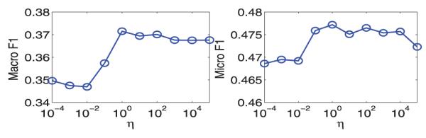
Sensitivity study of the parameter η in rASO: We study the relationship between the parameter η and the corresponding Micro F1 and Micro F1 obtained in rASO.

7.2 Evaluation of APG and BCD

We study the APG algorithm and the BCD method in terms of the convergence curves and the computation time (in seconds) by solving rASO with the hinge loss. For illustration, we set α = 1; β = 5; h = 2 in (8) and perform the webpages categorization task for the first three subcategories on the Arts data in the following experiments; for other parameters settings, we have similar observations. Note that APG and BCD are terminated if the change of the objective values in two successive iterations is smaller than 10⁻⁵ or the iteration number is larger than 5,000.

Convergence curves comparison

We randomly sample 2,000 samples (of feature dimensionality 17,973) from the Arts data for this experiment. We apply APG and BCD separately for solving (8) on the experimental data and record the obtained objective value in each of the iterations.

The experimental results are presented in Fig. 2. We can observe that APG requires about 15 iterations for convergence and its convergence curve is consistent with the theoretical convergence analysis of the APG algorithm [33], [34]. We can also observe that BCD converges very fast in practice; BCD converges within three iterations in this experiment (when the value of β is smaller than the value of α, BCD require a larger number of iterations for convergence).

Fig. 2.

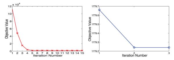
Convergence plots of APG (left plot) and BCD (right plot) for solving rASO with the hinge loss: We study the relationship between the objective value and the iteration number for attaining such a value.

Computation time comparison

We first consider the setting where the feature dimensionality is much larger than the sample size. We construct the first four subsets by randomly choosing {1, 000, 2, 000, 3, 000, 4, 000} samples (of dimensionality 17,973) from the Arts data, respectively. We apply APG and BCD on the constructed subsets and record the respective computation time in seconds. The experimental results are presented in Table 3. We observe that the computation time for APG and BCD increases with the increase of the sample size. We also observe that by using a fixed dimensionality, when the sample size is relatively small, for example, 1,000, APG requires more computation time than BCD; when the sample size is relatively large, for example, 2,000, 3,000, and 4,000, APG requires less computation time than BCD.

TABLE 3.

Computation Time (in Seconds) Comparison for APG and BCD

Sample Size	TimeAPG	TimeBCD	TimeAPG : TimeBCD
1000	43.96	17.86	2.4614
2000	118.69	140.64	0.8439
3000	280.69	685.18	0.4097
4000	480.79	1318.01	0.3648

We fix the feature dimensionality at 17,973 and vary the sample size in the set {1, 000, 2, 000, 3, 000, 4, 000}.

We then consider the setting where the sample size is much larger than the feature dimensionality. We construct the second four subsets by randomly choosing 3,000 samples from the Arts data and then reduce the feature dimensionality to {100, 200, 300, 400} via PCA. We apply APG and BCD on the constructed subsets and record the respective computation time. The experimental results are presented in Table 4. We can observe that the computation time for APG and BCD increases with the increase of the feature dimensionality. We can also observe that by using a fixed sample size, when the feature dimensionality is relatively small, for example, 100, APG requires less computation time than BCD; when the feature dimensionality is relatively large, for example 200, 300, and 400, APG requires more computation time than BCD.

TABLE 4.

Computation Time (in Seconds) Comparison for APG and BCD

Dimension	TimeAPG	TimeBCD	TimeAPG : TimeBCD
100	29.59	40.36	0.7332
200	60.90	67.28	0.9052
300	152.71	70.23	2.1744
400	212.80	85.47	2.4898

We fix the sample size at 3,000 and vary the dimensionality in the set {100, 200, 300, 400}.

7.3 Empirical Comparison of F₀ and F₂

We compare F₀ in (3) and F₂ in (8) in terms of the obtained optimal objective values. Since η is defined as η = β/α in Section 3, we vary the value of η by fixing α = 1, meanwhile varying β in the range [10³, 10², 10¹, 10⁰, 10⁻¹, 10⁻², 10⁻³]; we then record the obtained optimal objective values of F₀ and F₂, respectively, by using different combinations of α and β. We randomly choose 500 samples from the Arts data for this experiment. Note that the (locally) optimal objective value to F₀ is obtained via solving its equivalent form F₁ in (7). We solve both F₁ and F₂ using the BCD method and initialize the entries of the optimization variables from $\mathcal{N}(0,1)$.

The experimental results over random 20 repetitions are presented in Table 5. We observe that OBJ_F2 is always no larger than OBJ_F0; this is because F₂ is a relaxed version of F₁ (equivalently F₀) and has a larger domain set compared to F₀. We also observe that if σ_h/σ_h+1 > 1 + 1/η (corresponding to the first three columns in Table 5), OBJ_F0 is equal to OBJ_F2. The observations are consistent with the theoretical analysis in Theorem 6.1, that is, if σ_h/σ_h+1 > 1 + 1/η, F₀ and F₂ have the same optimal objective value and the optimal solution to F₀ can be recovered from F₂. Note that in general the condition σ_h/σ_h+1 > 1 + 1/η is satisfied when β is relatively larger than α.

TABLE 5.

Comparison of the Optimal Objective Values of F₀ in (3) and F₂ in (8) with Different Values of η

η = β/α	1000	100	10	1	0.1	0.01	0.001
1 + 1/η	1.001	1.01	1.1	2	11	101	1001
(σh/ση+1	1.23	1.25	1.34	1.75	3.07	13.79	89.49
OBJF0	52.78	52.65	51.37	40.73	22.15	5.95	0.69
OBJF2	52.78	52.65	51.37	40.71	20.73	4.11	0.41

We fix α = 1 and vary β in the range [10³, 10², 10¹, 10⁰, 10⁻¹, 10⁻², 10⁻³].

7.4 Automated Annotation of the Gene Expression Pattern Images

In this experiment, we apply rASO for the automated annotation of the Drosophila gene expression pattern images from the FlyExpress [36] database. We use SVM, ASO, cMTFL, and iSpLr as the baseline algorithms.

The Drosophila gene expression pattern images capture the spatial and temporal dynamics of gene expression and hence facilitate the explication of the gene functions, interactions, and networks during Drosophila embryogenesis [50], [51]. To provide text-based pattern searching, the gene expression pattern images are annotated manually using a structured controlled vocabulary (CV) in small groups, as shown in Fig. 3. Note that the CV terms are used to describe the differential anatomical features of the Drosophila embryos and the different stages of embryonic development; specifically, they provide specific terms for both finally developed embryonic structures and for all the developmental intermediates that precede those embryonic structures [52]. The annotation of CV terms is traditionally done manually by domain experts. However, with a rapidly increasing number of gene expression pattern images, it is desirable to design computational approaches to automate the CV annotation process.

Fig. 3.

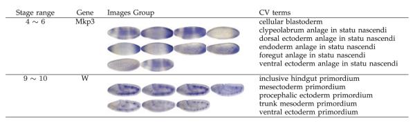
Illustration of image groups (from two stage ranges) and their associated controlled vocabulary terms.

We preprocess the Drosophila gene expression pattern images (of the standard size 128 × 320) following the procedures in [53]. The Drosophila images are from 16 specific stages, grouped into six stage ranges (1 ~ 3, 4 ~ 6, 7 ~ 8, 9 ~ 10, 11 ~ 12, 13 ~ 16). The image groups (based on the genes and the developmental stages) are labeled using the structured CV terms. Each image group is then represented by a feature vector based on the bag-of-words and the soft-assignment sparse coding schemes [53]. Due to the variation in morphology, shape, and position of various embryonic structures, we extract the scale-invariant feature transform (SIFT) features [54] from the gene expression images with the patch size set at 16 × 16 and the number of visual words in sparse coding set at 2,000. The first stage range only contains two CV terms and is not sufficient for constructing an experimental dataset. For other stage ranges, we construct the associated datasets by considering the top 10 CV terms or 20 CV terms appearing most frequently in the image groups.

For each constructed dataset, we focus on determining the relationship of the image groups and the CV terms. Since each image group may be associated with multiple CV terms and the CV terms are intrinsically related, we can formulate the image group annotation problems as a multitask learning problem. Note that classifying the image groups into one CV term is considered as a binary classification problem and hence we have multiple binary classification problems for each dataset (corresponding to one stage range). Specifically for each dataset, we randomly partition the data into training and test sets using the ratio 1:9. The parameters in the competing algorithms are tuned via threefold cross validation as in Section 7.1.

We report the averaged Macro F1 and Micro F1 over 10 random repetitions in Table 6 (10 CV terms) and Table 7 (20 CV terms), respectively. We observe that rASO performs the best or competitively compared to other algorithms on all subsets. This experiment demonstrates the effectiveness of rASO for the images annotation tasks in multitask learning setting as well as the effectiveness of the proposed regularizer in (4) for capturing the relationship of different CV terms of the gene expression images. We also observe that rASO outperforms ASO, which empirically shows the effectiveness of the regularizer in (4) for improving the performance among multiple tasks.

TABLE 6.

Performance Comparison of Competing Algorithms on the Gene Expression Pattern Images Annotation (10 CV Terms) in Terms of Macro F1 (Top Section) and Micro F1 (Bottom Section)

Stage Range (n, d, m)		4 ~ 6 (925, 2000, 10)	7 ~8 (797, 2000, 10)	9 ~ 10 (919, 2000, 10)	11 ~ 12 (1622, 2000, 10)	13 ~ 16 (2228, 2000, 20)
Macro F1	SVM	40.88 ± 0.49	46.73 ± 0.51	50.28 ± 0.65	59.82 ± 0.83	59.62 ± 0.94
	ASO	43.29 ± 0.46	48.82 ± 0.62	51.55 ± 0.90	62.15 ± 0.16	60.11 ± 0.32
	rASO	44.54 ± 0.79	50.59 ± 0.23	54.16 ± 0.75	63.43 ± 0.79	60.90 ± 0.77
	cMTFL	42.21 ± 0.69	48.17 ± 0.65	52.22 ± 0.35	62.17 ± 1.03	60.12 ± 0.27
	iSpLr	43.98 ± 1.23	49.19 ± 0.82	53.26 ± 1.19	62.73 ± 0.74	59.09 ± 1.02
Micro F1	SVM	42.05 ± 0.61	60.09 ± 0.78	60.57 ± 0.75	67.08 ± 0.99	65.95 ± 0.80
	ASO	45.89 ± 0.33	61.15 ± 0.57	63.01 ± 0.52	67.91 ± 0.51	66.53 ± 0.25
	rASO	47.34 ± 0.18	62.77 ± 0.61	64.37 ± 0.19	70.61 ± 1.21	67.13 ± 1.01
	cMTFL	46.07 ± 0.92	60.35 ± 0.31	63.22 ± 0.67	68.43 ± 0.25	67.35 ± 0.59
	iSpLr	46.91 ± 1.11	60.82 ± 1.07	63.34 ± 0.87	68.81 ± 0.95	66.90 ± 0.72

In the second row, n, d, and m denote sample size, dimension, and task numbers, respectively. In ASO and rASO, the shared feature dimensionality h is set as ⌊(m − 1)/5⌋ × 5.

TABLE 7.

Performance Comparison of the Competing Algorithms on the Gene Expression Pattern Images Annotation (20 CV Terms)

Stage Range (n, d, m)		4 ~ 6(1023, 2000, 20)	7 ~ 8(827, 2000, 20)	9 ~ 10(1015, 2000, 20)	11 ~ 12(1940, 2000, 20)	13 ~ 16(2476, 2000, 20)
Macro F1	SVM	29.47 ± 0.46	28.85 ± 0.62	30.03 ± 1.68	41.63 ± 0.58	40.80 ± 0.66
	ASO	30.33 ± 0.91	30.01 ± 0.67	32.22 ± 0.79	41.77 ± 1.43	40.98 ± 0.76
	rASO	31.01 ± 0.75	32.27 ± 0.91	35.01 ± 1.12	45.12 ± 0.21	43.81 ± 0.46
	cMTFL	30.66 ± 0.24	30.84 ± 0.39	34.13 ± 0.87	44.73 ± 0.49	43.13 ± 0.65
	iSpLr	30.08 ± 0.91	31.34 ± 1.01	34.89 ± 0.72	45.07 ± 0.77	42.90 ± 1.03
Micro F1	SVM	39.24 ± 0.82	55.40 ± 0.15	55.75 ± 0.70	58.33 ± 0.53	53.61 ± 0.36
	ASO	41.11 ± 0.32	57.72 ± 0.51	53.29 ± 0.21	61.77 ± 1.09	53.45 ± 0.92
	rASO	41.21 ± 1.24	59.34 ± 0.39	59.81 ± 0.33	63.25 ± 0.71	54.93 ± 0.78
	cMTFL	40.79 ± 0.31	58.39 ± 1.11	58.12 ± 0.84	61.22 ± 0.21	54.60 ± 0.62
	iSpLr	40.24 ± 0.69	58.87 ± 0.73	58.75 ± 0.81	62.90 ± 0.85	53.78 ± 0.87

7.5 Discussion

First, our experiments focus on the empirical comparison between ASO and rASO; the experimental results show that rASO usually outperforms ASO. Although we do not conduct empirical evaluation on iASO, we expect that iASO outperforms ASO while rASO outperforms iASO, due to several reasons: 1) iASO subsumes ASO as a special case: by choosing specific regularization parameters, iASO reduces to ASO. 2) rASO is a convex relaxation of iASO; in essence, rASO searches for a predictive model in a larger search space compared to iASO; hence, rASO may find a better predictive model. Note that in Section 2, we obtained iASO by adding an additional regularization to ASO, and then in Section 3 we obtained rASO by naturally relaxing the domain set of iASO to its convex hull.

Second, although our experiments focus on the application of rASO on classification problems, rASO can be naturally applied for regression problems. We apply rASO with the least square loss on a commonly used multitask regression benchmark data, the school data [8], in comparison with the boosted multitask learning algorithm proposed in [12]. Specifically, rASO achieves the explained variance at 37.3 ± 1.4, comparable to the best result 37.7 ± 1.2 attained by the boosted multitask learning algorithm in [12].

8 Conclusion and Future Work

In this paper, we present a multitask learning formulation (iASO) for learning a shared feature representation from multiple related tasks. Since iASO is nonconvex, we convert it into a relaxed convex formulation (rASO). In addition, we present a theoretical condition, under which rASO can find a globally optimal solution to iASO. We employ the BCD method and the APG method, respectively, to find the globally optimal solution to rASO; we also develop efficient algorithms to solve the key subproblems involved in BCD and APG. We have conducted experiments on the Yahoo datasets and the Drosophila gene expression pattern images datasets. The experimental results demonstrate the effectiveness and efficiency of the proposed algorithms and confirm our theoretical analysis. We are currently investigating how the solutions of rASO depend on the parameters involved in the formulation as well as their optimal value estimation. The rASO formulation shares some similarity with the multitask learning formulation using the trace norm regularization. We plan to examine their relationship in the future. We also plan to apply rASO to applications such as the automatic processing of biomedical texts for tagging the gene mentions [10].

Biography

Jianhui Chen received the PhD degree in computer science from Arizona State University in 2011. He is a research scientist with the Industrial Internet Analytics Lab of GE Global Research, San Ramon, California. His research interests include multitask learning, sparse learning, kernel learning, dimension reduction, and bioinformatics. He won the KDD best research paper award honorable mention in 2010.

Lei Tang received the BS degree from Fudan University, China and the PhD degree from Arizona State University in 2010. He is a research scientist in advertising sciences at Yahoo! Labs. His research interests include computational advertising, social computing, and data mining. He has published four book chapters and 25+ peer-reviewed papers in prestigious conferences and journals related to data mining and machine learning. His copresented tutorial on “Community Detection and Behavior Study for Social Computing” was featured in the IEEE International Conference on Social Computing, 2009. In September 2010, his book on Community Detection and Mining in Social Media was published by Morgan & Claypool publishers.

Jun Liu received the BS degree from the Nantong Institute of Technology (now Nantong University) in 2002, and the PhD degree from the Nanjing University of Aeronautics and Astronautics (NUAA) in November, 2007. During February 2008-February 2011, he was a postdoctoral researcher in the Biodesign Institute, Arizona State University. He is currently a research scientist at Siemens Corporate Research. His research interests include dimensionality reduction, sparse learning, and large-scale optimization. He has authored or coauthored more than 30 scientific papers.

Jieping Ye received the PhD degree in computer science from the University of Minnesota, Twin Cities, in 2005. He is an associate professor inf the Department of Computer Science and Engineering, Arizona State University. His research interests include machine learning, data mining, and biomedical informatics. He won the outstanding student paper award at ICML in 2004, the SCI Young Investigator of the Year Award at ASU in 2007, the SCI Researcher of the Year Award at ASU in 2009, the US National Science Foundation (NSF) CAREER Award in 2010, the KDD best research paper award honorable mention in 2010, and the KDD best research paper nomination in 2011. He is a member of the IEEE.

References

- [1].Bishop CM. Pattern Recognition and Machine Learning. Springer; 2006. [Google Scholar]
- [2].Hastie T, Tibshirani R, Friedman J. The Elements of Statistical Learning: Data Mining, Inference, and Prediction. Springer; 2009. [Google Scholar]
- [3].Caruana R. Multitask Learning. Machine Learning. 1997;vol. 28(no. 1):41–75. [Google Scholar]
- [4].Heisele B, Serre T, Pontil M, Vetter T, Poggio T. Categorization by Learning and Combining Object Parts. Proc. Advances in Neural Information Processing System. 2001 [Google Scholar]
- [5].Ando RK, Zhang T. A Framework for Learning Predictive Structures from Multiple Tasks and Unlabeled Data. J. Machine Learning Research. 2005;vol. 6:1817–1853. [Google Scholar]
- [6].Xue Y, Liao X, Carin L, Krishnapuram B. Multi-Task Learning for Classification with Dirichlet Process Priors. J. Machine Learning Research. 2007;vol. 8:35–63. [Google Scholar]
- [7].Yu S, Tresp V, Yu K. Robust Multi-Task Learning with t-Processes. Proc. Int’l Conf. Machine Learning. 2007 [Google Scholar]
- [8].Argyriou A, Evgeniou T, Pontil M. Convex Multi-Task Feature Learning. Machine Learning. 2008;vol. 73(no. 3):243–272. [Google Scholar]
- [9].Zhou J, Chen J, Ye J. MALSAR: Multi-tAsk Learning via StructurAl Regularization. Arizona State Univ.; 2012. [Google Scholar]
- [10].Ando RK. BioCreative II Gene Mention Tagging System at IBM Watson. Proc. Second BioCreative Challenge Evaluation Workshop.2007. [Google Scholar]
- [11].Bi J, Xiong T, Yu S, Dundar M, Rao RB. An Improved Multi-Task Learning Approach with Applications in Medical Diagnosis. Proc. European Conf. Machine Learning. 2008 [Google Scholar]
- [12].Chapelle O, Shivaswamy P, Vadrevu S, Weinberger K, Zhang Y, Tseng B. Boosted Multi-Task Learning. Machine Learning. 2011;vol. 85:149–173. [Google Scholar]
- [13].Quattoni A, Collins M, Darrell T. Learning Visual Representations Using Images with Captions. Proc. IEEE Conf. Computer Vision and Pattern Recognition. 2007 [Google Scholar]
- [14].Li J, Tian Y, Huang T, Gao W. Probabilistic Multi-Task Learning for Visual Saliency Estimation in Video. Int’l J. Computer Vision. 2010;vol. 90(no. 2):150–165. [Google Scholar]
- [15].Thrun S, O’Sullivan J. Discovering Structure in Multiple Learning Tasks: The TC Algorithm. Proc. Int’l Conf. Machine Learning. 1996 [Google Scholar]
- [16].Baxter J. A Model of Inductive Bias Learning. J. Artificial Intelligence Research. 2000;vol. 12:149–198. [Google Scholar]
- [17].Bakker B, Heskes T. Task Clustering and Gating for Bayesian Multitask Learning. J. Machine Learning Research. 2003;vol. 4:83–99. [Google Scholar]
- [18].Lawrence ND, Platt JC. Learning to Learn with the Informative Vector Machine. Proc. Int’l Conf. Machine Learning. 2004 [Google Scholar]
- [19].Schwaighofer A, Tresp V, Yu K. Learning Gaussian Process Kernels via Hierarchical Bayes. Proc. Advances in Neural Information Processing Systems. 2004 [Google Scholar]
- [20].Yu K, Tresp V, Schwaighofer A. Learning Gaussian Processes from Multiple Tasks. Proc. Int’l Conf. Machine Learning. 2005 [Google Scholar]
- [21].Zhang J, Ghahramani Z, Yang Y. Learning Multiple Related Tasks Using Latent Independent Component Analysis. Proc. Advances in Neural Information Processing System. 2005 [Google Scholar]
- [22].Jacob L, Bach F, Vert J-P. Clustered Multi-Task Learning: A Convex Formulation. Proc. Advances in Neural Information Processing System. 2008 [Google Scholar]
- [23].Evgeniou T, Pontil M. Regularized Multi-Task Learning. Proc. ACM SIGKDD Int’l Conf. Knowledge Discovery and Data Mining. 2004 [Google Scholar]
- [24].Evgeniou T, Micchelli CA, Pontil M. Learning Multiple Tasks with Kernel Methods. J. Machine Learning Research. 2005;vol. 6:615–637. [Google Scholar]
- [25].Jebara T. Multi-Task Feature and Kernel Selection for SVMs. Proc. Int’l Conf. Machine Learning. 2004 [Google Scholar]
- [26].Obozinski G, Taskar B, Jordan MI. Multi-Task Feature Selection. Proc. ICML Workshop Structural Knowledge Transfer for Machine Learning. 2006 [Google Scholar]
- [27].Argyriou A, Evgeniou T, Pontil M. Multi-Task Feature Learning. Proc. Advances in Neural Information Processing System. 2006 [Google Scholar]
- [28].Recht B, Fazel M, Parrilo PA. Guaranteed Minimum Rank Solutions to Linear Matrix Equations via Nuclear Norm Minimization. SIAM Rev. 2010;vol. 52(no. 3):471–501. [Google Scholar]
- [29].Ji S, Ye J. An Accelerated Gradient Method for Trace Norm Minimization. Proc. Int’l Conf. Machine Learning. 2009 [Google Scholar]
- [30].Pong TK, Tseng P, Ji S, Ye J. Trace Norm Regularization: Reformulations, Algorithms, and Multi-Task Learning. SIAM J. Optimization. 2009;vol. 20:3465–3489. [Google Scholar]
- [31].Zhou J, Chen J, Ye J. Clustered Multi-Task Learning via Alternating Structure Optimization. Proc. Advances in Neural Information Processing System. 2011 [PMC free article] [PubMed] [Google Scholar]
- [32].Bertsekas DP. Nonlinear Programming. Athena Scientific; 1999. [Google Scholar]
- [33].Nemirovski A. Efficient Methods in Convex Programming. Springer; 1995. [Google Scholar]
- [34].Nesterov Y. Introductory Lectures on Convex Programming. Kluwer Academic Publishers; 1998. [Google Scholar]
- [35].Ueda N, Saito K. Parametric Mixture Models for Multi-Labeled Text. Proc. Advances in Neural Information Processing System. 2002 [Google Scholar]
- [36].2012 http://www.flyexpress.net/
- [37].Overton ML, Womersley RS. Optimality Conditions and Duality Theory for Minimizing Sums of the Largest Eigenvalues of Symmetric Matrics. Math. Programming. 1993;vol. 62(nos. 1-3):321–357. [Google Scholar]
- [38].Boyd S, Vandenberghe L. Convex Optimization. Cambridge Univ. Press; 2004. [Google Scholar]
- [39].Argyriou A, Micchelli CA, Pontil M, Ying Y. A Spectral Regularization Framework for Multi-Task Structure Learning. Proc. Advances in Neural Information Processing System. 2007 [Google Scholar]
- [40].Golub GH, Van Loan CF. Matrix Computations. Johns Hopkins Univ. Press; 1996. [Google Scholar]
- [41].Sturm JF. Using SeDuMi 1.02, a MATLAB Toolbox for Optimization over Symmetric Cones. Optimization Methods and Software. 1999;vols. 11/12:625–653. [Google Scholar]
- [42].Chang C-C, Lin C-J. LIBSVM: A Library for Support Vector Machines. ACM Trans. Intelligent Systems and Technology. 2011;vol. 2:27:1–27:27. [Google Scholar]
- [43].Brucker P. An O(n) Algorithm for Quadratic Knapsack Problems. Operations Research Letters. 1984;vol. 3(no. 3):163–166. [Google Scholar]
- [44].Moreau J-J. Proximité et Dualité dans un Espace Hilbertien. Bull. Soc. Math. France. 1965;vol. 93:273–299. [Google Scholar]
- [45].Liu J, Ji S, Ye J. SLEP: Sparse Learning with Efficient Projections. Arizona State Univ.; 2009. [Google Scholar]
- [46].Bach F, Jenatton R, Mairal J, Obozinski G. Convex Optimization with Sparsity-Inducing Norms. In: Sra S, Nowozin S, Wright SJ, editors. Optimization for Machine Learning. MIT Press; 2011. [Google Scholar]
- [47].Chen J, Liu J, Ye J. Learning Incoherent Sparse and Low-Rank Patterns from Multiple Tasks. Proc. 16th ACM SIGKDD Int’l Conf. Knowledge Discovery and Data Mining; 2010. [DOI] [PMC free article] [PubMed] [Google Scholar]
- [48].Lewis DD, Yang Y, Rose TG, Li F. RCV1: A New Benchmark Collection for Text Categorization Research. J. Machine Learning Research. 2004;vol. 5:361–397. [Google Scholar]
- [49].Lewis DD. Evaluating Text Categorization. Proc. Speech and Natural Language Workshop. 1991 [Google Scholar]
- [50].Fowlkes CC, Hendriks CLL, Keränen SV, Weber GH, Rübel O, Huang M-Y, Chatoor S, DePace AH, Simirenko L, Henriquez C, Beaton A, Weiszmann R, Celniker S, Hamann B, Knowles DW, Biggin MD, Eisen MB, Malik J. A Quantitative Spatiotemporal Atlas of Gene Expression in the Drosophila Blastoderm. Cell. 2008;vol. 133(no. 2):364–374. doi: 10.1016/j.cell.2008.01.053. [DOI] [PubMed] [Google Scholar]
- [51].Lécuyer E, Yoshida H, Parthasarathy N, Alm C, Babak T, Cerovina T, Hughes TR, Tomancak P, Krause HM. Global Analysis of mRNA Localization Reveals a Prominent Role in Organizing Cellular Architecture and Function. Cell. 2007;vol. 131(no. 1):174–187. doi: 10.1016/j.cell.2007.08.003. [DOI] [PubMed] [Google Scholar]
- [52].Tomancak P, Beaton A, Weiszmann R, Kwan E, Shu S, Lewis SE, Richards S, Ashburner M, Hartenstein V, Celniker SE, Rubin GM. Systematic Determination of Patterns of Gene Expression during Drosophila Embryogenesis. Genome Biology. 2002;vol. 3(no. 12) doi: 10.1186/gb-2002-3-12-research0088. [DOI] [PMC free article] [PubMed] [Google Scholar]
- [53].Ji S, Yuan L, Li Y-X, Zhou Z-H, Kumar S, Ye J. Drosophila Gene Expression Pattern Annotation Using Sparse Features and Term-Term Interactions. Proc. 15th ACM SIGKDD Int’l Conf. Knowledge Discovery and Data Mining; 2009. [DOI] [PMC free article] [PubMed] [Google Scholar]
- [54].Lowe DG. Distinctive Image Features from Scale-Invariant Keypoints. Int’l J. Computer Vision. 2004;vol. 60(no. 2):91–110. [Google Scholar]
Associated Data
This section collects any data citations, data availability statements, or supplementary materials included in this article.