A Sample Selection Strategy to Boost the Statistical Power of Signature Detection in Cancer Expression Profile Studies

Abstract

In case-control profiling studies, increasing the sample size does not always improve statistical power because the variance may also be increased if samples are highly heterogeneous. For instance, tumor samples used for gene expression assay are often heterogeneous in terms of tissue composition or mechanism of progression, or both; however, such variation is rarely taken into account in expression profiles analysis. We use a prostate cancer prognosis study as an example to demonstrate that solely recruiting more patient samples may not increase power for biomarker detection at all. In response to the heterogeneity due to mixed tissue, we developed a sample selection strategy termed Stepwise Enrichment by which samples are systematically culled based on tumor content and analyzed with t-test to determine an optimal threshold for tissue percentage. The selected tissue-percentage threshold identified the most significant data by balancing the sample size and the sample homogeneity; therefore, the power is substantially increased for identifying the prognostic biomarkers in prostate tumor epithelium cells as well as in prostate stroma cells. This strategy can be generally applied to profiling studies where the level of sample heterogeneity can be measured or estimated.

INTRODUCTION

Expression profiling technologies measuring RNA or proteins have become more popular for research on diseases because it can survey many thousands of genes simultaneously and shed light on novel genes or biological pathways that are related to disease and disease progression [1-4]. Usually, samples are collected for at least two groups; a case group (for example, patients that have relapsed with prostate cancer after prostatectomy) as well as a control group (for example, patients that did not relapse after prostatectomy). Altered gene expression levels between the case group and the control group are identified with differential analysis methods. Here we will concentrate on an example using array analysis of RNA levels where standard tests have been developed, such as regulated-t test [5], SAM [6], and Bayesian Regression Model [7]. The selected genes are likely to be related to the disease and can be validated by follow-up studies. Due to the substantial decrease in the cost of expression analysis procedures over the last few years, especially the introduction of high-throughput sequencing methods, one can include a large number of samples in experiments and the chance of identifying disease-associated genes is, thereby, expected to be increased. However, experience indicates that this may not be always the case. For example, several independent research groups carried out similar studies to identify genes related to breast cancer progression, each involving hundreds of breast cancer samples [8-15]. However, there was very little overlap in terms of gene identity among the gene sets identified in these independent studies. A similar result was reported in a meta-analysis of prostate cancer profiling data [16]. This is very common in the tumor marker literature which has numerous examples of assays that produce inconsistent results when data from different laboratories are compared [17, 18]. This inconsistency among the gene composition of the profiles is likely due in part to the multiple paths taken to cancer and metastases, heterogeneity among different parts of the diseased tissue, and underlying biological variability in cancer progression including reversible alterations. Another speculation for the disparity between different laboratories in the gene sets that correlate with disease outcome is that the expression levels of many genes are weakly correlated to each other, yielding a large pool of genes weakly associated with disease outcome; individual studies will identify subsets of these genes, with little overlap in terms of gene identity. Such non-overlap would be expected if the number of genes that have a weak correlation with outcome is large. Other factors include variability in tissue handling and RNA extraction in different laboratories [19], or systematic bias between the compared groups tends to produce positive results that do not reflect an underlying reality and are not reproducible [20, 21].

One of our recent studies on prostate cancer suggested that heterogeneity of samples, for example the variable cell composition across prostate samples, might also dramatically contribute to variation in gene expression [3]. The prostatectomy tissues are composed of three major cell components: tumor epithelial cells, stroma, and epithelium of benign prostate hyperplasia (BPH). The content of each type of cell differs among samples. Sample heterogeneity may severely limit the conclusions that can be made about the specificity of expression profiles. Without controlling for variation caused by heterogeneity of samples and patients, solely increasing patient sample size will not help identify reliable expression signatures that are associated with the disease. Laser Capture Microdissection (LCM) has been introduced for gleaning purer tissue. However, LCM when applied to multiple cell types for numerous samples is potentially impractical, arduous, and it is difficult to routinely prepare high quality RNA. Moreover, it is desirable to make good use of the enormous amount of banked data collected prior to LCM, especially because the accompanying long-term clinical follow-up is vital for a disease that progresses slowly in most patients.

Here, we provide a case study to demonstrate that controlling for cell composition heterogeneity is as important as increasing sample size in microarray and expression profiles experiment design. Moreover, we present a sample selection strategy termed Stepwise Enrichment for prostate cancer profiling studies in which heterogeneity in tissue constitution is commonly an impacting factor. By this strategy, samples are systematically culled to reveal the optimal threshold for tissue percentage that reaches a balance between the sample size and the sample homogeneity, maximizing the number and significance of candidate biomarkers. The approach extends a recent in silico approach which estimates cell-type distributions for any prostate sample based on multigene signatures that are invariant with tumor surgical pathology parameters of Gleason and stage [22]. The Stepwise Enrichment approach can be generally applied to profiling studies where any important aspect of sample heterogeneity can be measured. We show that when cell-type heterogeneity is controlled, the number and significance of expression changes associated with the outcome of prostate cancer can be increased. We applied the new method to one of our expression data set with known cell-type percentage information. The outcome-associated biomarkers in tumor cells as well as in stroma cells (tumor microenvironment) have been identified and compared. The majority of the tumor signatures are different from the stroma signatures. Moreover, when cell-type heterogeneity is controlled, a second source of heterogeneity among expression changes in tumor component specifically associated with poor outcome prostate cancer is “unmasked”. The potential for understanding this important class of genes is discussed.

MATERIALS AND METHODS

Our prostate cancer dataset, which has been used for demonstration in this study, is publically available at Gene Expression Omnibus (GEO) with access number GSE8218 [3]. This dataset consists of 136 samples from 82 patients who went through prostatectomy. The gene expression was measured by using Affymetrix U133A chips. For each sample used in the microarray assay, the percentages of the three major cell components (tumor epithelial cells, stroma cells and BPH epithelial cells) were estimated by pathologists. Among these 82 patients, 45 experienced disease relapse (case group), 33 did not (control group) and the remaining 4 were unknown. The 136 samples include 65 tumor-bearing samples and 71 non-tumorous samples. For tumor signature analysis, we only considered the data for 65 tumor-bearing samples (tumor content ranging from 2% to 80%) with known outcomes, whereas, for stroma signature analysis, we only used the data for 65 tumor-free samples (stroma content ranging from 40% to 100%) with known outcomes.

The paper in which the original data were presented [3], dealt with the heterogeneous samples via using a multiple-linear-regression (MLR) model by which the observed Affymetrix gene expression values are described as linear combination of the contribution from different types of cells [3, 22]. By fitting the MLR model with the expression data, the patient outcome data, and the cell-type percentage data (pathological estimation), relapse-associated genes in individual cell type (e.g., tumor cells and stroma cells) can be accurately identified. We analyzed the data of the 65 tumor-bearing samples with this MLR analysis and detected 310 relapse-associated genes that are specifically expressed in tumor (adjusted p-value < 0.01). We assumed these tumor prognostic genes are ‘real’ and therefore used them to evaluate the tumor signatures obtained by t-tests (See DISCUSSION).

A dataset of 200 samples was simulated. First, we randomly assigned the 200 samples into either the case group (denoted by 1) or the control group (denoted by 0) with equal chances. This was realized by generating 200 binary variables (1 or 0) with probabilities 0.5 versus 0.5. For each sample, the percentages of three cell types were simulated as follows. We let cell type 3 (BPH) be the minority cell which takes up to 10% volume in tissues; thus, we first generated the percentage of cell type 3 ( X₃ ) from uniform distribution U(0, 0.1). We then generated the percentage of cell type 1 ( X₁ for tumor) from U(0, 1 - X₃ ), and the percentage of cell type 2 ( X₂ for stroma) is therefore 1 - X₁ - X₃. Note that the cell-type distribution used for guiding the simulation was estimated from the real prostate cancer dataset [3]. For each sample, we simulated expression data for 1000 gene as follows. We let genes 1 to 60 have altered expression in cell type 1 between case and control. The differences in terms of expression for genes 1 to 20, genes 21 to 40 and genes 41 to 60 are set to 0.5, 1.0 and 2.0, respectively. The same setting was used for generating differentially expressed genes for cell type 2 (genes 61 to 120). Due to the small load for cell type 3, we assume that the difference between case and control in cell type 3 is undetectable, so we did not simulate differentially expressed genes for cell type 3.

The statistical methods applied in this study include Linear Models for Microarray Data (LIMMA) [5], survival analysis (R routine by Terry Therneau), Multiple Linear Regression (MLR) fitting implemented in our previous study [3, 22], a novel score to evaluate agreement between two gene lists, and an Empirical Concordance Evaluation approach developed in this study (See RESULTS). Above statistical analyses as well as simulating random variables from Bernoulli distribution and uniform distribution were carried out in R (version 2.9.0.) environment (http://www.r-project.org/). Hierarchical clustering was carried out by using software Genesis [23].

RESULTS

Analysis of prostate cancer data

We first carried out a differential analysis between case and control groups (relapse versus non-relapse) on the 65 tumor-bearing samples using the moderated t-test implemented in the LIMMA package in R [5]. We identified 204 genes which showed altered expression between the relapse and non-relapse groups based on B statistics which is defined as log-transformed posterior odds that any particular gene is differentially expressed. Any gene with B > 0 is claimed as significant by LIMMA. The same criterion of B > 0 was applied to the gene selection by the subsequent t-tests using the LIMMA.

To explore the impact of changing sample size on statistical power, we did an experiment involving a random subsample selection strategy. Specifically, we randomly and independently selected a subset of 10, 15, …, 60 samples from the data with replacement and carried out differential expression analysis by t-test on each subgroup of samples, respectively. This random process was iterated 100 times. The average numbers of genes identified by 100 random subsets at each particular sample size are depicted by the red curve in Figure 1(a). The detection rate monotonically increased as the size of the random resample went up (red curve in Figure 1(a)). However, compared to the 204 genes identified when all 65 tumor samples were used, the numbers of genes identified by 95 or more of 100 resamples of each particular sample size (blue curve) were 0 if the sample size was no more than 45 patients. In addition, none of the 310 MLR-derived genes were rediscovered if the sample size was less than 45 (green curve in Figure 1(a)).

Fig. 1.

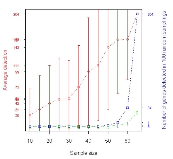
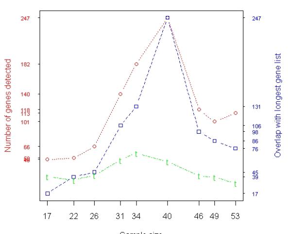
Analysis of prostate cancer data. A total of 65 samples (31 relapses and 34 non-relapses) were profiled by Affymetrix microarrays. (a) Results of t-test based on averaging 100 random experiments in which subsets of samples were randomly selected from the entire population (65 samples). The red curve with error bars represents the average numbers of genes detected in 100 resamples at each individual sample size represented by the x-axis. The blue curve represents the numbers of genes identified by 95 or more of 100 resamples of each particular size that were also in the list of 204 genes identified when all 65 samples were used. The green curve represents the overlap between the genes identified by 95 or more of 100 resamples of each particular size and the 310 tumor genes identified with MLR using all the 65 samples. (b) Relapse-associated genes in tumor identified by t-test when samples were selected based on T cutoff (Stepwise Enrichment). The x-axis shows that there were 17 samples with ≥ 60% tumor, 22 samples with ≥ 55% tumor, …, and 53 samples with ≥ 20% tumor. The red curves indicate the numbers of genes identified at each particular size. The blue curves represent the overlap between the reference gene list and other gene lists. The reference gene list is the gene list identified when 40 samples were used. The green curve illustrates the overlap between each gene lists and the 310 tumor genes identified with MLR using all the 65 samples.

In contrast to the random selection strategy, we developed a new sample selection strategy termed “Stepwise Enrichment”. In this process, samples were selected on the basis of tumor cell con-tent to form quartiles. Specifically, we used a series of tumor percentage cutoffs (T ≥ 20%, T ≥ 25%, …, T ≥ 55%, T ≥ 60%) for sample selection, where T stands for the percentage of tumor component in samples. Therefore, there were 17 samples with ≥ 60% tumor, 22 samples with ≥ 55% tumor, …, and 53 samples with ≥ 20% tumor. The numbers of genes identified by t-test at each particular size are summarized in Figure 1(b), with maximum detection of 247 probe sets (reference gene list) when 40 of the most tumor-enriched samples were analyzed. Note the longest gene list (247 Affymetrix probe sets) identified by t-test in Stepwise Enrichment strategy is called reference gene list and it indicates the optimal threshold for tissue percentage that reveals the most significant data. The detailed information about these 247 probe sets is given in supplement Table S1. Of the 310 MLR-derived tumor genes, 57 were also identified when 34 of the most tumor-enriched samples (with ≥ 40% tumor) were used for t-test (see green peak in Figure 1(b)). We then calculated the empirical p-values for the 57 overlapping genes between the 310 MLR-derived tumor genes and the 182 tumor genes identified by t-test at sample size 34. Let count = 0. From about 22,000 genes, we randomly selected two gene lists of length 310 and 182, respectively. If the overlap of the two randomly selected gene lists is equal or greater than 57 (observed overlap between the 310 MLR-derived genes and the 182 genes identified by t-test), we let the count increase by 1. We repeated this process 10,000 times and the p-value of the observed overlap is calculated as

$$p=\mathit{count}∕10000.$$

The calculation showed that the p-value for tumor overlapping genes was ≤ 0.0001. Thus, the 182 genes identified by the 34 samples, which were adjacent to the reference gene list (red peak) disclosed by Stepwise Enrichment, were strongly supported by MLR.

We also compared genes identified with different subsets of samples selected using T cutoffs in Stepwise Enrichment. In Table 1, the diagonal entries (shaded) are the numbers of gene identified with each particular subset of samples. The off-diagonal entries are the numbers of common genes identified with two different subsets of samples. To evaluate the association/concordance among these gene lists detected with different subsets of samples, we created a score ρ denoted as:

$$\rho =1-{\left[\frac{l(A\backslash B)}{l\left(A\right)}\times \frac{l(B\backslash A)}{l\left(B\right)}\right]}^{\frac{1}{2}},$$ (1)

where A and B are two mathematical sets representing two different gene lists, A \ B denotes all elements that are members of set A but not members of set B, l ( A ) is a function that calculates the number of elements in set A. Note l (∅) = 0 , where ∅ is an empty set. We utilized the ρ score to assess the agreement between two gene lists. If two gene lists are identical or one list is a sub-list of the other, ρ = 1. On the other hand, if two gene lists are totally different, ρ = 0 . The heatmap based on ρ values among these gene lists is depicted in Figure 2(a). We also tracked the change of variations for the measurement of ~22,000 probe sets when sample size was increased by continuously adding low-tumor-content samples. By using a box plot, we summarized the distributions of variances for the measurement of ~22,000 probe sets for relapsed cases (yellow boxes) and non-relapsed cases (orange boxes) at each particular size (Figure 2(b)). It appeared that the median variance of ~22,000 probe sets for both relapse and non-relapse groups tended to increase if samples became more heterogeneous. Another interesting observation in Figure 2(b) is that the variances for relapsed cases are higher than those for non-relapsed cases.

Table 1.

Comparison between gene lists identified by t-test with different subsets of samples selected using a series of cutoffs based on the percentage of tumor in each sample (Stepwise Enrichment). There were 17 samples with ≥ 60% tumor, 22 samples with ≥ 55% tumor, …, and 53 samples with ≥ 20% tumor. The diagonal entries (shaded) are the numbers of gene identified with each particular subset of samples. The off-diagonal entries are the numbers of common genes identified with two different subsets of samples.

	N=53	N=49	N=46	N=40	N=34	N=31	N=26	N=22	N=17
N=53	113	63	74	76	46	42	21	21	4
N=49	63	101	80	86	59	50	25	23	6
N=46	74	80	118	98	61	53	27	23	6
N=40	76	86	98	247	131	106	45	39	17
N=34	46	59	61	131	182	122	50	38	18
N=31	42	50	53	106	122	140	51	35	16
N=26	21	25	27	45	50	51	66	34	16
N=22	21	23	23	39	38	35	34	50	17
N=17	4	6	6	17	18	16	16	17	48

Fig. 2.

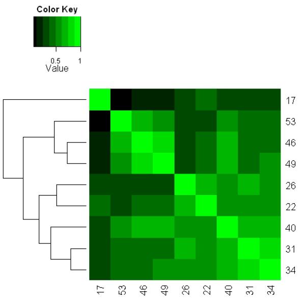
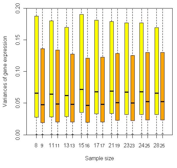
Comparison between gene lists identified by t-test with different subsets selected from 65 prostate cancer samples using a series of T cutoffs (Stepwise Enrichment). (a) Heat map showing association or concordance between the gene lists based on pair-wise scores (see formula (1) in RESULTS). The numbers in each row/column represent the numbers of samples selected using different T cutoffs, i.e., there were 17 samples with ≥ 60% tumor, 22 samples with ≥ 55% tumor, …, and 53 samples with ≥ 20% tumor. The rows/columns were clustered based on the similarity among the gene lists. If two gene lists are identical or one list is a sub-list of the other, ρ =1. On the other hand, if two gene lists are totally different, ρ = 0. (b) Box-plot showing the distribution of variances for the measurement of ~22,000 probe sets among different subsets of samples. The relapse cases and the non-relapse cases are treated separately due to the hypothesized biological variation between these two groups. Yellow/orange boxes describe the distribution of probe variances among the relapsed/non-relapsed cases at each particular size. The black band near the middle of each box represents the median variance in that distribution. The numbers below yellow/orange boxes represent the numbers of the relapsed/non-relapsed cases selected for t-test at each particular size. For example, 17 samples (8 relapses and 9 non-relapses) were selected by T ≥ 60%.

We repeated the analysis for the samples which are free of tumor cells. The new Stepwise Enrichment method identified the best subset of tumor-free samples based on which a total of 440 probe sets were found to have altered expression between relapsed cases and non-relapsed cases. In contrast to the new method, only 282 probe sets were detected to be differentially expressed if all the tumor-free samples were used for analysis (regular approach), with 207 in common with the 440 probe sets identified with the new method. In addition, there were only 8 common probe sets between the 247 tumor signatures and the 440 stroma signatures. The various lists of biomarkers identified in the study are listed in the supplemental Table S1.

Simulation study

To demonstrate the advantages of the new sample selection method of Stepwise Enrichment, a simulation was carried out (See METERIALS AND METHODS for the details of generating the data). In the same way as done with the analysis of real expression data, we randomly selected a subset of 40, 50, …, 180, 190 samples from the 200 simulated samples and carried out differential expression analysis using t-test. The sensitivity, specificity and false discovery rate had been logged at each particular sample size. Such analysis was repeated 100 times and the average operating characteristic is summarized in Figure 3(a).

Fig. 3.

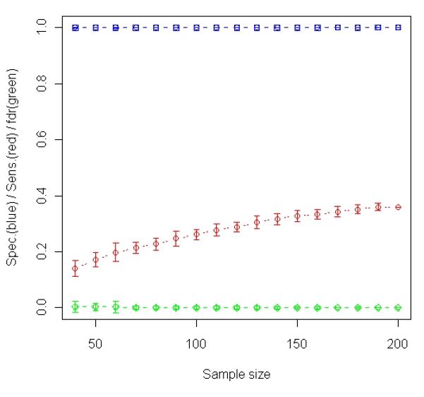
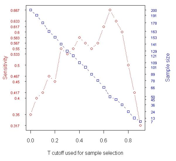
Analysis of simulated data. A total 1000 gene expression levels were simulated for each of 200 samples (100 relapses and 100 non-relapses). Among the 1000 genes, 60 were simulated to be relapse-associated signatures in tumor and the other 60 were simulated to be relapse-associated signatures in stroma. The simulated tumor percentage for these 200 samples varies from 1% to 98%. (a) Results of t-test based on averaging 100 random experiments in which subsets of samples were randomly selected from the entire population (200 samples). The curves in blue, red and green with error bars represent specificity, sensitivity and false discovery rate, respectively, at each particular sample size. (b) The changes in Sensitivity (red curve) and number of samples selected for t-test (blue curve) when different T cutoffs were used for sample selection (Stepwise Enrichment).

We then selected samples by stepwise enriching type 1 cell. Specifically, we included samples with X₁ ≥ k% (k = 0, 5, …, 85, 90) in t-test, and then identified genes that are differentially expressed in cell type 1 between case and control. With varying cutoff, the number of samples included in analysis and the sensitivity or power achieved by these subsets of samples are summarized in Figure 3(b).

Finally, we analyzed the simulated data with MLR, as summarized in Table 2. As expected, MLR analysis accurately identified relapse-associated genes in tumor and stroma. This result suggested that genes identified by t-test could be validated with MLR-derived genes as we did for real prostate cancer analysis.

Table 2.

Operating characteristics for MLR analysis of cyber-data. A total 1000 gene expression levels were simulated for each of 200 samples (100 relapses and 100 non-relapses). Among the 1000 genes, 60 were simulated to be relapse-associated signatures in tumor and the other 60 were simulated to be relapse-associated signatures in stroma. The simulated tumor percentage for these 200 samples varies from 1% to 98%.

	Sensitivity	Specificity
Tumor signatures	93.3%	96.2%
Stroma signatures	98.3%	96.1%

DISCUSSION

In this study, we investigated the relationship between statistical power and number of samples in t-test when two types of sample selection schemes were compared: random sampling and the selection by Stepwise Enrichment based on tumor content. Nevertheless, the MLR analysis [3, 22] was more desirable than t-test because (i) using the percentage data as covariates for regression analysis is more accurate than selecting samples based on the percentage cutoff, and (ii) all samples are effectively used for calculation leading to increased power. This was supported by the results of a simulation study, in which the best sensitivity achieved by t-test was 66.7% (Figure 3(b)), while the sensitivity for the MLR analysis was 93.3% (Table 2). In addition, there have been attempts to tackle the problem of expression deconvolution using MLR-like approaches [24 - 26]. However, precise measures of cell components are not commonly available for many studies where a t-test still applies. Here, we developed a strategy to select most significant samples for t-test based on tissue percentage. Available bioinformatics applications (e.g., [22]) may be applied to approximate cell constitution if pathological cell-type distribution data are missing, and this therefore facilitates the application of the sample selection protocol proposed in the study. Since genes identified with MLR are close to reality, we attempted to validate results of the t-test by MLR result in the current study.

For the tumor analysis where samples were randomly selected, the detection rate increased as the size of the random resample monotonically went up (red curve in Figure 1(a)). However, compared to the 204 genes identified when all 65 patient samples were used, the numbers of genes identified by 95 or more of 100 resamples of each particular patient population size (blue curve) were 0 if the sample size was no more than 45 patients, indicating inconsistent findings for individual subset of samples. Note that common genes with the entire data set were observed when sample size was over 50 (right end of Figure 1(a)) but only because each resampling included such a large fraction of the full dataset, leading to a less variable result that in a random process. Moreover, none of the 310 MLR-identified tumor genes were detected if the sample size was less than 45 (green curve in Figure 1(a)). The similar results were obtained in stroma analysis (data not shown).

The results obtained using Stepwise Enrichment analyses were dramatically better. For tumor analysis, nine subsets of samples were selected by using a series of tumor percentage cutoffs. In Figure 1(b) the maximum detection (247 genes) occurred when the 40 most tumor-rich samples (T ≥ 35%) were included in the analysis. There were substantial overlap (>67%, blue curve) among the detected genes at this point with other gene lists identified near this point (sample sizes 31 to 49), indicating consistent discovery among these assays. Therefore, we conclude that these 40 samples with T ≥ 35%, which is indicated by the red peak, represent the most significant data identified by the new Stepwise Enrichment approach. In addition, the overlap with the MLR result was much improved for the experiments based on the new sample selection strategy (green curve in Figure 1(b)). The green curve (overlaps with MLR result) showed a bell-shaped pattern; the optimal cutoff occurred at some point in the middle where the balance between sample size and homogeneity was reached. Moreover, the empirical p-value for the overlap between the two gene lists identified by MLR and t-test (sample size = 34 in Figure 1(b)) was ≤ 0.0001, suggesting a significant concordance between t-test analysis based on Stepwise Enrichment strategy and the MLR analysis. The similar results were obtained in stroma analysis (data not shown).

In Figure 2(a), we used a heatmap based on ρ (see formula (1) in RESULTS) to explore the association/concordance among the 9 tumor gene lists identified by the 9 subsets of samples represented by x-axis in Figure 1(b). The rows (and columns) in the heatmap are clustered based on similarity between gene lists to test our hypothesis that samples with similar levels of homogeneity are likely to produce comparable gene lists. There appear to be three major clusters for these 9 gene lists, i.e., {cluster 1: N = 17}, {cluster 2: N = 53, 46, and 49}, and {cluster 3: N = 26, 22, 40, 31, 34}. Cluster 3 represents samples mainly enriched with tumor, whereas cluster 2 represents the sum of samples in cluster 3 and samples that contain much less tumor. The subsets included in each cluster have similar sizes, i.e., those subsets contain many same samples selected based on tumor content; therefore, they are of similar levels of homogeneity. The result supported our hypothesis and indicated a significant increase in variance given the increased heterogeneity of the samples. Cluster 1 represents the case when only 17 samples are selected (T ≥ 60%). Due to the limited power when these 17 samples were analyzed, we only detected 48 genes, some of which might be spurious owing to the relatively small sample size. Interestingly, there was a fair agreement between cluster 1 and 3 ($\stackrel{‒}{\rho }$ = 0.268 ); while there was little agreement between cluster 1 and 2 ($\stackrel{‒}{\rho }$ = 0.048 ). The disagreement between cluster 2 versus clusters 1 and 3 may be ascribed to the inclusion of low-tumor-content samples that substantially increased the sample heterogeneity. Again, a suspicion is raised for the gene lists identified for cluster 2 in which most samples were included in the analysis. This concurred with the result shown in Figure 2(b), where the median variance of about 22,000 probe sets for both relapse and non-relapse groups tended to increase if samples became more heterogeneous. In addition, we observed in Figure 2(b) that the variances for relapsed cases are always higher than those for non-relapsed cases. One possible explanation is that the disease recurrence can be caused by multiple biological mechanisms which involve different pathways and gene sets, leading to even larger variances in gene expression specifically among relapsed samples. The substantial increase in variances for the relapsed cases may indicate that the relapsed cases may be even more heterogeneous with respect to gene expression subclasses and not merely composed of a single class of expression changes that are normally distributed. Indeed, unsupervised clustering of the relapsed cases reveals a suggestion of subclasses within the relapse cases (Figure S1). In Figure S1, a heatmap based on the clustering revealed two subgroups of relapsed cases. A Kaplan-Meier analysis showed that these two sub-populations have slightly different outcomes in terms of progression free survival (p-value = 0.09 in Log-rank test, Figure S2), suggesting two different mechanisms for prostate cancer progression. If and when larger sample sizes are available for relapse cases and increased time of follow-up, these two or more subgroups may be more confidently distinguished. Thus the control of cell-type heterogeneity may help pinpoint gene expression changes that are correlated with poor outcome and further provide for subclassification. The similar results were obtained in stroma analysis (data not shown).

We then analyzed the 247 tumor signatures that have been identified by the new approach using the pathway software MetaCore (GeneGo Inc.). The result indicated that many of these 247 tumor genes are associated with transcriptional factors, such as p53 and SP1, which play crucial roles in cancer development and progression (Figure S3). In addition, 32 out of these 247 genes are relevant to prostatic neoplasia in men. We also analyzed the 440 stroma signatures using MetaCore. Similarly, many of these genes are associated with SP1 and HNF4 which is a nuclear receptor protein (Figure S4). Moreover, 187 out of these 440 genes are relevant to prostate gland. Interestingly, there are only 8 common genes between the 247 tumor signatures and 440 stroma signatures, indicating the specificity of biomarkers in different cell types. The sum of the evidence suggested that the new method indeed identified potential biomarkers in tumor and stroma with diagnostic and/or prognostic values for prostate cancer.

We also generated a simulated set of prostate cancer data to determine if t-test based on the samples selected by the new Stepwise Enrichment approach produces more reliable results than t-test based on entire data set or any randomly selected subset. In the simulation, we looked at 200 samples with mixtures of three cell types. We looked at 1000 genes of which 60 were set to be differentially expressed in tumor. Appropriate noise was added to all the data. Similar setting for simulation study has been utilized in the literature [7, 27]. We investigated the relationship between power and number of samples when two types of sample selection schemes were applied to the simulated data: random sampling (Figure 3(a)) and the selection by Stepwise Enrichment (Figure 3(b)). For random sampling, the sensitivity or power went up as sample size increased (Figure 3(a)); however, the detection rate was limited with a maximum of 36.1%. In Figure 3(b), the maximum sensitivity or power is 66.7% which is much higher than any figures attained by randomly selected samples in Figure 3(a). In addition, the maximum sensitivity or power achieved when X₁ ≥ 65%, neither too small nor too large in terms of the content of cell type 1. If the selected cutoff is too small, most samples will be included. This compares to the observation in the random experiment when sample size is close to the upper limit (see Figure 3(a)). In this case, the variation caused by mixed tissue is likely to impair detection power as we hypothesized. However, if the selected cutoff is too large, too few samples will be included in the analysis, leading to a reduced power. For example, if we use X₁ ≥ 90% for sample selection, only 9 samples (5 controls and 4 cases) were selected. The sensitivity or power in this situation is only 43%. This is similar to the observation in prostate cancer data analysis which showed a bending-down detection curve when sample size is near 0 (Figure 1(b)). The bell-shaped curve in red of Figure 3(b) indicated that there is a trade off between sample size and level of homogeneity among samples. Both factors could positively contribute to power, i.e., increase of either size or homogeneity of samples may improve the analysis. Nevertheless, these two factors do not benefit from each other in this example because they cannot be escalated simultaneously if samples are highly heterogeneous. Plausible homogeneity is only achievable when imperfect samples are discarded while increased variability is inevitable when all samples are included in assay. This is very similar to the roles of type I and type II errors in statistical tests. The results indicate that carefully selecting samples from a resource using our proposed strategy is superior to utilizing all available samples indiscriminately. In respect of study planning, this is in agreement with Simon et al.’s remarks [28] in which they discussed the level of evidence based on types of samples used for discovery studies.

By simulation as well as by using real prostate cancer data, we demonstrated that increasing sample size will not necessarily boost power if offsetting factors, such as sample heterogeneity (cell composition is the example in the current study), are not effectively controlled. Rather, samples can be systematically culled by the new Stepwise Enrichment strategy to reveal the optimal threshold for tissue percentage that will yield the most significant data and significantly increase detection power. This strategy can be generally applied to profiling studies where the level of sample heterogeneity can be measured or estimated.

References

- [1].Blalock EM, Geddes JW, Chen KC, Porter NM, Markesbery WR, Landfield PW. Incipient alzheimer’s disease: Microarray correlation analyses reveal major transcriptional and tumor suppressor responses. Proc Natl Acad Sci USA. 2004;101(7):2173–2178. doi: 10.1073/pnas.0308512100. [DOI] [PMC free article] [PubMed] [Google Scholar]
- [2].Schena M, Shalon D, Davis RW, Brown PO. Quantitative monitoring of gene-expression patterns with a complementary-dna microarray. Science. 1995;270(5235):467–470. doi: 10.1126/science.270.5235.467. [DOI] [PubMed] [Google Scholar]
- [3].Stuart RO, Wachsman W, Berry CC, Wang-Rodriguez J, Wasserman L, Klacansky I, Masys D, Arden K, Goodison S, McClelland M, Wang Y, Sawyers A, Kalcheva I, Tarin D, Mercola D. In silico dissection of cell-type-associated patterns of gene expression in prostate cancer. Proc Natl Acad Sci USA. 2004;101(2):615–620. doi: 10.1073/pnas.2536479100. [DOI] [PMC free article] [PubMed] [Google Scholar]
- [4].Koziol JA, Feng AC, Jia Z, Wang Y, Goodison S, McClelland M, Mercola D. The wisdom of the commons: ensemble tree classifiers for prostate cancer prognosis. Bioinformatics. 2009;25(1):54–60. doi: 10.1093/bioinformatics/btn354. [DOI] [PMC free article] [PubMed] [Google Scholar]
- [5].Smyth GK. Linear models and empirical Bayes methods for assessing differential expression in microarray experiments. Stat Appl Genet Mo B. 2004;3 doi: 10.2202/1544-6115.1027. Article 3. [DOI] [PubMed] [Google Scholar]
- [6].Tusher VG, Tibshirani R, Chu G. Significance analysis of microarrays applied to the ionizing radiation response. Proc Natl Acad Sci USA. 2001;98(9):5116–5121. doi: 10.1073/pnas.091062498. [DOI] [PMC free article] [PubMed] [Google Scholar]
- [7].Jia Z, Xu S. Bayesian mixture model analysis for detecting differentially expressed genes. Int J Plant Genomics. 2008 doi: 10.1155/2008/892927. Article ID 892927, 12 pages. [DOI] [PMC free article] [PubMed] [Google Scholar]
- [8].Fan C, Oh DS, Wessels L, Weigelt B, Nuyten DSA, Nobel AB, van’t Veer LJ, Perou CM. Concordance among gene-expression-based predictors for breast cancer. New Engl J Med. 2006;355(6):560–569. doi: 10.1056/NEJMoa052933. [DOI] [PubMed] [Google Scholar]
- [9].Chang HY, Sneddon JB, Alizadeh AA, Sood R, West RB, Montgomery K, Chi JT, van de Rijn M, Botstein D, Brown PO. Gene expression signature of fibroblast serum response predicts human cancer progression: Similarities between tumors and wounds. Plos Biology. 2004;2(2):206–214. doi: 10.1371/journal.pbio.0020007. [DOI] [PMC free article] [PubMed] [Google Scholar]
- [10].Paik S, Shak S, Tang G, Kim C, Baker J, Cronin M, Baehner FL, Walker MG, Watson D, Park T, Hiller W, Fisher ER, Wickerham DL, Bryant J, Wolmark N. A multigene assay to predict recurrence of tamoxifen-treated, node-negative breast cancer. New Engl J Med. 2004;351(27):2817–2826. doi: 10.1056/NEJMoa041588. [DOI] [PubMed] [Google Scholar]
- [11].Sorlie T, Perou CM, Tibshirani R, Aas T, Geisler S, Johnsen H, Hastie T, Eisen MB, van de Rijn M, Jeffrey SS, Thorsen T, Quist H, Matese JC, Brown PO, Botstein D, Eystein Lønning P, Børresen-Dale AL. Gene expression patterns of breast carcinomas distinguish tumor subclasses with clinical implications. Proc Natl Acad Sci USA. 2001;98(19):10869–10874. doi: 10.1073/pnas.191367098. [DOI] [PMC free article] [PubMed] [Google Scholar]
- [12].Sorlie T, Tibshirani R, Parker J, Hastie T, Marron JS, Nobel A, Deng S, Johnsen H, Pesich R, Geisler S, Demeter J, Perou CM, Lønning PE, Brown PO, Børresen-Dale AL, Botstein D. Repeated observation of breast tumor subtypes in independent gene expression data sets. Proc Natl Acad Sci USA. 2003;100(14):8418–8423. doi: 10.1073/pnas.0932692100. [DOI] [PMC free article] [PubMed] [Google Scholar]
- [13].Sotiriou C, Neo SY, McShane LM, Korn EL, Long PM, Jazaeri A, Martiat P, Fox SB, Harris AL, Liu ET. Breast cancer classification and prognosis based on gene expression profiles from a population-based study. Proc Natl Acad Sci USA. 2003;100(18):10393–10398. doi: 10.1073/pnas.1732912100. [DOI] [PMC free article] [PubMed] [Google Scholar]
- [14].van de Vijver MJ, He YD, van ’t Veer LJ, Dai H, Hart AA, Voskuil DW, Schreiber GJ, Peterse JL, Roberts C, Marton MJ, Parrish M, Atsma D, Witteveen A, Glas A, Delahaye L, van der Velde T, Bartelink H, Rodenhuis S, Rutgers ET, Friend SH, Bernards R. A gene-expression signature as a predictor of survival in breast cancer. New Engl J Med. 2002;347(25):1999–2009. doi: 10.1056/NEJMoa021967. [DOI] [PubMed] [Google Scholar]
- [15].van’t Veer LJ, Dai HY, van de Vijver MJ, He YD, Hart AA, Mao M, Peterse HL, van der Kooy K, Marton MJ, Witteveen AT, Schreiber GJ, Kerkhoven RM, Roberts C, Linsley PS, Bernards R, Friend SH. Gene expression profiling predicts clinical outcome of breast cancer. Nature. 2002;415(6871):530–536. doi: 10.1038/415530a. [DOI] [PubMed] [Google Scholar]
- [16].Michiels S, Koscielny S, Hill C. Prediction of cancer outcome with microarrays: a multiple random validation strategy. The Lancet. 2005;365(9458):488–492. doi: 10.1016/S0140-6736(05)17866-0. [DOI] [PubMed] [Google Scholar]
- [17].McShane LM, Aamodt R, Cordon-Cardo C, Cote R, Faraggi D, Fradet Y, Grossman HB, Peng A, Taube SE, Waldman FM. Reproducibility of p53 immunohistochemistry in bladder tumors. National Cancer Institute, Bladder Tumor Marker Network. Clin Cancer Res. 2000;6(5):1854–1864. [PubMed] [Google Scholar]
- [18].Sweep CG, Geurts-Moespot J. EORTC external quality assurance program for ER and PgR measurements: trial 1998/1999. European Organisation for Research and Treatment of Cancer. Int J Biol Markers. 2000;15(1):62–69. doi: 10.1177/172460080001500112. [DOI] [PubMed] [Google Scholar]
- [19].Dobbin KK, Beer DG, Meyerson M, Yeatman TJ, Gerald WL, Jacobson JW, Conley B, Buetow KH, Heiskanen M, Simon RM, Minna JD, Girard L, Misek DE, Taylor JM, Hanash S, Naoki K, Hayes DN, Ladd-Acosta C, Enkemann SA, Viale A, Giordano TJ. Interlaboratory comparability study of cancer gene expression analysis using oligonucleotide microarrays. Clin Cancer Res. 2005;11:565–572. [PubMed] [Google Scholar]
- [20].Ransohoff DF. The process to discover and develop biomarkers for cancer: a work in progress. J Natl Cancer Inst. 2008;100(20):1419–1420. doi: 10.1093/jnci/djn339. [DOI] [PubMed] [Google Scholar]
- [21].Ransohoff DF, Gourlay ML. Sources of bias in specimens for research about molecular markers for cancer. J Clin Oncol. 2010;28(4):698–704. doi: 10.1200/JCO.2009.25.6065. [DOI] [PMC free article] [PubMed] [Google Scholar]
- [22].Wang Y, Xia X, Jia Z, Sawyers A, Yao H, Wang-Rodriquez J, Mercola D, McClelland M. In silico estimates of tissue components in surgical samples based on expression profiling data. Cancer Research. 2010;70(16):6448–6455. doi: 10.1158/0008-5472.CAN-10-0021. [DOI] [PMC free article] [PubMed] [Google Scholar]
- [23].Sturn A, Quackenbush J, Trajanoski Z. Genesis: cluster analysis of microarray data. Bioinformatics. 2002;18(1):207–208. doi: 10.1093/bioinformatics/18.1.207. [DOI] [PubMed] [Google Scholar]
- [24].Clarke J, Seo P, Clarke B. Statistical expression deconvolution from mixed tissue samples. Bioinformatics. 2010;26(8):1043–1049. doi: 10.1093/bioinformatics/btq097. [DOI] [PMC free article] [PubMed] [Google Scholar]
- [25].Lu P, Nakorchevskiy A, Marcotte E. Expression deconvolution: A reinterpretation of DNA microarray data reveals dynamic changes in cell populations. Proc Natl Acad Sci USA. 2003;100(18):10370–10375. doi: 10.1073/pnas.1832361100. [DOI] [PMC free article] [PubMed] [Google Scholar]
- [26].Wang M, Master S, Chodosh L. Computational expression deconvolution in a complex mammalian organ. BMC Bioinformatics. 2006;7:328. doi: 10.1186/1471-2105-7-328. [DOI] [PMC free article] [PubMed] [Google Scholar]
- [27].Jia Z, Xu S. Mapping quantitative trait loci for expression abundance. Genetics. 2007;176:611–623. doi: 10.1534/genetics.106.065599. [DOI] [PMC free article] [PubMed] [Google Scholar]
- [28].Simon RM, Paik S, Hayes DF. Use of archived specimens in evaluation of prognostic and predictive biomarkers. J Natl Cancer Inst. 2009;101(21):1446–1452. doi: 10.1093/jnci/djp335. [DOI] [PMC free article] [PubMed] [Google Scholar]
Associated Data
This section collects any data citations, data availability statements, or supplementary materials included in this article.