Optimal whole-body PET scanner configurations for different volumes of LSO scintillator: a simulation study

Abstract

The axial field of view (AFOV) of the current generation of clinical whole-body PET scanners range from 15–22 cm, which limits sensitivity and renders applications such as whole-body dynamic imaging, or imaging of very low activities in whole-body cellular tracking studies, almost impossible. Generally, extending the AFOV significantly increases the sensitivity and count-rate performance. However, extending the AFOV while maintaining detector thickness has significant cost implications. In addition, random coincidences, detector dead time, and object attenuation may reduce scanner performance as the AFOV increases. In this paper, we use Monte Carlo simulations to find the optimal scanner geometry (i.e. AFOV, detector thickness and acceptance angle) based on count-rate performance for a range of scintillator volumes ranging from 10 to 90 l with detector thickness varying from 5 to 20 mm. We compare the results to the performance of a scanner based on the current Siemens Biograph mCT geometry and electronics. Our simulation models were developed based on individual components of the Siemens Biograph mCT and were validated against experimental data using the NEMA NU-2 2007 count-rate protocol. In the study, noise-equivalent count rate (NECR) was computed as a function of maximum ring difference (i.e. acceptance angle) and activity concentration using a 27 cm diameter, 200 cm uniformly filled cylindrical phantom for each scanner configuration. To reduce the effect of random coincidences, we implemented a variable coincidence time window based on the length of the lines of response, which increased NECR performance up to 10% compared to using a static coincidence time window for scanners with large maximum ring difference values. For a given scintillator volume, the optimal configuration results in modest count-rate performance gains of up to 16% compared to the shortest AFOV scanner with the thickest detectors. However, the longest AFOV of approximately 2 m with 20 mm thick detectors resulted in performance gains of 25–31 times higher NECR relative to the current Siemens Biograph mCT scanner configuration.

1. Introduction

In current clinical whole-body PET scanners, the axial field of view (AFOV) is approximately 15–22 cm (Bettinardi et al 2004, Surti and Karp 2004, Jakoby et al 2011). A long AFOV scanner that could image a large fraction of the body at one time would significantly increase sensitivity and would open the door to new applications, such as whole-body parametric imaging of pharmacological kinetics and systemic imaging of radiolabeled stem cell progenitor cell populations.

With current limited AFOV scanners, parametric PET imaging is difficult for several reasons. Although arterial blood sampling is currently the gold standard for parametric PET imaging (Cook et al 1999), it requires frequent arterial blood sampling to generate time-activity curves and plasma input function parameters (De Geus-Oei et al 2006). In addition, such studies are currently limited to single organs that can fit into the field of view (e.g. brain and heart, Lortie et al 2007, Mourik et al 2009) unless significant compromises in temporal resolution are accepted (Karakatsanis et al 2011).

A long AFOV scanner is always capable of imaging the heart or a large blood vessel along with the region of interest. This allows the performance of parametric imaging through image data alone, thus providing a reasonable substitute for arterial blood sampling. A large AFOV scanner could then determine pharmacokinetic parameters for multiple organs simultaneously, which could be highly advantageous in the determination of efficacy and likely side-effects early in the drug discovery pipeline. As with arterial blood sampling, the early time points of the acquired time-activity curves may have significant noise, even with a highly sensitive scanner.

A second limitation of current clinical whole-body PET scanners is due to the fact a large portion of the body lies outside of the AFOV, which results in a low effective detection efficiency of about 0.2–0.3% (Cherry 2006). Low sensitivity negatively impacts quantitative parametric imaging as it enforces practical limits to temporal sampling at early time-points and results in poor signal-to-noise ratio (SNR) in time-activity curves, which renders the determination of kinetic parameters an ill-posed problem. At the same time, low sensitivity also limits the utility of PET as a tool in future applications such as monitoring of therapeutic stem-cell trafficking (Zhang et al 2007), which may require the ability to detect very small amounts of radiotracer in parts of the body that may not be known in advance. In addition, poor scanner sensitivity impacts current clinical PET applications in ways including those listed below:

• low SNR in reconstructed images

• relatively high absorbed dose for each imaging study

• poor spatial resolution due to filtering requirements

• long scan times, which leads to patient motion

• low patient throughput.

At first glance, it is obvious that the sensitivity for true coincidence events can be maximized by extending the AFOV to completely cover any subject of interest with thick scintillator detectors (Cherry 2006). Simulation studies of various long AFOV PET scanner geometries have shown significant sensitivity improvements (Badawi et al 2000; Couceiro et al 2007, Wong et al 2007, Eriksson et al 2007, Eriksson et al 2008, MacDonald et al 2011), which addresses the limitations on whole-body kinetic parameter estimation discussed above. However, there are a few trade-offs that result from such a configuration.

First, a long AFOV scanner may have a much greater singles event rate, which increases the random event rate and places a significant burden on detector electronics. Second, long AFOV scanners have large acceptance angles, which require wider a coincidence timing window to accommodate the time of flight for long lines of response (LORs) between two distant detectors. A wider coincidence timing window also increases the random event rate. Without great care in scanner design, these factors may reduce count-rate performance and also negate the benefits of a long AFOV scanner for many applications. Two extended AFOV scanners have been built, the Siemens P39–5H with a 53 cm AFOV (Conti et al 2006) and the Hamamatsu SHR-92000, a 68.5 cm AFOV scanner (Watanabe et al 2004). Both systems demonstrated significant improvements in sensitivity, but due to electronics and readout limitations in the first case and the use of a slow scintillator in the second, performance at higher count-rates was only marginally improved compared to current PET scanners.

Three other factors may also impact performance of a large AFOV scanner. In human imaging, LORs at large acceptance angles typically encounter a significant amount of object attenuation, which acts to decrease effective sensitivity and may increase the probability of detecting scattered coincidences. In addition, thick detectors provide greater detection efficiency, but also lead to degradation of spatial resolution due to depth of interaction (DOI) blurring. For large AFOV scanners, the DOI blurring in the axial direction has the potential to be a major factor. Conversely, time-of-flight (TOF) capability may provide added benefit in large AFOV scanners, since the improvements in image SNR are expected to be greatest for LORs that pass through long distances of tissue (Karp et al 2008, Fakhri et al 2011).

A critical consideration for large AFOV scanners is cost. While acquisition electronics have become cheaper (and faster) in recent years, the same cannot be said for PET scintillators, particularly lutetium oxyorthosilicate (LSO) or its derivatives, which are materials of choice for most fully 3D PET systems today. Cheaper materials (e.g. bismuth germanate (BGO) or gadolinium silicate (GSO)) could be considered for a long AFOV scanner, but their use leads to a compromise in either timing performance or sensitivity. To save costs, one could build a large AFOV scanner using the same amount of LSO scintillator material by reducing the detector thickness. However, the trade-off between reduced detector sensitivity and improved solid-angle coverage is not known.

In this paper, we determine the optimal scanner geometry (i.e. AFOV, detector thickness, and acceptance angle) for a range of scintillator volumes (approximately 10 to 90 l) using Monte Carlo simulations. The simulation model is validated against measured data from the Siemens mCT scanner (Jakoby et al 2011). The noise equivalent count rate (NECR) is used as a benchmark to characterize the global SNR and act as a surrogate for system-level image quality (Wollenweber et al 2003). The NECR value is determined as a function of activity concentration and maximum ring difference (i.e. acceptance angle) inside any given AFOV scanner geometry. This approach has the advantage of simplicity and keeps the computational cost manageable. However, we note that NECR is not able to account for changes in spatial resolution due to DOI effects or the impact of TOF capability. At the same time, noise equivalent counts (NEC) has not been explicitly validated as a surrogate for image SNR for scanners with large acceptance angles.

To maximize count-rate performance in extended AFOV scanners, control of the random coincidence event rate is crucial. The coincidence time window in current systems is calculated based on the longest time of flight difference and the coincidence timing resolution. The randoms event rate is proportional to the coincidence time window and singles event rate of the system. As the sensitivity increases, the probability of multiple single events falling into a time window also increases. At the same time, all possible prompt coincidences are recorded in most modern scanners, which also causes the randoms event rate to increase dramatically due to multiple coincidences as well (i.e. three single events may lead to three prompt coincidences, four single events may lead to six prompt coincidences, etc). To reduce the impact of randoms, we explore using a variable coincidence time window that is a function of ring difference. This is an approach related an idea proposed by Conti (2007) to use a variable coincidence time window for each line of response, determined by the maximum useful time of flight obtained from a concurrent CT image of the object.

2. Materials and methods

2.1. Photon tracking Monte Carlo simulations

All of the photon tracking Monte Carlo simulations were performed using the Geant4 Application for Tomographic Emission (GATE) version 5.0p1 described by Jan et al (2004). GATE is a simulation tool with validated physics models for PET imaging. GATE is used to simulate positron emission and annihilation, model gamma ray photon absorption and scatter in objects and LSO scintillator material. In-house code is used for frontend detector pulse processing, electronic multiplexing and coincidence generation.

2.2. Validation against Siemens Biograph mCT

We first validate our simulation setup by modeling the Siemens Biograph mCT and comparing the NEMA NU 2–2007 scatter fraction, count-rates and NECR results from simulated data against experimental data. The experimental results were obtained from measurements performed at the University of California-Los Angeles.

2.2.1. Scanner properties (Jakoby et al 2011)

The basic unit of the Siemens Biograph mCT is the detector module, which consists of a 13 × 13 grid of LSO crystals that sits on top of a plastic material (modeled as plastic in GATE) to position the detector on the gantry. Each crystal is 4 × 4 × 20 mm³ and the block cross section approximately 54 × 54 mm² (Conti and Rothfuss 2010). The scanner has 48 detector blocks per ring with 4 rings (192 blocks in total). In the transaxial direction, opposing detector modules are separated by 849 mm. The exact geometry and dimensions were provided by Siemens through private communication.

The scanner is sandwiched by two lead end shields. A voxelized CT image of the patient bed and NEMA cylinder was used. Although the bed uses carbon fiber, the exact material composition and density were unknown. We modeled the bed as carbon material with a density of 1.4 g cc⁻¹. The density of carbon was linearly extrapolated from the Hounsfield units of air and polyethylene in the CT image.

2.2.2. Block detector/front-end model

All events interacting in each crystal of a detector block are recorded and time sorted. Starting with the initial event, the detector triggers only if the total energy of events in the block within a 300 ps window is greater than 150 keV (Binkly et al 2002). To determine the total trigger energy, events occurring within the trigger time period are blurred with an energy dependent energy resolution based on experimental data published by Kapusta et al (2005) to approximately model the non-proportional response of LSO. The detector requires a period of time for the trigger to reset and process events again, which was set to a proprietary value found in the Siemens electronic configuration. The time stamp of each final qualified event is blurred by 375 ps frontend timing resolution and digitized using a 78 ps clock period when the detector triggers (Conti 2009, Jakoby et al 2011).

After the detector block triggers, the signal is integrated for approximately 100–120 ns (Eriksson et al 2008), depending on when the trigger occurs with respect to the clock cycle. All events that occur within the integration window are used to determine a final position and energy of a single event. First, each event within the integration window is assumed to generate a light pulse, which is modeled as a single exponential function. The integral of the exponential function from the time stamp to the end of the integration window determines the integrated energy of the event. Each exponential function is calibrated so integrated energy equals the total energy of the event when the whole integration window is used. A perfect baseline offset for the detector is assumed, so the exponential tails past the integration window are extinguished.

The total integrated energy is blurred assuming an energy resolution of 11.7% at 511 keV (Jakoby et al 2011). A qualified single is accepted if the final energy value falls between 435–650 keV (Jakoby et al 2011). The position of the qualified single is determined by an energy weighted centroid of all events.

LSO background is modeled using a ¹⁷⁶Lu source confined to the detector crystals in the GATE simulation. In the Siemens Biograph mCT, the total LSO background contributes approximately 1.1M qualified singles per second without activity in the field of view (Jakoby et al 2011). In the simulation, the ¹⁷⁶Lu source was set to an activity concentration of 330 Bq/cc of LSO to match the singles rate measured on the scanner.

2.2.3. Block detector multiplexing model

A group of four independent detector blocks (1 transaxial × 4 axial) form a bucket (48 buckets total). Two individual buckets are multiplexed together to form one output (24 total outputs). The first and only qualified single between two multiplexed buckets is accepted every 80 ns, which is the system master clock period (Eriksson et al 2008).

2.2.4. Standard time window coincidence processing algorithm

A time ordered list of up to 24 qualified singles (24 total multiplexed outputs) is generated every 80 ns for coincidence processing. Each qualified single on the list is temporarily paired with every possible qualified single that occurs subsequently, which allows the system to accept all possible prompt coincidences. The temporary coincidence pairs are then filtered with criteria shown in table 1 to determine if they are valid prompt coincidences. At the same time, randoms are estimated through a delayed time window algorithm based on the proprietary Siemens electronic acquisition system.

Table 1.

Criteria to determine valid coincidence event for Siemens Biograph mCT.

Parameter	Value
Coincidence time window (time difference)	≤4.1 ns
Crystal ring difference	≤49
Bucket index difference	≤9 (70 cm FOV)

2.2.5. Modified NEMA data processing

A significant number of prompts are required in each sinogram slice to reduce the variability in estimating the number of counts at the boundaries of the 40 mm strip described in the NEMA protocol. To reduce the simulation time needed to accumulate a significant number of counts, we merge all sinogram slices into one before performing the NEMA analysis to determine the scatter fraction, count rates, and NECR. The modified method is also applied to the experimental data to compare the simulation results against.

2.3. Scintillator volume optimization study

The goal is to determine the optimal detector thickness and the axial length (adding detector modules axially) to maximize NECR. Peak NECR is determined as a function of activity concentration and maximum accepted ring difference for a uniformly filled cylinder with ¹⁸F in aqueous solution. The cylinder is 27 cm in diameter and 200 cm in length with a mass (114.5 kg) approximately comparable to a human male of the same height. At the same time, we compare the NECR performance between the standard and variable time window coincidence processing algorithm (described below). During standard coincidence processing, the time window was calculated and set globally for each maximum ring difference value.

We use the Siemens Biograph mCT model described in section 2.2 as the reference for the study with a few modifications. First, the time stamp is digitized using a 10 ps clock period to accommodate fine increments of maximum ring difference values. Second, the detector block multiplexing is eliminated, so all qualified singles are accepted for coincidence processing. Third, the patient bed is modeled using three rectangular sheets (200 cm in length, 9 mm thick) of carbon (density of 1.4 g cc⁻¹). Lastly, the detector block configurations for each set of scintillator volumes are shown in table 2.

Table 2.

The matrix below describes all of the scanner configurations simulated. Each row represents the number of axial detector blocks and each column represents the total scintillator volume (in liters). The detector thickness (in units of mm) for each configuration is shown for each row and column.

	Total scintillator volume (liters)
Number of axial detector blocks	10.38	15.58	20.77	31.15	41.53	62.3	83.07	93.45
4	20
6	13.33	20
8	10	15	20
10	8	12	16
12	6.66	10	13.33	20
16	5	7.5	10	15	20
24		5	6.66	10	13.33	20
32			5	7.5	10	15	20
36				6.67	8.89	13.33	17.78	20

2.3.1. Variable time window coincidence processing algorithm

A time ordered list of qualified singles from every detector block is generated every 200 ns for coincidence processing. The same coincidence processing algorithm described in section 2.2.4 is used to determine prompt and delay window (100 ns delay) coincidences. However, the time window is a function of the ring difference between each possible pair of single events in coincidence. If the time difference between these two single events is less than the calculated time window, the coincidence is accepted. This effort is made to minimize the random coincidence rate in an approach broadly similar to that described by Conti (2007). The time window is calculated using equation (1) below:

$$\tau (R)=\frac{\sqrt{T^2+{(R·W)}^2}}{c}+3·P,$$ (1)

where R is the ring difference, T is the transaxial field of view (70 cm), W is the axial crystal pitch, P is the coincidence timing resolution (530 ps), and c is the speed of light. The largest possible ring difference for a scanner configuration is equal to the total number of axial crystal elements in addition to the gaps between detector blocks.

2.3.2. Data processing

The NECR and scatter fraction are calculated using the following formulae:

$$\mathrm{NECR}=\frac{T^2}{T+S+k·R}$$ (2)

$$\mathrm{Scatter\; fraction}=\frac{T}{T+S},$$ (3)

where T, S, and R are the trues, scatter and randoms coincidence rate respectively. The scatter fraction is calculated using the true and scatter coincidence events that are labeled directly in the simulation. Note that this computation is not directly comparable to the NEMA standard scatter fraction reported by manufacturers, although previous work suggests that results are likely to be close (Badawi et al 2000, Ferrero et al 2011). The k value is set to 1, on the assumption that a low variance estimate of the randoms is used. At the same time, only LORs that pass through the cylindrical phantom are counted, which means the radial displacement in the sinogram of LORs must be less than or equal to the radius of the cylindrical phantom.

The NECR plot for each scanner configuration is fitted with a seventh order polynomial function from which peak NECR, optimal maximum ring difference, and optimal activity concentration is determined.

3. Results

3.1. Validation

Figure 1 shows the total qualified singles rate after multiplexing at the bucket level. Figure 2 shows the NEMA NU 2–2007 trues + scatter, randoms, NECR count rate, and scatter fraction results. Table 3 shows the error for between each set of curves using the measured values on the scanner as the reference. The error was calculated without including the last value where an unmodeled phenomenon in the Siemens Biograph mCT occurs, possibly due to the saturation of current in the photomultiplier tubes at very high singles rate (Casey 2011). For the count-rate curves, the maximum fractional error occurs at lowest activity concentration values, while the minimum fractional error occurs near the highest activity concentration values. The simulated results for total qualified singles, trues and scatters rate overestimates the experimental results by approximately 5–7%. The simulated randoms rate is proportional to the simulated qualified single rate squared. As expected, the simulated randoms rate overestimates the experimental randoms rate by approximately 12%.

Figure 1.

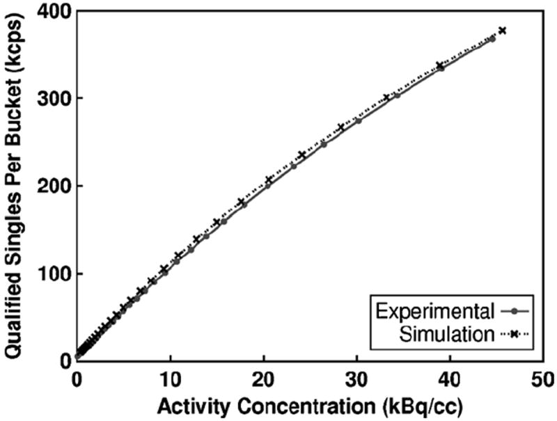
The total qualified singles rate at each bucket after multiplexing for the simulated model and actual Siemens Biograph mCT using the 20 cm diameter NEMA count-rate cylindrical phantom.

Figure 2.

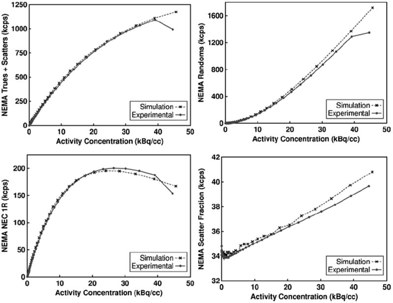
The simulated model and measured results for the 20 cm diameter NEMA count-rate cylindrical phantom on the Siemens Biograph mCT. The trues+scatters (top left), randoms (top right), NEC 1R (bottom left) and scatter fraction (bottom right) were calculated using the NEMA NU 2–2007 method.

Table 3.

Error between each set of count-rate curves in figures 1 and 2.

	Average error	Minimum error		Maximum error
	Error (%)	Error (%)	Activity (kBq/cc)	Error (%)	Activity (kBq/cc)
Singles	6.41	0.87	45.61	10.06	0.39
Trues+scatters	6.03	1.24	28.31	8.82	0.73
Randoms	12.33	6.96	38.93	20.15	0.45
NEC 1R	4.24	−4.2	38.93	8.58	0.73
Scatter fraction	0.73	−0.3	0.39	2.57	45.61

3.2. Scintillator volume optimization study

3.2.1. Maximum ring difference and coincidence time window optimization

Two examples of NECR plots as a function of maximum ring difference and activity concentration using the standard coincidence time window method are shown in figure 3. For each maximum ring difference value, a static time window calculated using equation (1) is set globally to process all coincidence events. The shape of the plot on the left is fairly typical for scanners with an AFOV ≪ 700 mm, while the plot on the right is typical for scanners with an AFOV ≫ 700 mm. NECR is optimized by including all possible LORs between detector rings for the shorter AFOV scanners. However, NECR is optimized by rejecting large oblique angle LORs for longer AFOV scanners due to two effects. First, the wider coincidence time window to accommodate long LORs results in a greater random coincidence rate. Second, the attenuation of LORs at large acceptance angles reduces the yield of true coincidence events counted as the maximum ring difference increases, while scatter and random coincidence events are essentially unaffected.

Figure 3.

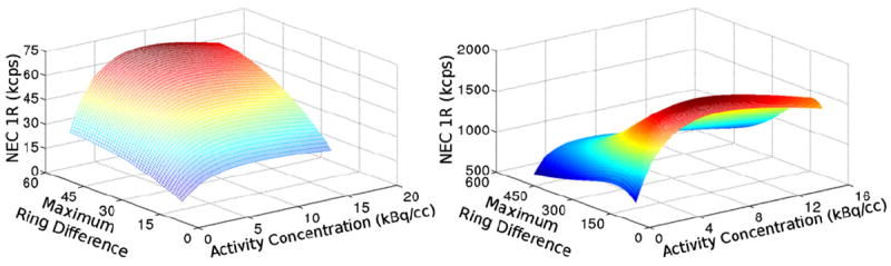
NEC 1R plotted as a function of maximum ring difference and activity concentration for the ~10 l—4 axial blocks mCT-like scanner (left) and the ~90 l—36 axial blocks scanner (right).

The longest AFOV scanners benefit from the variable coincidence timing window method the most, which modestly improved peak NECR performance by approximately 10% with respect to NECR performance using the standard coincidence time window. Minimal benefits of using a variable coincidence time window were seen for short AFOV scanners.

For scanners with an AFOV less than ~500–600 mm, the optimal ring difference is equal to the maximum ring difference. However, for long AFOV scanners, no advantage is found in increasing the ring difference corresponding to an axial extent greater than ~700 mm. NECR performance does not vary greatly near the optimal point, and for the 670 mm scanner, 90% of peak NECR can be obtained by accepting a ring difference of ~400 mm. However, NECR is drastically penalized when operating at ring differences significantly greater than the optimum. Unsurprisingly, the optimal ring difference to reach peak NECR for a given activity concentration decreases as the activity concentration increases.

3.2.2. Detector thickness and axial field of view optimization

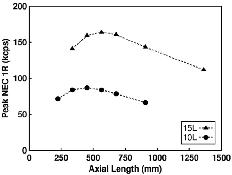
The sensitivity tradeoff between detector thickness and AFOV can be optimized, but this optimization yields diminishing gains in count-rate performance for larger scintillator volumes. In figure 4, the optimal configuration to maximize NECR for ~10 and ~15 l of scintillator volume is shown, where the optimal AFOV of 450 and 560 mm corresponds to a detector thickness of 10 and 12 mm respectively. The optimal configuration yields an increase in count-rate performance of approximately 16% and 11% relative to the smallest AFOV (with 20 mm thick detectors) for ~10 and ~15 l of scintillator volume respectively. The results shown are in general agreement with results by Surti et al (2011).

Figure 4.

Peak NEC 1R results using the variable coincidence timing window method for the set of scanners with 10 and 15 l of scintillator volume.

The peak NECR and NECR at 1 kBq/cc (equivalent to an injected dose of 5.64 mCi, assuming a 1 h uptake time and 20% excretion) for all of the scanner configurations are shown in figure 5. The NECR gains relative to the ~10 l (four axial blocks, mCT-like) scanner are also shown. The 20 l (eight axial blocks) scanner shows a peak NECR gain factor of 3.17, while the ~90 l (36 axial blocks) scanner shows a peak NECR gain factor of 25.81. At 1 kBq/cc, the relative gains in NECR are larger–3.58 for the 20 l and 31.6 for the ~90 l scanners. For the larger scintillator volumes ranging from ~60–90 l, the absolute peak NECR performance was not found, since we limited the maximum AFOV of the simulated scanners to 36 axial blocks (205 cm)

Figure 5.

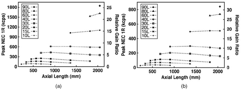
Peak NEC 1R results using the variable coincidence timing window method (a). Peak NEC 1R results using the variable coincidence timing window method at 1 kBq/cc activity concentration (b). The relative gain ratio is calculated by normalizing the NEC 1R values with respect to the 10 l (mCT-like) scanner result.

The optimal activity concentration at peak NECR is plotted as a function of axial length for scanners with 20 mm thick detectors in figure 6. The optimal activity concentration decreases initially, but increases again for AFOVs greater than ~1000 mm. The increase at large AFOVs can be explained by the fact that the scanner covers a greater portion of the phantom, and randoms due to activity outside the field of view start to decrease. However, the greater AFOV coverage increases the number of true coincidences accepted, which allows the scanner to reach peak NECR at a greater activity concentration. The activity concentration for peak NECR is larger than typically used for ¹⁸F based clinical imaging, but could be relevant for studies employing ¹³N, ¹¹C, or ¹⁵O-labeled radiotracers.

Figure 6.

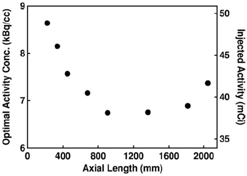
Optimal activity concentration where peak NECR occurs is plotted as a function of axial length for scanners with 20 mm thick detector blocks. Injected activity is calculated assuming a half life of 109.7 min, 20% excretion, and 1 h uptake.

At the optimal activity concentration for the scanners with 20 mm thick detectors, we quantify bandwidth requirements for different parts of the system. In figure 7, we plot the maximum block singles rate and the total system singles rate at the optimal activity concentration for peak NECR for each scanner configuration. At the optimal activity concentration, approximately 9% of the singles are lost due to dead-time, which suggests that the randoms rate rather than detector dead-time is the limiting factor in count-rate performance. In figure 8, we plot the total coincidence rate for prompts and randoms, which shows the necessary bandwidth required to write out all coincidence events for each scanner configuration. For the ~90 l scanner, the prompt coincidence rate is approximately 70 Mcps at peak NECR.

Figure 7.

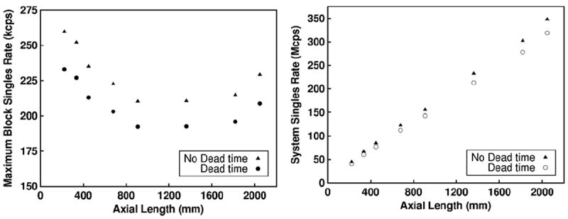
Maximum block singles rate and total system singles rate at the optimal activity concentration where peak NECR occurs is plotted as a function of axial length for all scanners with 20 mm thick detector blocks. The singles rate was characterized with dead time and no dead time to show the singles count loss rate.

Figure 8.

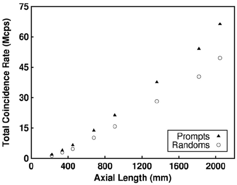
Total system coincidence rate at the optimal activity concentration where peak NECR occurs is plotted as a function of axial length for all scanners with 20 mm thick detector blocks.

4. Discussion

4.1. Siemens biograph mCT validation

Simulations that directly model the pulse processing and coincidence generation methods implemented in actual scanners are not common in the literature. Wear et al (1998) provides a rare example, but modeling individual components of a scanner is generally difficult because of limited information from manufacturers about their designs, or incomplete physical characterization of phenomena such as optical transport in scintillators. For the most part, existing validated simulation models use analytical dead time models based on fitting experimental data from the scanner (Schmidtlien et al 2006, Michel et al 2006), use simplified coincidence processing algorithms (Schmidtlien et al 2006), or assume values for physical parameters that give reasonable agreement to experimental results (Jan et al 2005, Gonias et al 2007). Simulation data have also been scaled to offset sensitivity mismatches to achieve close agreement with experimental results (Jan et al 2005, Michel et al 2006, Gonias et al 2007). The risk with these approaches is that the methods used to develop and validate the simulation models may not scale with confidence beyond the exact phantom and scanner configuration used in the validation, and may result in larger errors when used for performance prediction. Alternatively, simpler models that are more generic have been used, but much larger errors are accepted from the outset (Badawi et al 2000, 2001, MacDonald et al 2008, 2011).

The validation simulation presented here closely follows the actual scanner implementation, with only two parameters (LSO background count-rate and the estimated density of the carbon fiber bed) obtained from the scanner to be modeled. Using this approach we have obtained close agreement with experimental results without the necessity of fitting or the use of sensitivity factors that do not have a well-described physical explanation. We therefore can be reasonably confident that the modeled components provide a scalable simulation environment that can be applied to different phantoms and scanner geometries. In particular, we believe that the likely performance for scanner geometries that represent an incremental change to the existing devices (for example, the addition of approximately 10–20 cm to the AFOV) are reasonably accurately predicted.

However, there remains a potential difficulty for the largest AFOV scanners modeled–they are far beyond anything that currently exists, and scale-up to these configurations is likely to involve engineering trade-offs that are currently unknown. Certainly some caution against over-interpretation of the accuracy of the results presented for these scanners is warranted. An argument may be made that the substantial amount of work involved in creating such a complex simulation model is only of moderate value in these cases, since future large AFOV scanners are likely to have different electronics and/or detectors and therefore different performance envelopes. For initial exploration of such a parameter space, it may be that simpler models with larger errors are just as effective in drawing a general picture of expected performance and design requirements. However, accurate modeling is required if accurate performance prediction for a specific scanner design is desired.

4.2. Scintillator volume optimization study

For a given volume of scintillator, the scanner configuration based on the axial length and detector thickness can be optimized to obtain the maximum count-rate performance. However, the extension of the AFOV requires more detector modules and PMTs, which increases the overall cost of the system. As an example, the optimal AFOV and detector thickness for a scanner with 10 l of scintillator material is approximately 44 cm and 10 mm respectively. Current commercial scanners such as the Siemens Biograph mCT are typically configured with an AFOV of 22 cm and 20 mm thick detectors with 10 l of scintillator volume.

The optimal configuration is not only a balance of sensitivity losses due to thinning detectors and sensitivity gains from longer AFOV, but also the phantom axial length relative to the scanner AFOV. As the AFOV of the scanner increases, the number of randoms due to singles outside the field of view decreases and the number of trues acquired also increases, which increases overall count-rate performance and the optimal activity concentration. This effect allows a relatively larger optimal AFOV to reach maximum NECR performance for a given scintillator volume.

For scanners with constant detector thickness and variable axial length, the peak NECR performance increases by a factor greater than the proportional increase in scintillator volume, which suggests that there is never a situation in which the introduction of septa can improve NECR, even when the axial acceptance angle is limited. This is broadly consistent with the results described by MacDonald et al (2011) for scanners with 30 cm AFOV.

Several factors were not accounted for in the optimization study. First, TOF was not modeled in the simulations. The overall image SNR with TOF increases by a multiplicative factor that is proportional to square root of the distance through the object over the time resolution (Conti 2009). The addition of TOF information may also shift the maximum accepted ring difference and activity concentration to a greater value for a given scanner configuration. Furthermore, thinner detectors may have slightly better timing resolution properties (Moses et al 1998), which may offset detection sensitivity losses.

Second, the use of NECR as an objective function has limitations. For example, long AFOV scanners with thick detectors achieve greater count-rate performance, but there is a spatial resolution penalty due to DOI blurring in the axial direction for large acceptance angles that is not captured by NECR. Furthermore, the correlation between NEC and image SNR for the center voxel was derived assuming a 2D PET system with symmetric lines of response (LOR) passing through a uniform cylinder (Strother et al 1990). While correlation between NEC and image SNR has been experimentally demonstrated for 3D PET, such work has, to date, been performed only on systems with conventional geometries (Dahlbom et al 2005). Direct correlation between NEC and image SNR has not been validated for longer scanners modeled in this paper.

NECR also fails to capture variations in performance with respect to the position in the field of view. The performance in the central third of the scanner will likely be greater than suggested by NECR, and conversely the performance at the axial extremes will be worse. The average height of males in the US is 176 cm (McDowell et al 2008). If a typical male is placed centrally in a 2 m scanner, the sensitivity for the brain would not be better than obtainable with a 30 cm AFOV scanner. However, if the brain is of specific interest, the patient may be positioned asymmetrically in the scanner to obtain improved sensitivity.

The pre-whitened observer SNR is an alternative objective function that offers the potential to capture the effects of count-rate, TOF, and spatial resolution on image quality as a function of position in the field of view (Qi et al 2002). We hope to investigate design trade-offs in future studies using this metric.

4.2.1. Coincidence processing

Coincidence processing with a variable time window as a function of ring difference moderately increases the count-rate performance, especially for long AFOV scanner configurations. For the longest AFOV scanner configuration, the count-rate performance increases by approximately 10% compared to using a static coincidence time window based on the longest ring difference. The gain in NECR performance is mainly due to minimizing randoms from long LOR, which allows the system to operate with a larger maximum accepted ring difference.

4.3. Long axial field of view scanners

The results from the simulations show a significant increase in the peak NECR performance of approximately 25 times relative to the Siemens mCT Biograph scanner for a 2 m long AFOV scanner with 20 mm thick detectors (31 times higher NECR was observed for a fixed ~5 mCi injected dose). Further gains may be possible by implementation of TOF, which would be expected to have greater benefits in a long AFOV scanner compared to current conventional designs. A highly sensitive long AFOV scanner could then also support finer crystal segmentation, although it may become necessary to add some level of DOI capability as well. These significant gains may shift the current paradigm of human PET imaging, as it overcomes many current limitations. A high sensitivity and high spatial resolution PET system would enable imaging studies not feasible today, for example whole-body dynamic PET, stem cell trafficking, and low dose longitudinal studies in pediatric and normal populations.

4.3.1. Cost concerns

On the surface, a 2 m long AFOV PET scanner is potentially cost prohibitive, which would prevent commercial development and wide-spread deployment. However, it is estimated that a 2 m AFOV PET scanner would cost approximately $7–8M at market, which is comparable to a commercial 7 T magnetic resonance imaging (MRI) scanner (Gagnon 2012). Given that image SNR scales linearly with field strength in MRI (Schick 2005), and if we assume that in PET the image SNR scales with the square-root of NEC, then the results reported in this paper suggest that benefits of moving from a conventional PET geometry to a 2 m AFOV design would be at least as great as the benefits of increasing field strength from 1.5 to 7 T (probably greater in the central third of the scanner and certainly greater at low activities). Furthermore, the geometry lends itself to whole-body applications that are not possible with current PET scanners. Thus the production of a 2 m AFOV PET scanner may not be as impractical as might be imagined at first glance.

4.3.2. Detector design

Building a 2 m long AFOV scanner is possible with currently available detector technology and system electronics. For long AFOV scanners with thick scintillators, the detector readout may require both DOI encoding and TOF capabilities to maximize image quality. Currently, block detectors using single channel PMTs are capable of achieving TOF resolution of approximately 500 ps, but may only be capable of having fairly coarse DOI capabilities with two layers of crystal elements (Barrtzakos et al 1991). This may be sufficient for whole-body imaging applications.

Detector dead-time does not significantly paralyze the system at peak NECR for long AFOV scanners. Although the simulations use block detectors, quadrant sharing or zone-triggering based detectors may possibly be utilized as a cost effective method to reduce the number of channels required for detector read out. However, the performance of different specific detector designs can vary substantially for a variety of reasons, such as light sharing between adjacent crystals, light collection of photo detectors, and the design of front-end electronics to read-out events. Such detectors would need to be tested at the flux rates predicted in this study prior to use in a long AFOV scanner. At the same time, slower scintillators without background radioactivity, such as BGO, might also be viable candidates if the detector design is implemented with care, since peak NECR is obtained at injected doses that are substantially higher than those typically used in clinical protocols. Low activity studies, such as stem cell trafficking, may benefit from not having background that ¹⁷⁶Lu based scintillators possess. We note that bolus injections for quantitative imaging are not modeled in this study, which could produce very high local flux rates.

4.3.3. System electronics design

The simulations for the 2 m long AFOV scanner provide a guide for the electronic bandwidth requirements to process qualified single and coincidence events. At peak NECR, each block detector needs to process approximately 250 kcps, while the total qualified singles rate for the system is approximately 350 Mcps. The total prompt coincidence rate is approximately 70 Mcps using the optimal ring difference. The OpenPET electronics that is currently being developed for the community has the potential to provide the necessary bandwidth for each aspect of the system (Moses et al 2010).

5. Conclusion

In our work, we developed simulation models based on individual components used in the Siemens Biograph mCT. The combined simulation models were validated against experimental data with less than 8% error using the NEMA NU-2 2007 count-rate test. Using the validated simulation models, we investigated the optimization of scintillator volume to maximize count-rate performance in various scanner configurations. For a given scintillator volume, the optimization of AFOV and detector thickness results in modest count-rate performance gains of up to 16% relative to the shortest AFOV scanner. However, the relative gains from optimization diminishes as the scintillator volume increases.

We also obtained count-rate performance results for long AFOV scanners. To minimize the effect of randoms, we implemented a variable coincidence time window algorithm, which resulted in increasing count-rate performance approximately 10% compared to using a static coincidence time window based on the largest ring difference. Overall, the longest AFOV of approximately 2 m with 20 mm thick detectors resulted in performance gains of 25–31 times relative to the current Siemens Biograph mCT scanner configuration.

References

- Badawi RD, Adam LE, Zimmerman RE. A simulation-based assessment of the revised NEMA NU-2 70 cm long test phantom for PET. IEEE Nuclear Science Symp Conf Record. 2001:1466–70. [Google Scholar]
- Badawi RD, Kohlmyer SG, Harrison RL, Vannoy SD, Lewellen TK. The effect of camera geometry on singles flux, scatter fraction, and trues and randoms sensitivity of cylindrical 3D PET–a simulation study. IEEE Trans Nucl Sci. 2000;47:1228–32. [Google Scholar]
- Barrtzakos P, Thompson CJ. A depth-encoded PET detector. IEEE Trans Nucl Sci. 1991;38:732–8. [Google Scholar]
- Bettinardi V, Danna M, Savi A, Lecchi M, Castiglioni I, Gilardi MC, Bammer H, Lucignani G, Fazio F. Performance evaluation of the new whole-body PET/CT scanner: discovery ST. Eur J Nucl Med Mol Imaging. 2004;31:867–81. doi: 10.1007/s00259-003-1444-2. [DOI] [PubMed] [Google Scholar]
- Binkly DM, Puckett BS, Swann BK, Rochelle JA, Musrock MS, Casey ME. A 10-mc/s, 0.5-μm CMOS constant-fraction discriminator having built-in pulse tail cancellation. IEEE Nucl Trans Nucl Sci. 2002;49:1130–40. [Google Scholar]
- Casey ME. Siemens medical solutions molecular imaging private communication 2011 [Google Scholar]
- Cherry SR. The 2006 Henry N Wagner lecture: of mice and men (and positrons)–advances in PET imaging technology. J Nucl Med. 2006;47:1735–45. [PubMed] [Google Scholar]
- Conti M. Tailoring PET time coincidence window using CT morphological information. IEEE Trans Nucl Sci. 2007;54:1599–605. [Google Scholar]
- Conti M. State of the art and challenges of time-of-flight PET. Phys Medica. 2009;25:1–11. doi: 10.1016/j.ejmp.2008.10.001. [DOI] [PubMed] [Google Scholar]
- Conti M, Rothfuss H. Time resolution for scattered and unscattered coincidences in a TOF PET scanner. IEEE Trans Nucl Sci. 2010;57:2538–44. [Google Scholar]
- Conti M, et al. Performance of a high sensitivity PET scanner based on LSO panel detectors. IEEE Trans Nucl Sci. 2006;53:1136–42. [Google Scholar]
- Cook GJR, Lodge MA, Marsden PK, Dynes A, Fogelman I. Non-invasive assessment of skeletal kinetics using fluorine-18 positron emission tomography: evaluation of image and population-derived arterial input functions. Eur J Nucl Med. 1999;26:1424–9. doi: 10.1007/s002590050474. [DOI] [PubMed] [Google Scholar]
- Couceiro M, Ferreira NC, Fonte P. Sensitivity assessment of wide axial field of view PET system via Monte Carlo simulations of NEMA-like measurements. Nucl Instrum Methods Phys Res A. 2007;580:485–8. [Google Scholar]
- Dahlbom M, Schiepers C, Czernin J. Comparison of noise equivalent count rates and image noise. IEEE Trans Nucl Sci. 2005;52:1386–90. [Google Scholar]
- De Geus-Oei LF, Visser EP, Krabbe PFM, van Hoorn BA, Koenders EB, Willemsen AT, Prium J, Corsten FHM, Oyen WJG. Comparison of image-derived and arterial input functions for estimating the rate of glucose metabolism in therapy-monitoring 18F-FDG PET studies. J Nucl Med. 2006;47:945–9. [PubMed] [Google Scholar]
- Eriksson L, Townsend D, Conti M, Eriksson M, Rothfuss H, Schmand M, Casey ME, Bendriem B. An investigation of sensitivity limits in PET scanners. Nucl Instrum Methods Phys Res A. 2007;580:836–42. [Google Scholar]
- Eriksson L, Townsend DW, Conti M, Melcher CL, Eriksson M, Jakoby BW, Rothfuss H, Casey ME, Bendriem B. Potentials of large axial field of view positron camera systems. IEEE Nuclear Science Symp Conf Record. 2008:1632–6. [Google Scholar]
- Fakhri GE, Surti S, Trott CM, Scheuermann J, Karp JS. Improvement in lesion detection with whole-body oncologic time-of-flight PET. J Nucl Med. 2011;52:347–53. doi: 10.2967/jnumed.110.080382. [DOI] [PMC free article] [PubMed] [Google Scholar]
- Ferrero A, Poon JK, Chaudhari AJ, MacDonald LR, Badawi RD. Effect of object size on scatter fraction estimation methods for PET–a computer simulation study. IEEE Nucl Trans Nucl Sci. 2011;58:82–6. [Google Scholar]
- Gagnon D. Toshiba Medical Research Institute USA private communication 2012 [Google Scholar]
- Gonias P, et al. Validation of a GATE model for the simulation of the Siemens Biograph 6 PET scanner. Nucl Instrum Methods Phys Res A. 2007;571:263–6. [Google Scholar]
- Jakoby BW, Bercier Y, Conti M, Casey ME, Bendriem B, Townsend BW. Physical and clinical performance of the mCT time-of-flight PET/CT scanner. Phys Med Biol. 2011;56:2375–89. doi: 10.1088/0031-9155/56/8/004. [DOI] [PubMed] [Google Scholar]
- Jan S, Comtat C, Strul D, Santin G, Trébossen R. Monte Carlo simulation for the ECAT EXACT HR +system using GATE. IEEE Trans Nucl Sci. 2005;52:627–33. [Google Scholar]
- Jan S, et al. GATE: a simulation toolkit for PET and SPECT. Phys Med Biol. 2004;49:4543–61. doi: 10.1088/0031-9155/49/19/007. [DOI] [PMC free article] [PubMed] [Google Scholar]
- Kapusta M, Szuprycynski P, Melcher CL, Moszyński M, Balcerzyk M, Carey A, Aczarnacki W, Spurrier MA, Syntfeld A. Non-proportionality and thermoluminescence of LSO:Ce. IEEE Trans Nucl Sci. 2005;52:1098–104. [Google Scholar]
- Karakatsanis NA, Lodge MA, Zhou Y, Mhlanga J, Chaudhry M, Tahari AK, Segars WP, Wahl RL, Rahmim A. Dynamic multi-bed FDG PET imaging: feasibility and optimization. IEEE Nuclear Science Symp Conf Record. 2011:3863–70. [Google Scholar]
- Karp JS, Surti S, Daube-Witherspoon ME, Muehllehner G. Benefit of time-of-flight in PET: experimental and clinical results. J Nucl Med. 2008;49:462–70. doi: 10.2967/jnumed.107.044834. [DOI] [PMC free article] [PubMed] [Google Scholar]
- Lortie M, Beanlands RSB, Yoshinaga K, Klein R, DaSilva JN, deKemp RA. Quantification of myocardial blood flow with 82Rb dynamic PET imaging. Eur J Nucl Med Mol Imaging. 2007;34:1765–74. doi: 10.1007/s00259-007-0478-2. [DOI] [PubMed] [Google Scholar]
- MacDonald LR, Harrison RL, Alessio AM, Hunder WCJ, Lewellen TK, Kinahan PE. Effective count rates for PET scanners with reduced and extended axial field of view. Phys Med Biol. 2011;56:3629–43. doi: 10.1088/0031-9155/56/12/011. [DOI] [PMC free article] [PubMed] [Google Scholar]
- MacDonald LR, Schmitz RE, Alessio AM, Wollenweber SD, Stearns CW, Ganin A, Harrison RL, Lewellen TK, Kinahan PE. Measured count-rate performance of the Discovery STE PET/CT scanner in 2D, 3D, and partial collimation acquisition modes. Phys Med Biol. 2008;53:3723–38. doi: 10.1088/0031-9155/53/14/002. [DOI] [PMC free article] [PubMed] [Google Scholar]
- McDowell MA, Fryar CD, Ogden CL, Flegal KM. Anthropometric reference data for children and adults: United States, 2003–2006 1–45. National Helath Statistics Reports. 2008;10 [PubMed] [Google Scholar]
- Michel C, Eriksson L, Rothfuss H, Bendriem B. Influence of crystal material on the performance of the HiRez 3D PET scanner: a Monte Carlo study. IEEE Nuclear Science Symp Conf Record. 2006:2528–31. [Google Scholar]
- Moses WW, Buckley S, Vu C, Peng Q, Pavlov N, Choong W, Wu J, Jackson C. OpenPET: a flexible electronics system for radiotracer imaging. IEEE Trans Nucl Sci. 2010;57:2532–7. doi: 10.1109/NSSMIC.2009.5401797. [DOI] [PMC free article] [PubMed] [Google Scholar]
- Moses WW, Derenzo SE. Prospects for time-of-flight PET using LSO scintillator. IEEE Trans Nucl Sci. 1999;46:474–80. [Google Scholar]
- Mourik J, Lubberink M, Schuitemaker A, Tolboom N, van Berckel BNM, Lammertsma AA, Boellaard R. Image-derived input functions for PET brain studies. Eur J Nucl Med Mol Imaging. 2009;36:463–71. doi: 10.1007/s00259-008-0986-8. [DOI] [PubMed] [Google Scholar]
- Qi J, Kuo C, Huesman RH, Klein GJ, Moses WW, Reutter BW. Comparison of rectangular and dual-planar positron emission mammography scanners. IEEE Trans Nucl Sci. 2002;49:2089–96. [Google Scholar]
- Schick F. Whole-body MRI at high field: technical limits and clinical potential. Eur Radiol. 2005;15:946–59. doi: 10.1007/s00330-005-2678-0. [DOI] [PubMed] [Google Scholar]
- Schmidtlein CR. Validation of GATE Monte Carlo simulations of the GE advance/discovery LS PET scanners. Med Phys. 2006;33:198–208. doi: 10.1118/1.2089447. [DOI] [PubMed] [Google Scholar]
- Strother SC, Casey ME, Hoffman EJ. Measuring PET scanner sensitivity: relating countrates to image signal-to-noise ratios using noise equivalent counts. IEEE Trans Nucl Sci. 1990;37:783–8. [Google Scholar]
- Surti S, Karp JS. Imaging characteristics of a three-dimensional GSO whole-body PET camera. J Nucl Med. 2004;45:1040–9. [PubMed] [Google Scholar]
- Surti S, Lee E, Werner ME, Karp JS. Imaging study of a clinical PET scanner design using an optimal crystal thickness and scanner axial FOV. IEEE Nuclear Science Symp Conf Record. 2011:3390–4. [Google Scholar]
- Watanabe M, et al. A high-throughput whole-body PET scanner using flat panel PS-PMTs. IEEE Trans Nucl Sci. 2004;51:796–800. [Google Scholar]
- Wear JA, Karp JS, Freifelder R, Mankoff DA, Muehllehner G. A model of the high count rate performance of NaI(Tl)-based PET detectors. IEEE Trans Nucl Sci. 1998;45:1231–7. [Google Scholar]
- Wollenweber SD, Phillips KR, Stearns CW. Calculation of noise-equivalent image quality. IEEE Nuclear Science Symp Conf Record. 2003;4:2822–5. [Google Scholar]
- Wong WH, Zhang Y, Liu S, Li H, Baghaei H, Ramirez R, Liu J. The initial design and feasibility study of an affordable high-resolution 100-cm long PET. IEEE Nuclear Science Symp Conf Record. 2007;6:4117–22. [Google Scholar]
- Zhang S, Wu J. Comparison of imaging techniques for tracking cardiac stem cell therapy. J Nucl Med. 2007;48:1916–9. doi: 10.2967/jnumed.107.043299. [DOI] [PMC free article] [PubMed] [Google Scholar]