Quantifying the effect of temporal resolution on time-varying networks

Abstract

Time-varying networks describe a wide array of systems whose constituents and interactions evolve over time. They are defined by an ordered stream of interactions between nodes, yet they are often represented in terms of a sequence of static networks, each aggregating all edges and nodes present in a time interval of size Δt. In this work we quantify the impact of an arbitrary Δt on the description of a dynamical process taking place upon a time-varying network. We focus on the elementary random walk, and put forth a simple mathematical framework that well describes the behavior observed on real datasets. The analytical description of the bias introduced by time integrating techniques represents a step forward in the correct characterization of dynamical processes on time-varying graphs.

Time-varying networks are ubiquitous. Examples are found in the social, cognitive, technological and ecological domains as well as in many others¹. The temporal nature of such systems has a deep influence on dynamical processes occurring on top of them²,³,⁴,⁵,⁶,⁷,⁸,⁹,¹⁰,¹¹,¹²,¹³,¹⁴,¹⁵,¹⁶,¹⁷,¹⁸,¹⁹,²⁰,²¹. Indeed, the spreading of sexual transmitted diseases, the diffusion of topics over social networks, and the propagation of ideas in scientific environments are affected by duration, sequence, and concurrency of contacts²,⁴,¹⁷,¹⁸,¹⁹,²²,²³. In all these cases the timescale characterizing the evolution of the network is comparable with the timescale ruling the unfolding of the process, and they cannot be decoupled. However, empirical datasets are often reduced to a series of static networks by introducing a time-integrating window, Δt¹,²⁴,²⁵,²⁶,²⁷. This is the case, for instance, of face-to-face interaction networks²⁸, for which the fine-grained temporal resolution of (e.g.) phone call networks is not available, or of infants' semantic networks²⁹, whose evolution can be studied only through the analysis of few snapshots³⁰. In other instances, a time window is introduced to reduce the amount of stored information, or to simplify the application of mathematical frameworks developed for static or annealed systems. This is the case, for example, of online social networks where, although usually the original information has time resolutions down to the second, the available datasets are integrated over different windows of hours, days, months, or even years. Thus, the introduction of an integrating window is either intrinsic to the system under study or dictated by practical reasons.

In this work we address the impact of an arbitrary Δt on the description of a discrete dynamical process taking place upon a time-varying network. Despite recent results showing that the presence of any level of temporal aggregation may affect the correct characterization of dynamical processes evolving on top of such datasets²,³,⁴,⁵,⁶,⁷,⁸,⁹,¹⁰,¹¹,¹²,¹³,¹⁴,¹⁵,¹⁶,¹⁷,¹⁸,¹⁹,²⁰,²¹, an analytical formalization, characterization, and understanding of these effects for a general Δt is still missing.

In particular, we focus on the prototypical random walk process evolving on time-varying networks integrated over a general time window Δt. First, we clarify the relevance of the integrating window issue by studying the behavior of random walk processes on real time-varying networks as a function of Δt. Then, we introduce a mathematical framework that well describes the observed behavior on synthetic activity driven networks¹⁷ as well as on two different real datasets.

Results

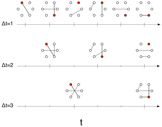
We aim to understand how Δt affects the behavior of dynamical processes taking place on time-varying networks. To this end, we consider the fundamental random walk (RW) process on two different real time-varying networks in which the links have been integrated over different integrating windows Δt (see Fig. 1). Typically, the RW asymptotic occupation probability ρ (see Methods for the formal definition) is computed grouping the nodes according to their the degree k³¹,³²,³³. The quantity ρ_k is then defined as the average asymptotic occupation probability of a node in the degree class k³¹,³²,³³. However, in time-varying networks the degree of a node is not univocally defined and, more importantly, is a function of Δt. For example, the degree might be the number of connections integrated over the time window, or the average number of connections across the T/Δt static frames (where T is the total time span of the data). Thus, the same node could contribute to different degree classes depending on the value of Δt. We, therefore, focus on a different node measure that has been shown to be mostly invariant to Δt, namely the activity rate a of a node¹⁷. The activity rate a is defined as the average rate at which each node interacts with others during the observation period [0, T], and can be interpreted as the intrinsic attitude of each node to engage in interactions with other nodes. We aim to calculate the occupation probability as a function of a.

Figure 1. Example of time integration on time-varying networks.

The random walker is located on the colored node, and can travel on the links depicted as continuous line, while Δt defines the integration window. Dashed lines represent links that are present in the system, but are out of reach for the walker.

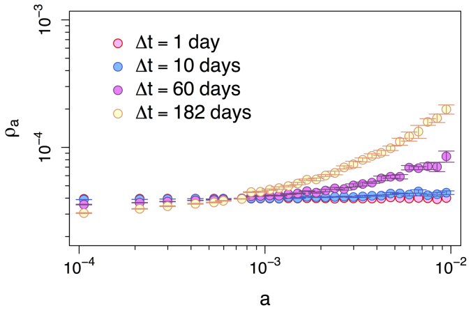
In our simulations we consider two real time-varying networks, and investigate the RW occupation probability function of activity rate a and the integrating window Δt: ρ_a(Δt). The first dataset is the co-authorship network of the Physical Review Letters (PRL) journal from 1980 to 2006³⁴. The second dataset is the Yahoo! music dataset with ~4.6 × 10⁵ songs rated by ~2 × 10⁴ Yahoo! users over six months³⁵. We run the RW process over these two time-varying networks for different values of Δt, and record the occupation probability over multiple runs (see SI for details). Fig. 2 shows the empirical values of ρ_a(Δt) (solid points) observed in the PRL dataset for four distinct values of Δt = {1, 10, 60, 182} days. Error bars represent the the standard deviation obtained from distinct simulation runs starting at times t₀ ∈ {0, 1, …, Δt − 1} from the beginning of the dataset.

Figure 2. Occupation probability ρ_a of a RW at the end of the simulation as a function of node activity.

The points are the values of ρ_a of a RW over the Physics Review Letters time-varying co-authorship network from 1980 to 2006 for different integrating windows Δt ∈ {1, 10, 60, 182} days. The error bars are evaluated starting the process at different days from the beginning of the dataset.

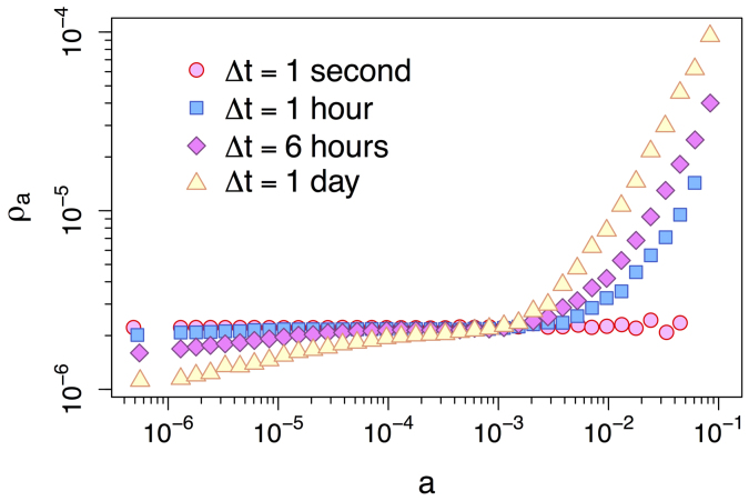
The effect of Δt is dramatic. Over large values of Δt the RW behaves roughly as could be expected. The share of random walkers increases with the node activity, i.e., highly active nodes are collect more walkers at the end of the simulation than nodes with low activity. However, as Δt decreases, more active nodes lose their power to attract walkers and the occupation probability becomes more uniform. A similar scenario is observed over the Yahoo! dataset over four values of Δt, namely one second, one hour, six hours, and one day (points in Fig. 3). In the next section we will see that the reason for this behavior rests solely in the probability that the RW sees no edges when it decides to move, which turns out to be a function of three factors: Δt, the activity of node the walker resides, and the average node activity in the system.

Figure 3. Occupation probability ρ_a of a RW at the end of the simulation as a function of node activity.

Points represent the ρ_a values of a RW over the time-varying graph of Yahoo! song ratings for different integrating windows Δt of one second, one hour, six hours, and one day. The standard deviations are too small to be shown in the plots.

Mathematical formulation

Let us consider a random walker diffusing at discrete time steps Δt over a time-varying network characterized by N nodes. Starting at node V (t) at step t, the walker takes step t + 1 at time (t + 1) Δt diffusing over a network G_t(Δt), where G_t(Δt) is the result of the union of all the edges generated in the interval [tΔt, (t + 1) Δt). We focus on the general case of an arbitrary time aggregation window Δt > 0.

We consider a simple class of time-varying networks called activity driven networks¹⁷. The crucial ingredients of these models are: dF(a), the fraction of nodes with activity rate a, and m, the number of edges that are simultaneously created by a node (see Methods for further details). The activity rate determines the probability per unit time for a node to establish (m, simultaneously) edges to other nodes in the system. The value of parameter m is dictated by the specific system under consideration. The case m > 1 is appropriate to describe one-to-many interactions, found for example in such systems as Twitter and blog networks³⁶,³⁷. On the other hand, m = 1 describes two-party (dyadic) communications that are characteristic of phone-call and text-message networks³⁸,³⁹. At each step t = 0, 1, … an unweighted network G_t(Δt) is generated as follows:

1. G_t(Δt) starts with N disconnected nodes;

2. The the number of times a node with activity a is active during interval Δt, K_Δt,a, is Poisson distributed Node generates mK_Δt,a undirected edges connected to mK_Δt,a randomly selected nodes (without replacement or self-loops). Inactive nodes in this observed period of Δt may receive connections from other active vertices;

3. At time (t + 1)Δt the process starts over from step a) to generate network G_t+1(Δt).

Although activity driven networks are Markovian (memoryless) and lack of some properties observed in real temporal systems, they can be considered as the simplest yet nontrivial framework to study the concurrence of changes in connectivity pattern of the network and dynamical processes unfolding on their structure¹⁷,¹⁸.

To describe the RW behavior, we need to evaluate the transition probability that a walker starting at a node with activity a′ moves to a node with activity a at the next Δt time step, Q_a|a′(Δt). Without loss of generality in what follows we focus on the case m = 1. Detailed results for the m > 1 one-to-many interactions are discussed in the Supplementary Information. At step t + 1 the neighbors of V (t) can be classified into two types:

1. Passive destinations, are neighbors of V (t) connected by edges created due to the activity of V (t) itself. They are randomly selected from the graph and thus their activity is distributed according to dF(a). We define K_Δt,A(t) to be the number of such passive destinations, where A(t) is the activity rate of node V (t).

2. Active destinations, are neighbors of V (t) connected to V (t) by edges created due to their own activity. Thus, their activity is distributed as adF(a)/〈a〉, where 〈a〉 is the average activity rate in the system. We define define H_Δt as the number of such active destinations.

The word destinations highlights the fact that the walker moves from V (t) to one of these K_Δt,a′ + H_Δt neighbors of V (t). For sufficiently large N, H_Δt and K_Δt,a′ are both Poisson distributed with average 〈a〉Δt and a′Δt, respectively. If V (t) has at least one edge, the walker follows the edge of a passive destination with probability K_Δt,a′/(K_Δt,a′ + H_Δt), while it moves towards an active destination with probability H_Δt/(K_Δt,a′+ H_Δt). Unconditioning the latter expressions with respect to the values of K_Δt,a′ and H_Δt we obtain

where δ(x) is the Dirac delta function. While we refer the reader to the SI for the detailed derivation, each term in eq. (1) has a simple interpretation. The two terms inside the double sum represent, respectively, the probability that the walker moves to a passive destination that has activity a and the probability that the walker moves to an active destination that has activity a. The terms multiplying the two terms inside the double summation are related to the probability that K_Δt,a′ = k and H_Δt = h. The δ(a − a′) term considers the probability that the node has no edges after Δt and thus the walker must remain at V (t).

Thankfully, eq. (1) can be simplified (see SI) yielding

where ζ_a′,Δt = e^{−(a′+〈a〉)Δt} is the probability that no edge is created at a node with activity a′ during interval Δt. Note that in eq. (2) the parameter Δt only affects the probability that no edge is created until the next time step.

To find the RW stationary distribution we first note that the RW on the time-varying network is stationary and ergodic (see SI). Thus, the RW occupation probability ρ_a, defined as the probability of finding the walker in a given node of activity a, exists and is unique⁴⁰. The value of ρ_a is the fixed point solution of the following Chapman-Kolmorogov set of equations⁴¹

where Ω is the set of all activity rates in the system. The solution to eq. (3) can be obtained numerically. Interestingly, we can extend eq. (3) to consider lazy random walks where the walker moves with probability p ∈ (0, 1] or does not move with probability 1 − p. For the lazy walker we just need to replace Q_a|a′(Δt) in eq. (3) with Q_a|a′(Δt)p + δ(a′ − a)(1 − p). A simple algebraic manipulation shows that ρ_a does not change with p. Hence, the steady state of the lazy walker for any p ∈ (0, 1) is the same as the walker that moves with probability p = 1.

We also find that closed-form solutions of eq. (3) exist in the limits of and . In the case, links are integrated over a large time window and the time-varying network can be considered static. Recall that ζ_a,Δt = e^{(a+〈a〉)Δt}. For the value of ζ_a,Δt ≈ 0, ∀a ∈ Ω, and thus the second term of eq. (2) is close to zero. In this scenario Q_a|a′(Δt) = C(a + 〈a〉)dF(a), where C = 1/2〈a〉 yielding the fixed point solution of eq. (3)

The asymptotic occupation probability of a given node of class a is simply proportional to its activity. Since in the regime of large Δt the degree of a node v, k_v, is proportional to its activity, a_v, eq. (4) yields . Thus, for sufficiently large Δt, we recover the well-known behavior of static networks, where the occupation probability of a node is proportional to its degree³¹. Furthermore, in the SI we show that eqs. (2), (3), and (4) hold for weighted aggregation procedures where integrated edges have weights proportional to how often they appeared during an interval Δt.

In the regime of very short aggregating windows we have lim_Δt→0 ζ_a,Δt → 1, ∀a ∈ Ω. Thus, the first term of eq. (2) is zero yielding Q_a|a′(Δt) = dF(a) and the trivial fixed point solution of eq. (3)

Thus, the walker is equally likely to be found at any node regardless of its activity rate. In fact, when Δt is small the probability a node has more than one edge is close to zero. Consequently, highly active nodes lose and gain walkers at the same rate, giving rise to homogeneous occupation probabilities in eq. (5). Interestingly, in previous work on general time-varying network processes we show that the result in eq. (5) holds even when aggregated snapshots have arbitrary strong spatio-temporal correlations⁴⁰.

Numerical validation on synthetic networks

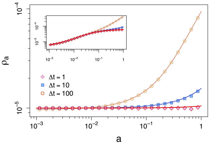
We validated our analytical results through extensive numerical simulations. We considered networks with N = 10⁵ nodes and a power-law activity distribution dF(a) ∝ a^−γ (as observed in many real networks¹⁷), restricted to the interval Ω = [10⁻³, 1] to avoid divergencies in the limit . As shown in Fig. 4, the exact solution reproduces the simulations accurately for the entire spectrum of integrating windows Δt (case m = 1 in main panel). Interestingly, as Δt grows, the occupation probability increases sharply in high-activity vertices while slightly decreasing at low activity nodes. Moreover, as Δt increases ρ_a ∝ a as predicted by eq. (4), while as Δt gets smaller, ρ_a = 1/N, as predicted by eq. (5). The equations describe correctly also the behavior observed for one-to-many simultaneous connections m, characterized by a smoother increase in ρ_a at high activity nodes (see m = 6 case in Fig. 4, inset). The SI contains more details on the formulation of the m > 1 case.

Figure 4. Occupation probability ρ_a of a RW over an activity-driven network with activity distribution dF(a) ∝ a⁻², a ∈ (10⁻³, 1), N = 10⁵, for different values of m.

Curves in the main plot concern the m = 1 case, where each node can only simultaneously connect to one node. In the inset, the case m = 6 is considered, where a node simultaneously connect to six other nodes. Solid curves represent the analytical prediction of eq. (3) integrated over Δt = 1, 10, 100 (diamonds, squares and circles) time windows. Note that in both panels as Δt gets larger ρ_a ≈ a. Averages performed over 10³ independent simulations.

Numerical validation on real-world networks

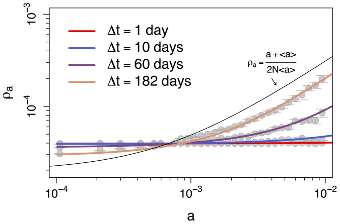
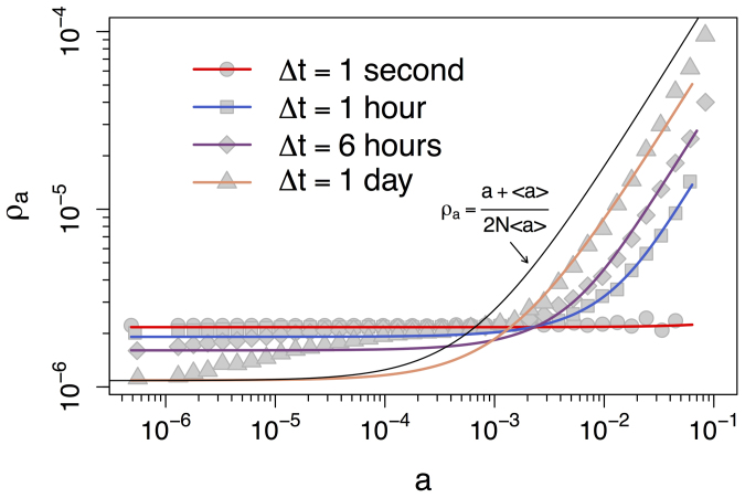
The analytical framework discussed above qualitatively reproduce also the behavior observed in real datasets. In Figs. 5 and 6 the solid lines show the numerical solution obtained by applying eq. (2) into eq. (3) (see SI), for the PRL and Yahoo! datasets, respectively. The gray points in Figs. 5 and 6 reproduce the simulation results already shown in Figs. 2 and 3, respectively. All numerical solutions use the same activity distribution dF(a), extracted from the time-varying graph of Δt = 1 day for the PRL dataset and Δt = 1 second for the Yahoo! dataset (dF(a) extracted from larger values of Δt provide similar results¹⁷, see SI for details).

Figure 5. Occupation probability ρ_a of a RW at the end of the simulation as a function of node activity.

The points are the values of ρ_a of a RW over the Physics Review Letters time-varying co-authorship network from 1980 to 2006 for different integrating windows Δt ∈ {1, 10, 60, 182} days. The solid curves show the respective numerical solutions of eq. (3) and the black curve shows eq. (4).

Figure 6. Occupation probability ρ_a of a RW at the end of the simulation as a function of node activity.

The points are the values of ρ_a of a RW over the time-varying graph of Yahoo! song ratings for different integrating windows Δt of one second, one hour, six hours, and one day. The solid curves show the respective numerical solutions of eq. (3) and the black curve shows eq. (4).

The theoretical results accurately describe real data, with some deviations for nodes in the intermediate activity range at Δt of one day. The RW occupation probability is uniform and independent of node activity for small Δt as predicted by eq. (5). As predicted by eq. (4), the RW occupation probability ρ_a approaches (a + 〈a〉)/(2N〈a〉) (black curve) as Δt increases, an effect particularly noticeable for high-activity nodes. It is also worth highlighting that the data matches well the theoretical equations for the case m = 1, suggesting a connection between the datasets and the fundamental mechanisms described in our model (for the similarity in behavior between m = 1 and projected networks such as the PRL co-authorship networks see SI).

Discussion

Our results clarify the effect of time aggregation procedures on the behavior of the RW, taken as the simplest instance of dynamical process, even when aggregation windows are “short”. We have quantified this effect in a rigorous mathematical framework that (i) allows us to recover the results concerning static networks in the limit of infinite aggregation windows, (ii) accurately describes the behavior observed in numerical simulations upon synthetic time-varying networks, and (iii) captures the phenomenology observed on real datasets. Overall, while for practical or technical reasons researchers are often forced, or simply tempted, to work with time aggregated representations of time-varying networks, our work suggests that caution should be used when drawing general conclusions about dynamical processes based upon time-aggregated networks. At the same time, moreover, our theoretical results may help to investigate possible distortions introduced by the aggregating windows of data collection methods.

The proposed framework considers inherently discrete processes, such as spreading phenomena in contact networks that are, also at the smallest time resolution possible, discrete. We leave the generalization to continuous processes for further work.

Methods

Occupation probability

The asymptotic occupation probability is the steady state probability of finding the walker in a node with activity a, which is guaranteed to exist and be unique if the time-varying network that is stationary, ergodic, and T-connected (see SI), such as in activity driven networks. A time-varying network is T-connected if there is a temporal path between any two nodes⁴⁰. In our simulations we consider the RW occupation probability ρ_a to be the probability of finding the walker in a node with activity a at the end of the simulation period [0, T], given the walker starts at a random node.

Activity-driven networks

Activity-driven network models are based on the activity patterns of nodes, that are used to explicitly model the evolution of the network structure over time¹⁷. It can be shown that the full dynamics of the network are encoded in the activity rate distribution, dF(a) and that the time-aggregated measurement of network connectivity yields a degree distribution that follows the same functional form as the distribution dF(a) in the limit of small k/Δt and k/N¹⁷. This is an important feature of the model, that is able to reproduce basic statistical properties found in many real networks giving a simple prescription to characterize explicitly dynamical connectivity patterns.

Datasets & simulation

In this study we considered two different empirical projections of bipartite time-varying networks. The collaborations in the journal Physical Review Letters (PRL) published by the American Physical Society³⁴, and the Yahoo! music dataset made available by Yahoo!³⁵.

PRL dataset

The bipartite network representation of this dataset has two type of nodes: authors and papers. An author is connected to all the papers she/he wrote in a integrating window Δt. We study the bipartite projection of the authors. In this representation each author of an article in PRL as a node. Undirected edges connect authors that collaborate in the same article. We focus just on small collaborations filtering out all the articles with more than 10 authors. We consider the period between 1958 and 2006. The datasets contains 80,554 authors and 66,892 articles. The smallest timescale available is one day.

Yahoo! music dataset

In this dataset the bipartite network has two type of nodes: users and songs. We study the bipartite projection over the songs. Each node is a song and two songs are connected if at least one user rated both in a time window Δt. The dataset contains 4.6 × 10⁵ songs rated by 199,719 users of Yahoo! users collected in the course of six months³⁵. User activity is recorded at a time resolution of seconds.

Simulation setup

We obtain the empirical walker occupation probability, ρ_a, as follows. Construct the transition probability matrix P_t associated to the RW on the t-th aggregated network G_t(Δt), t = 0, …, T/Δt, where T is the time of the last event in the dataset. The empirical RW occupation probability is obtained by multiplying the matrices and then left-multiplying the result by the vector (1/N, …, 1/N), which gives equal probability that for the walker to start at any node. We note in passing that similar results are obtained when the walker starts at a handful of high activity nodes.

Author Contributions

B.R., N.P. & A.B. designed research, B.R. & N.P. performed simulations, B.R., N.P. & A.B. analyzed the data, B.R. derived the analytical results. All authors wrote, reviewed and approved the manuscript.

Supplementary Material

Supplementary Information

Supplementary Information Quantifying the effect of temporal resolution on time-varying networks

References

- Holme P. & Saramäki J. Temporal networks. Phys. Rep. 519, 97 (2012). [Google Scholar]
- Morris M. Telling tails explain the discrepancy in sexual partner reports. Nature 365, 437 (1993). [DOI] [PubMed] [Google Scholar]
- Morris M. Concurrent partnerships and syphilis persistence: new thoughts on an old puzzle. Sexually transmitted diseases 28, 504–507 (2001). [DOI] [PubMed] [Google Scholar]
- Clauset A. & Eagle N. Persistence and periodicity in a dynamic proximity network. In: DI-MACS Workshop on Computational Methods for Dynamic Interaction Networks 1–5 (2007). [Google Scholar]
- Vespignani A. Modeling dynamical processes in complex socio-technical systems. Nature Physics 8, 32–30 (2012). [Google Scholar]
- Rocha L. E. C., Liljeros F. & Holme P. Simulated epidemics in an empirical spatiotemporal network of 50,185 sexual contacts. PLoS Comput Biol 7, e1001109 (2011). [DOI] [PMC free article] [PubMed] [Google Scholar]
- Isella L. et al. What's in a crowd? analysis of face-to-face behavioral networks. J. Theor. Biol 271, 166 (2011). [DOI] [PubMed] [Google Scholar]
- Stehlé J. et al. Simulation of an seir infectious disease model on the dynamic contact network of conference attendees. BMC Medicine 9 (2011). [DOI] [PMC free article] [PubMed] [Google Scholar]
- Karsai M. et al. Small but slow world: How network topology and burstiness slow down spreading. Phys. Rev. E 83, 025102 (2011). [DOI] [PubMed] [Google Scholar]
- Miritello G., Moro E. & Lara R. Dynamical strength of social ties in information spreading. Phys. Rev. E 83, 045102 (2011). [DOI] [PubMed] [Google Scholar]
- Kivela M. et al. Multiscale analysis of spreading in a large communication network. (2011). ArXiv:1112.4312v1.
- Fujiwara N., Kurths J. & Díaz-Guilera A. Synchronization in networks of mobile oscillators. Physical Review E 83, 025101 (2011). [DOI] [PubMed] [Google Scholar]
- Parshani R., Dickison M., Cohen R., Stanley H. E. & Havlin S. Dynamic networks and directed percolation. EPL (Europhysics Letters) 90, 38004 (2010). [Google Scholar]
- Bajardi P., Barrat A., Natale F., Savini L. & Colizza V. Dynamical patterns of cattle trade movements. PLoS ONE 6, e19869 (2011). [DOI] [PMC free article] [PubMed] [Google Scholar]
- Baronchelli A. & Díaz-Guilera A. Consensus in networks of mobile communicating agents. Phys. Rev. E 85, 016113 (2012). [DOI] [PubMed] [Google Scholar]
- Starnini M., Baronchelli A., Barrat A. & Pastor-Satorras R. Random walks on temporal networks. Phys. Rev. E 85, 056115 (2012). [DOI] [PubMed] [Google Scholar]
- Perra N., Gonçalves B., Pastor-Satorras R. & Vespignani A. Time scales and dynamical processes in activity driven networks. Sci. Rep. 2, 469 (2012). [DOI] [PMC free article] [PubMed] [Google Scholar]
- Perra N. et al. Random walks and search in time varying networks. Phys. Rev. Lett. 109, 238701 (2012). [DOI] [PubMed] [Google Scholar]
- Hoffmann T., Porter M. & Lambiotte R. Generalized master equations for non-poisson dynamics on networks. Physical Review E 86, 046102 (2012). [DOI] [PubMed] [Google Scholar]
- Krings G., Karsai M., Bernhardsson S., Blondel V. D. & Saramäki J. Effects of time window size and placement on the structure of an aggregated communication network. EPJ Data Science 1, 4 (2012). [Google Scholar]
- Holme P. Epidemiologically optimal static networks from temporal network data. (2013). [DOI] [PMC free article] [PubMed]
- Butts C. Relational event framework for social action. Sociological Methodology 38, 155–200 (2008). [Google Scholar]
- Toroczkai Z. & Guclu H. Proximity networks and epidemics. Physica A 378, 68–75 (2007). [Google Scholar]
- Maity S., Manoj T. & Mukherjee A. Opinion formation in time-varying social networks: The case of the naming game. Physical Review E 86, 036110 (2012). [DOI] [PubMed] [Google Scholar]
- Carley K. Dynamics network analysis. 133–145 (2003).
- Rosvall M. & Bergstrom C. T. Mapping change in large networks. PLoS ONE 5, e8694 (2010). [DOI] [PMC free article] [PubMed] [Google Scholar]
- Holme P. et al. On network bipartivity. e-print cond-mat/0302296 (2003). [Google Scholar]
- Cattuto C. et al. Dynamics of person-to-person interactions from distributed rfid sensor networks. PloS One 5, e11596 (2010). [DOI] [PMC free article] [PubMed] [Google Scholar]
- Baronchelli A., Ferrer-i Cancho R., Pastor-Satorras R., Chater N. & Christiansen M. H. Networks in cognitive science. Trends in cognitive sciences 17, 348–360 (2013). [DOI] [PubMed] [Google Scholar]
- Beckage N., Smith L. & Hills T. Small worlds and semantic network growth in typical and late talkers. PloS one 6, e19348 (2011). [DOI] [PMC free article] [PubMed] [Google Scholar]
- Noh J. & Rieger H. Random walks on complex networks. Phys. Rev. Lett. 92, 118701 (2004). [DOI] [PubMed] [Google Scholar]
- Newman M. Networks. An Introduction 157–159 (Oxford Univesity Press 2010). [Google Scholar]
- Barrat A., Barthélemy M. & Vespignani A. Dynamical Processes on Complex Networks, 160–163 (Cambridge Univesity Press, 2008). [Google Scholar]
- American Physical Society. Data sets for research (accessed 2010). URL https://publish.aps.org/datasets.
- Yahoo! Webscope dataset (accessed 2012). URL http://labs.yahoo.com/Academic_Relations.
- Java A., Song X., Finin T. & Tseng B. Why we twitter understanding microblogging usage and communities. In: In proceedings of the 9th WebKDD and 1st SNA-KDD workshop on web mining and social network analysis (2007). [Google Scholar]
- Kumar R., Novak J., Raghavan P. & Tomkins A. On the bursty evolution of blogspace. In: In proceedings of the 12th international conference of world wide web (2003). [Google Scholar]
- Onnela J.-P. et al. Structure and tie strengths in mobile communication networks. Proc. Natl. Acad. Sci. U.S.A. 104, 7332 (2007). [DOI] [PMC free article] [PubMed] [Google Scholar]
- Wu Y., Zhou C. J. X., Kurths J. & Schellnhuber H. Evidence for a bimodal distribution in human communication. Proc. Natl. Acad. Sci. U.S.A. 107, 18808–18808 (2010). [DOI] [PMC free article] [PubMed] [Google Scholar]
- Figueiredo D., Nain P., Ribeiro B., de Souza E. & Towsley D. Characterizing continuous time random walks on time varying graphs. ACM SIGMETRICS 203–207 (2012). [Google Scholar]
- Feller W. An introduction to probability theory and its applications. Vol. II, (2nd ed.), 334–335 (John Wiley & Sons Inc., New York, 1971). [Google Scholar]
Associated Data
This section collects any data citations, data availability statements, or supplementary materials included in this article.
Supplementary Materials