Stabilization of the Inverse Laplace Transform of Multiexponential Decay through Introduction of a Second Dimension

Abstract

We propose a new approach to stabilizing the inverse Laplace transform of a multiexponential decay signal, a classically ill-posed problem, in the context of nuclear magnetic resonance relaxometry. The method is based on extension to a second, indirectly detected, dimension, that is, use of the established framework of two-dimensional relaxometry, followed by projection onto the desired axis. Numerical results for signals comprised of discrete T₁ and T₂ relaxation components and experiments performed on agarose gel phantoms are presented. We find markedly improved accuracy, and stability with respect to noise, as well as insensitivity to regularization in quantifying underlying relaxation components through use of the two-dimensional as compared to the one-dimensional inverse Laplace transform. This improvement is demonstrated separately for two different inversion algorithms, nonnegative least squares and non-linear least squares, to indicate the generalizability of this approach. These results may have wide applicability in approaches to the Fredholm integral equation of the first kind.

1. Introduction

An important type of 1-dimensional NMR transverse relaxometry yields time-domain data of the form[1]:

$$y(t)={\int }_0^{\infty }F(T_2)e^{-t/T_2}\mathrm{d}{T}_2$$ (1)

describing a superposition of signals relaxing independently, with F(T₂) the weight of the component with decay constant T₂. Data would typically be acquired by sampling the echo maxima of a Carr-Purcell-Meiboom-Gill (CPMG) pulse sequence. Eq. 1 has the form of a Laplace transform, and extraction of F(T₂) via the inverse Laplace transform (ILT) is a classically ill-posed problem[2, 3].We demonstrate that the recovery of F(T₂) from y(t) is stabilized when a second, indirect, dimension, is introduced. We show this in the context of NMR experiments, in which two-dimensional relaxometry and related experiments are already well-established.

Ill-posedness renders the result of the ILT highly sensitive to noise and of potentially limited accuracy. Regularization reduces, but does not render insignificant, these limitations[4]; in addition, the derived F(T₂) is highly sensitive to the degree of regularization[5]. Similar comments apply to other uses of the ILT to derive distributions of, for example, longitudinal relaxation time, T₁, and diffusion coefficient, D.

2-dimensional (2D) relaxometry experiments in NMR yield time domain data of the form:

$$\mathit{ỹ}(\mathit{t̃},t)={\int }_0^{\infty }{\int }_0^{\infty }F(T_1,T_2)e^{-\mathit{t̃}/T_1}{e}^{-t/T_2}\mathrm{d}{T}_1\mathrm{d}{T}_2,$$ (2)

where we have used T₁, and T₂ as the variables in the separable kernel for illustrative purposes. This form of the T₁ dependence can be achieved by subtracting the signal obtained for a given inversion time t̃ from the signal obtained using t̃ ≫ T₁. Signal-to-noise ratio (SNR) for simulations and experiments was defined after this subtraction.

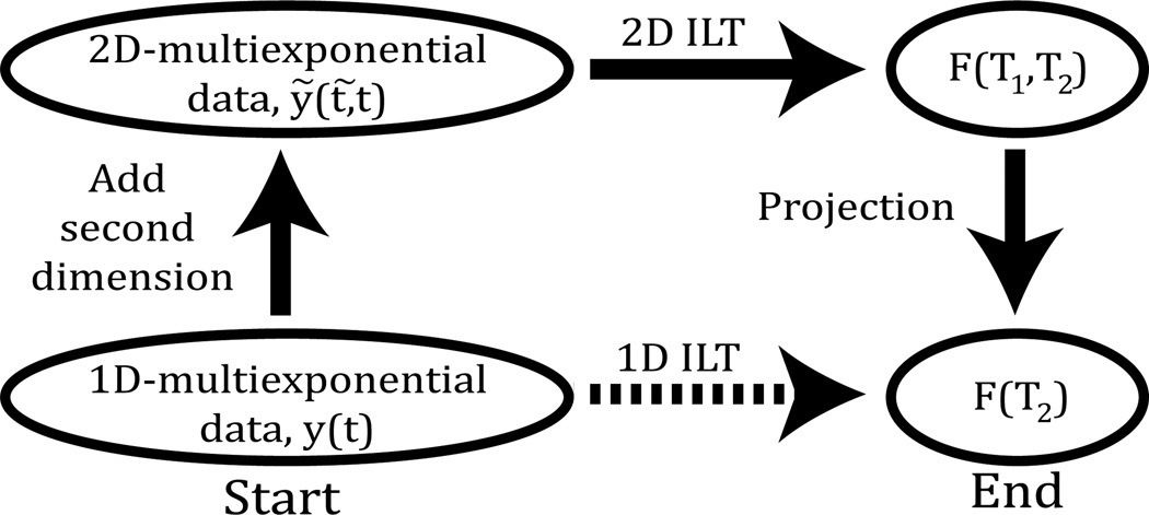
Expressions of identical form apply to other 2-dimensional relaxometry and hybrid experiments involving e.g. the pairs (T₂, T₂), and (T₂, D) [1, 6, 7]. In each case, a pulse sequence incorporating an indirectly-detected dimension with variable evolution time t̃ and a directly-acquired dimension parameterized by time is implemented. Through consideration of previous results on the stability of the ILT[2], and the fact that the span of multiplicatively separable functions mapping ℝ² → ℝ¹ is dense in the set of all such functions, we hypothesized that the 2D ILT would display greater accuracy and stability with respect to noise than the 1D ILT. Experiments yielding expressions of the form of Eq. 2 could then be used to determine F(T₂) through projection of the two-dimensional ILT onto the T₂ axis (Fig. 1).

Figure 1.

Dashed arrow indicates the 1D ILT of multicomponent decay data consisting of decaying exponentials, resulting in a T₂ histogram. The path traversed by the solid arrows introduces a second dimension to the data with a distinct, indirectly-sampled time variable t̃, representing e.g. the inversion time in a T₁ measurement. The T₂ histogram is then obtained by applying a 2D ILT to the two-dimensional data and then projecting the resulting T₁−T₂ histogram onto the T₂ axis.

The goal of the present work is to demonstrate that deriving the 1D ILT via the 2D ILT, that is, the path defined by the solid arrows in Fig. 1, yields much-improved results as compared to the direct calculation of the 1D ILT, that is, the dashed arrow path. We will refer to the 2D method as 2D ILT projection (2DILTP). Because ILT results improve with greater SNR, the comparison between the 1D and 2D approaches must be made on an equal-time basis. In the 2D experiment, acquisition time is proportional to the number of rows of data, m, acquired in the indirect dimension. Applying this additional time instead to signal-averaging a 1D acquisition would result in a $\sqrt{m}$ increase in SNR. Therefore, we compare results from a 2D dataset with results from a 1D dataset having a factor $\sqrt{m}$ higher SNR, or, equivalently, compare 1D to 2D experiments conducted with equal total acquisition time, where the repetition time was set to five times the T₁ of the slowest decaying component.

Simulation results, and experimental data from agarose gel phantom samples, will be presented. Two established methods for carrying out the ILT of a signal exhibiting multiexponential decay, non-negative least squares (NNLS) and non-linear least squares (NLLS), were investigated to determine the generalizability of our analyses. NNLS has the significant advantage of not requiring pre-specification of the number of underlying exponentials. In contrast, with NLLS, data points are fit to a pre-specified non-linear model function, which in our case is the sum of two decaying exponentials. Thus, NLLS requires a careful selection of signal model and reasonable initial estimates for fit parameters. NNLS suffers from much greater numerical instability and generally requires regularization to achieve reliable results. In addition, the flexibility of the NNLS approach leads to much more stringent signal-to-noise (SNR) requirements for stability and accuracy as compared to NLLS. Finally, even for a signal generated by two discrete relaxation components, regularized NNLS will return a histogram of T₂ values that may or may not resolve these components. In contrast, NLLS, by definition, returns and therefore resolves the number of components incorporated into the model, whether or not this accurately represents the system under study.

2. Methods

For NNLS, Eq. 1 was discretized with K−1 permissible values of T₂ and N time-domain data points

$$y(t_n)=\sum _{k=1}^{K-1}F(T_{2,k})e^{-t_n/T_{2,k}}+C,$$ (3)

where y(t_n) is the amplitude of the n^th echo and F_k = F(T_2,k) is the unknown T₂ distribution to be derived in the form of K−1 weights. This equation is discretized with A_nk as the N × K matrix representing the integral equation kernel. The final column accounts for a possible signal offset C. Thus, A_nk = e^−t_n/T_2,k, k ≤ K − 1, A_nK = 1, and the final entry in F is F_K = C. A Tikhonov regularization term controlled by the parameter μ was added in the usual manner[3, 4], so that the target function used for minimization with NNLS took the form:

$$X=\sum _{n=1}^N{\Vert \sum _{k=1}^K{A}_{nk}{F}_k-y_n\Vert }^2+\mu {\Vert \sum _{k=1}^K{F}_k\Vert }^2$$ (4)

This approach was extended in the conventional fashion for the two-dimensional relaxometry experiments defined by Eq. 2 [6]. The value of μ is determined so that regularization increases the misfit to the data

$${\chi }^2=\sum _{n=1}^N\sum _{k=1}^K\frac{{(A_{nk}{F}_k-y_n)}^2}{{\sigma }^2}$$ (5)

exhibited by the unregularized version of Eq. 4, that is, omitting the second term, by 1% [8]. Here, σ is the standard deviation (SD) of the noise in the data as determined after complete signal decay.

For NLLS, a two-component signal model consistent with the experimental data was assumed:

$$y(t_n)=M_0(f_1{e}^{-t_n/T_{2,1}}+f_2{e}^{-t_n/T_{2,2}})+\epsilon$$ (6)

for 1D relaxometry, and

$$\mathit{ỹ}({\mathit{t̃}}_m,t_n)=M_0(f_1{e}^{-t_n/T_{2,1}}{e}^{-{\mathit{t̃}}_m/T_{1,1}}+f_2{e}^{-t_n/T_{2,2}}{e}^{-{\mathit{t̃}}_m/T_{1,2}})+\epsilon$$ (7)

for 2D. Here, the f_i are component fractions satisfying f₁ + f₂ = 1, T_1,i and T_2,i are relaxation time constants, M₀ is the signal amplitude and ε represents additive Gaussian noise.

Numerical data, including those in plots, are presented as mean ±SD, except that error bars in Fig. 4 are standard error of the mean (SEM).

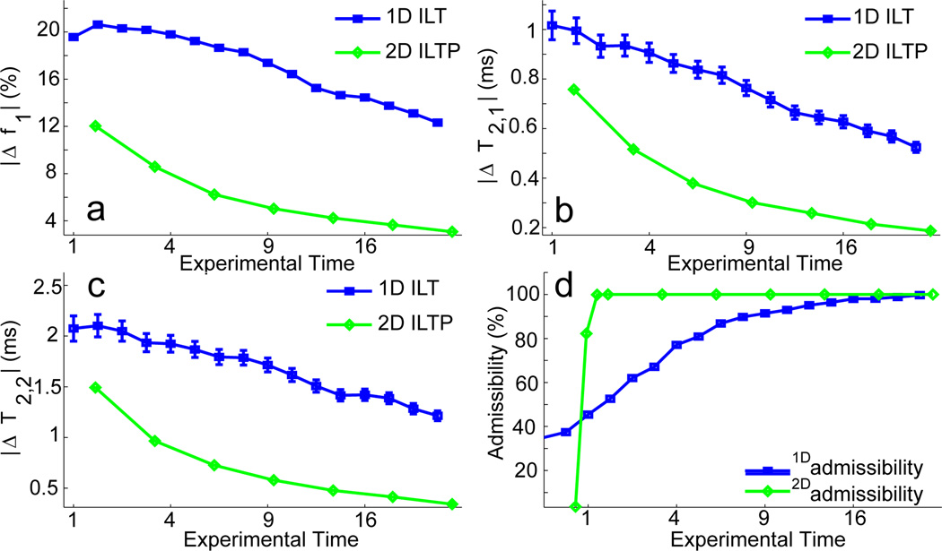
Figure 4.

Accuracy of NLLS-derived component parameters for the 1D ILT and for 2D ILTP. The abscissa is in arbitrary units, with the value of 1 corresponding to the experimental time for a single signal acquisition with SNR = 100 for 1D and SNR = 100sqrt6 for 2D. The vertical axes indicate the magnitude of the percent error in the indicated parameter over 1000 noise realizations. Due to the large sample size some of the standard error bars (± SEM) are not visible. a. Component fraction f₁; f₂ is related by f₂ = 1 − f₁. b & c. Accuracy of the T₂ values for the two components. d Fraction of noise realizations that yielded estimates within a factor of two for all parameters; such results were deemed ‘admissible’ (Fig. 4d).

3. Simulation Results

+Simulation and experimental results were obtained using a value of m = 6 for the number of points sampled in the indirect dimension for the 2D analysis. This was selected based on a Cramer-Rao lower bound calculation [9, 10, 11] (see supporting information), which indicated marginal further improvement in precision for m > 6.

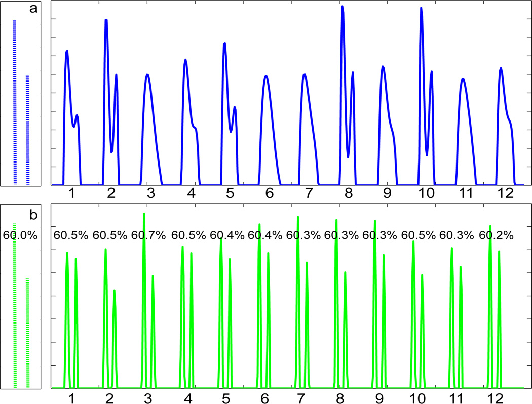
The sensitivity of the ILT to noise [2] is illustrated in Fig. 2. There is clearly a large variation in the morphology of the derived T₂ histogram from the 1D ILT (Fig. 2a); in fact, the two underlying signal components are resolved in only five out of the 12 noise realizations. Fig. 2b shows the results of the 2D analysis performed on an equal-time basis through adjustment of SNR. Both components are cleanly resolved for all noise realizations and component amplitudes are much more stable than in Fig. 2a. Similar results were obtained for the much more challenging problem of analysis of three underlying relaxation components with relaxation times and weights given by (T₂, weight) = (7 ms, 5%), (12 ms, 5%) and (50 ms, 90%) for 1D, and with T₁ values of 300 ms, 600 ms and 1500 ms incorporated for each component respectively in 2D. Again, resolution was consistently observed using the 2D approach but not with the 1D analysis, and quantification was much more accurate with 2DILTP (data not shown).

Figure 2.

The exact underlying form of a simulated distribution is shown on the left. The two components were defined by (T₂, weight) = (25 ms, 60%) and (35 ms, 40%). Relaxation data were generated from this and inverted using NNLS. Results from 12 different realizations of noise are shown on the right. a. Results from the 1D ILT (dashed arrow in Fig. 1). SNR = 15000. b. Results from 2DILTP (solid arrows in Fig. 1). T₁ values of 100 ms and 300 ms were assigned to the two components, respectively. $\mathrm{S}\mathrm{N}\mathrm{R}=15000\sqrt{6}~6000$. The numbers indicate the relative area of the larger component; all are within 1% of the correct value. Small variation in maxima is inherent to regularization.

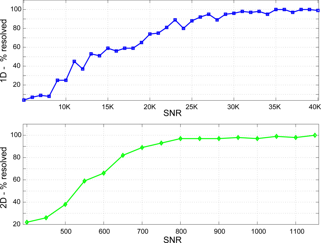
Using NNLS, we systematically investigated the reliability of 2DILTP for resolving two closely-spaced relaxation components with the same signal parameters as in Fig. 2. Results for a range of SNR values were obtained for 100 realizations of noise; components were considered resolved if the minimum of the T₂ distribution lying between the components was less than 90% of the amplitude of the smaller component. SNR values were incremented until the two components were consistently resolved. For the 1D ILT, SNR = 25000 was required in order that the components were resolved for 90% of the noise realizations (Fig. 3a), while a much more modest SNR~700 was required for the 2D approach (Fig. 3b). For the equal time comparison, the 1D ILT with $\mathrm{S}\mathrm{N}\mathrm{R}~\sqrt{6}\times 700=1700$ was unable to resolve the two components in any of the cases.

Figure 3.

Determination of resolution accuracy in T₂-dimension: Results for a range of SNR values were obtained for 100 realizations of noise with the same signal parameters as in Fig. 2. Components were considered resolved if the minimum of the T₂ distribution lying between the components was less than 90% of the amplitude of the smaller component. a 1D. b 2D.

Accuracy of component quantification was studied as a function of SNR using NLLS. A two-component signal was simulated; components for the 1D simulations were defined by (T₂, weight) = (15 ms, 60%) and (25 ms, 40%) and, for the 2D simulations, by (T₁, T₂, weight) = (100 ms, 15 ms, 60%) and (300 ms, 25 ms, 40%). Again 2DILTP demonstrated greatly improved results on an equal time basis (Fig. 4a–4d).

4. Gel Preparation & Data Acquisition

Two 5% w/w agarose gels were prepared with 0.05% and 0.15% CuSO4 by weight, respectively. The corresponding relaxation times and weights (T₁, T₂, weight) were (334 ms, 35 ms, 55%) and (122 ms, 27 ms, 45%). Two cylindrical samples, 4 mm in diameter, were extracted for each gel using a biopsy punch. The samples were placed in 5 mm NMR tubes, and the remaining volume of the sample tubes was filled with Fluorinert FC-770 in order to match the susceptibility of the agarose samples to improve shimming.

Experimental data were collected on a 9.4 T Bruker NMR spectrometer with an Avance III console and a Micro2.5 micro-imaging probe equipped with a 5 mm solenoidal coil. One-dimensional CPMG experiments were performed with echo time TE = 150 µs, repetition time TR = 4000 ms and number of echoes N = 1024. The data was signal-averaged 8 times for each 1D CPMG experiment. An inversion recovery CPMG experiment was conducted to observe T₁−T₂ correlations. The inversion recovery times were sampled logarithmically between 25–1500 ms with NI = 6 and a single scan was collected for each inversion experiment. Only even-numbered data points were used in post-processing. Computations were accelerated by decimating the T2 data sets according to the following: All even data points between 0–25 ms, every other even data point between 25–50 ms, every 4^th even data point between 50–100 ms, every 8^th even data point between 100–200 ms and every 16^th even data point between 200–400 ms were used for processing [8].

5. Experimental Results

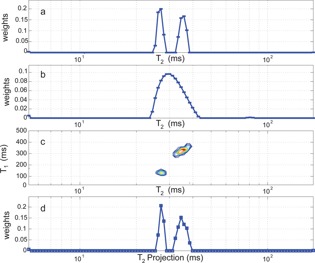
The sum of the T₂ distributions obtained from the two gels separately was taken as the gold standard for the combined gel sample (Fig. 5a). The relaxation times, as measured separately for each gel, and weight fractions, as measured from the combined histogram, were determined to be (T₁, T₂, weight) = (122 ms, 27 ms, 45%) and (334 ms, 35 ms, 55%).

Figure 5.

1D and 2D histograms for the two-component gel sample. a. T₂ distributions for individual gels combined into a single histogram. b. T₂ histogram for the two-component sample via the 1D ILT. c. T₁−T₂ histogram for the two-component sample via 2D ILT. d. T₂ projection of the T₁−T₂ histogram.

1D NNLS analysis of the signal obtained from the combined gel sample (Fig. 5b) reveals a broad component spanning T₂ ~ 25 – 45 ms and a much smaller second component with T₂ ~ 80 ms. This clearly does not resemble the gold standard histogram (Fig.5a). The histogram obtained from T₁−T₂ 2D ILT analysis of the combined sample with the same experimental time as the 1D experiment is shown in Fig. 5c. The components obtained by projection of the 2D histogram onto the T₂ axis (Fig. 5d) are characterized by (T2, weight) = (27 ms, 43%) and (36 ms, 57%); all values are within < 5% of the gold standard histogram. The T₁ histogram resulting from projection onto the T₁ axis likewise accurately reflects the T₁ values of the sample.

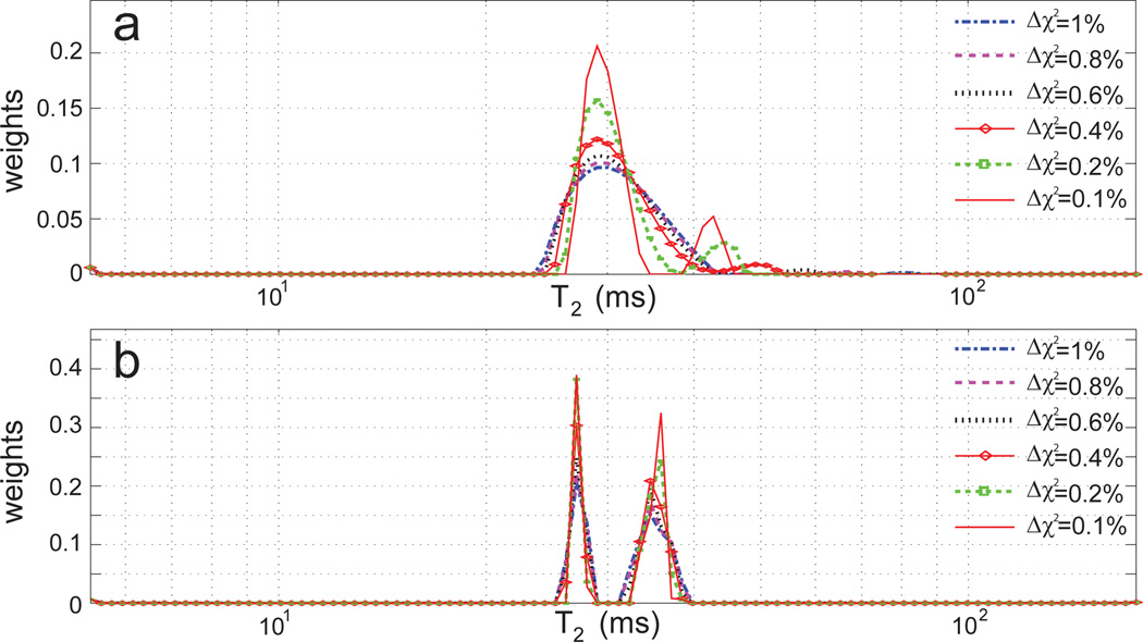
Fig. 5b was obtained with our standard criterion for regularization to result in a 1% increase in χ². However, the 1D ILT results are highly dependent upon regularization. Fig. 6a shows this for the two-component agarose gel. The dominant histogram component is broadened with increasing regularization, which also leads to the loss of the smaller of the two components. The two distinct components present when the least amount of regularization, Δχ² = 0.1%, is used are characterized by (T₂, weight) = (29 ms, 85%) and (43 ms, 15%); these values are very different from the gold standard results (Fig. 5a). The position of the smaller component at the longer T₂ value varies greatly with regularization. This problematic dependence of the 1D ILT on regularization is well-known[5].

Figure 6.

a. 1D ILT results for the two-component gel sample with varying degrees of regularization. b. Corresponding 2DILTP results.

In contrast, results of 2DILTP are much less dependent upon the degree of regularization (Fig. 6b). The morphology of the T₂ histogram is much more stable to the choice of Δχ² and accuracy is much more consistent. The component positions are stable and the number of components present is correctly determined for all degrees of regularization.

6. Discussion

There is a vast literature on the numerical solution to Eq. 1 and related Fredholm equations of the first kind[2, 5]. Here, we have demonstrated the marked increase in reliability and reproducibility of recovering the unknown one-dimensional function F(T₂) that results from performing a conventional 2D relaxometry experiment followed by 2D inverse Laplace transformation and projection, as compared to 1D relaxometry using the 1D inverse Laplace transformation. We considered cases in which F(T₂) is equal to the sum of delta functions, as shown by our simulation results, or is comprised of narrow histogram components, as shown by our experimental results. Our analyses indicate that similar results are found for more general forms of F(T₂), and, potentially, for different forms of the integral kernel, such as a stretched exponential. The introduction of the second dimension is made possible through the capabilities of NMR spectroscopy, so that this does not represent a general mathematical approach to improving the properties of the ILT. However, it may be of considerable utility in NMR relaxometry and in other experimental modalities in which a second dimension can be introduced.

The principle of 2DILTP was illustrated by comparing 1D T₂ relaxometry with 2D T₁−T₂ relaxometry followed by projection. However, the results are equally applicable to other integral kernels of the form of Eq. 2, with the choice of physical parameters for the direct and indirect dimensions depending upon the sample and the experimental conditions. Examples of particular interest may include (T₂, D), ($T_2^{*}$, D) or (T₂, MT), where MT denotes magnetization transfer ratio rate. This greatly extends the range of potential application of 2DILTP; the values of the MR parameters describing underlying signal components are intrinsic sample properties, so different indirect dimension parameters may be more well-suited than others for the 2DILTP in particular settings. Selection of an appropriate indirect dimension will require some degree of prior knowledge of sample characteristics.

In the present work, the greatly improved stability and accuracy of the 2DILTP as compared to the 1D ILT required that the ratio of the T1 relaxation times in the indirect dimension was greater than approximately 2. This value will depend upon SNR and the properties of the T₂ histogram itself, defined by the number of, separation between, and relative amplitudes of the components.

While this work may clearly be extended to dimensions greater than 2, this may be limited both by experimental time and by the availability of parameters that are well-separated in the indirect dimensions. Finally, in our analysis, the two-dimensional histogram was projected on the directly detected dimension. This was done in order to compare the 1D ILT to 2DILTP. In fact, however, the 2D histogram has much greater information content than its 1D projections. Thus, another view of our results is that in addition to the greater separation of components intrinsic to 2D experiments, the 2D histogram itself is substantially more stable and accurate than would be the 1D histograms obtained separately for the parameters defining the direct and indirect dimensions.

Highlights.

We propose a method of stabilizing the inverse Laplace transform of multiexponential NMR signals.

We examine simulated and experimental multiexponential NMR relaxation datasets.

Our method is based on conventional 2D relaxometry followed by 1D projection.

We compare these projections with 1D results on an equal experimental time basis.

We find markedly improved stability, accuracy, and insensitivity to regularization.

References

- 1.English AE, Whittall KP, Joy MLG, Henkelman RM. Quantitative two-dimensional time correlation relaxometry. Magnetic Resonance in Medicine. 1991;22(2):425–434. doi: 10.1002/mrm.1910220250. [DOI] [PubMed] [Google Scholar]
- 2.McWhirter JG, Pike ER. On the numerical inversion of the laplace transform and similar fredholm integral equations of the first kind. Journal of Physics A: Mathematical and General. 1978;11(9):1729. [Google Scholar]
- 3.Hansen PC. Discrete inverse problems : insight and algorithms. Society for Industrial and Applied Mathematics. 2010 [Google Scholar]
- 4.Lawson CL, Hanson RJ. Solving least squares problems. Prentice-Hall; 1974. [Google Scholar]
- 5.Murli A, Cuomo S, D’Amore L, Galletti A. Numerical regularization of a real inversion formula based on the laplace transform’s eigenfunction expansion of the inverse function. Inverse Problems. 2007;23(2):713–731. [Google Scholar]
- 6.Saab G, Thompson RT, Marsh GD, Picot PA, Moran GR. Two-dimensional time correlation relaxometry of skeletal muscle in vivo at 3 tesla. Magnetic Resonance in Medicine. 2001;46(6):1093–1098. doi: 10.1002/mrm.1304. [DOI] [PubMed] [Google Scholar]
- 7.Song YQ, Zielinski L, Ryu S. Two-dimensional nmr of diffusion systems. Physical Review Letters. 2008;100(24):4. doi: 10.1103/PhysRevLett.100.248002. [DOI] [PubMed] [Google Scholar]
- 8.Graham SJ, Stanchev PL, Bronskill MJ. Criteria for analysis of multicomponent tissue t-2 relaxation data. Magnetic Resonance in Medicine. 1996;35(3):370–378. doi: 10.1002/mrm.1910350315. [DOI] [PubMed] [Google Scholar]
- 9.Anastasiou A, Hall LD. Optimisation of t-2 and m-0 measurements of bi-exponential systems. Magnetic Resonance Imaging. 2004;22(1):67–80. doi: 10.1016/j.mri.2003.05.005. [DOI] [PubMed] [Google Scholar]
- 10.Cramer H. Mathematical methods of statistics. Princeton university press; 1946. [Google Scholar]
- 11.Rao CR. Information and the accuracy attainable in the estimation of statistical parameters. Bull. Calcutta Math. Soc. 1945;(37):81–91. [Google Scholar]
Associated Data
This section collects any data citations, data availability statements, or supplementary materials included in this article.