Quantification of Drive-Response Relationships Between Residues During Protein Folding

Abstract

Mutual correlation and cooperativity are commonly used to describe residue-residue interactions in protein folding/function. However, these metrics do not provide any information on the causality relationships between residues. Such drive-response relationships are poorly studied in protein folding/function and difficult to measure experimentally due to technical limitations. In this study, using the information theory transfer entropy (TE) that provides a direct measurement of causality between two times series, we have quantified the drive-response relationships between residues in the folding/unfolding processes of four small proteins generated by molecular dynamics simulations. Instead of using a time-averaged single TE value, the time-dependent TE is measured with the Q-scores based on residue-residue contacts and with the statistical significance analysis along the folding/unfolding processes. The TE analysis is able to identify the driving and responding residues that are different from the highly correlated residues revealed by the mutual information analysis. In general, the driving residues have more regular secondary structures, are more buried, and show greater effects on the protein stability as well as folding and unfolding rates. In addition, the dominant driving and responding residues from the TE analysis on the whole trajectory agree with those on a single folding event, demonstrating that the drive-response relationships are preserved in the non-equilibrium process. Our study provides detailed insights into the protein folding process and has potential applications in protein engineering and interpretation of time-dependent residue-based experimental observables for protein function.

INTRODUCTION

Protein folding is one of the fundamental problems in biosciences. Different parts of a protein may have long-range interactions and fold in a concerted way. Such cooperative folding is considered to be essential to prevent the formation of partially unfolded structures that leads to aggregation.^1-2 In terms of specific residue-residue interactions, it is possible to measure their correlations experimentally using NMR spectroscopy.^3-5 Computational methods such as molecular dynamics (MD) simulations and anisotropic network model also provide valuable information about the intrinsic cooperativity in proteins’ folding.^6-8 Pearson correlation and mutual information (MI) are two common measures to quantify the correlations. Specifically, MI incorporates both linear and nonlinear correlations and has been used in studying correlated motions of proteins.^9-12 However, one defect of these measures is that they are symmetric and thus it is not possible to distinguish one residue from another in a correlated pair. Knowing the directive interaction (i.e., the drive-response relationship) between residues is not only of theoretical interest, but also can provide guidance in protein engineering.

A theoretic metric that can determine the drive-response relationships between residues is the information theory transfer entropy (TE) proposed by Schreiber.¹³ TE quantifies the information flow from the past of one time series to the future of another time series. It has been used in finance¹⁴ and mostly in neuroscience to deduce the connection between neurons.^15-16 Recently, TE has been used in MD simulation trajectory analysis to elucidate the information flow in a transcription factor Ets-1.¹⁷ Through the analysis of the simulation trajectories of the apo and holo states, the binding of DNA to H1 helix of Ets-1 appears to drive the correlated motion of the inhibitory helix HI-1 via a relay helix. The same method was applied to the autoactivation of extracellular signal-regulated kinases 1 and 2,¹⁸ revealing how the helix-C at N-domain drives the fluctuation of the activation lip that may lead to activation. Another application of TE analysis is to identify important order parameters from MD simulations,^19-20 so that protein conformational changes can be better described by the change of these order parameters compared to those based on principle component analysis. These studies demonstrate that, when applied to MD simulation trajectory analysis, TE can be a valuable method in understanding the functional motions of proteins. However, statistical significance of calculated TE values is not clearly addressed in these studies.^17-20 Since the calculated TE values are often very small, it is critical to use well-defined statistical significance analysis to warrant wide applications of the TE analysis in both computational and experimental studies.

In this study, we apply the TE analysis to quantify the drive-response relationships between residues in the folding/unfolding processes of four small proteins generated by MD simulations. While it is well recognized that hydrophobic interactions are the driving force in protein folding,²¹ to the best of our knowledge, to what extent each residue drives/responds to each other has not been studied before. In addition, the identified driving and responding residues are compared with those correlated residues identified by mutual information analysis; examined by the general properties such as secondary structure and solvent accessible surface area; and characterized by their effects on the protein stability as well as folding and unfolding rates. In terms of the computational and theoretical point of view, our study establishes statistical significance analysis of calculated TE values using simulation trajectories and determines if the stationary drive-response relationship is preserved in local, non-equilibrium events. Our understanding of protein function and underlying mechanisms of biologically important processes can be enriched by identifying residue-residue drive-response relationships through wide applications of TE analysis to MD simulations as well as time-dependent residue-based experimental observables.

MATERIALS AND METHODS

Theory

The all-atom folding trajectories were obtained from D. E. Shaw Research for their recent protein folding simulation study; the trajectories were saved every 200 ps and contained the coordinates of Cα atoms²². Of the 12 proteins simulated, Trp-cage, BBL, Villin, and BBA were selected for this study because these proteins had multiple folding/unfolding events. To obtain a time series for each residue, we used a residue-based Q-score, i.e., the fraction of native contacts formed for a specific residue. A native contact is counted when two Cα atoms are closer than 1.2 times their distance in the native structure.

TE is a measure that quantifies the information flow from the past of one time series y(t) to the future of another time series x(t) (Figure 1). It was formally described by Schreiber¹³ as

$$T{E}_{y\to x}=\sum p(x_{t+1},x_t^{(k)},y_t^{(l)})\log \frac{p(x_{t+1}\mid x_t^{(k)},y_t^{(l)})}{p(x_{t+1}\mid x_t^{(k)})}$$ (1)

where k and l are the embedding dimensions that are the number of steps to be included from the past, p() is the probability of one state, p(∣) is the conditional probability, and the summation is over all possible combinations of states. By simple manipulation, TE can also be written in terms of Shannon entropy, H (x) = −Σp(x_t) log p(x_t), which is the actual form used in the present calculations,

$$\begin{array}{lll}T{E}_{y\to x}& =& H(x_{t+1}\mid x_t^{(k)})-H(x_{t+1}\mid x_t^{(k)},y_t^{(l)})\\ & =& H(x_{t+1},x_t^{(k)})+H(x_t^{(k)},y_t^{(l)})-H(x_{t+1},x_t^{(k)},y_t^{(l)})-H(x_t^{(k)})\end{array}$$ (2)

where H(∣) is conditional Shannon entropy. Due to finite sample size of the time series, two independent series can have (statistically insignificant) non-zero TE. To remove this bias, the shuffling method was used to calculate the effective TE (TE^eff),^{14, 17} which is given by

$$T{E}_{y\to x}^{\mathit{eff}}=T{E}_{y\to x}-\frac{1}{N}\sum _{n=1}^{N}T{E}_{y_{\mathit{shuffled}}\to x}$$ (3)

where N is the number of shuffling, and should be set to a sufficiently large number.²³ We used 500 for all calculations in this study. Using TE^eff, a normalized directional index can be derived as

$$D_{y\to x}=\frac{T{E}_{y\to x}^{\mathit{eff}}}{H(x_{t+1}\mid x_t^{(k)})}-\frac{T{E}_{x\to y}^{\mathit{eff}}}{H(y_{t+1}\mid y_t^{(l)})}\in [-1,1]$$ (4)

where $H(x_{t+1}\mid x_t^{(k)})$ and $H(y_{t+1}\mid y_t^{(l)})$ are the maximal TE. A positive D value indicates information flow from y(t) to x(t), and vice versa for a negative value. For two completely independent time series, D_y→x and TE^eff are 0. Our implementation of TE was verified with three numerical systems (SI Section S1).

Figure 1.

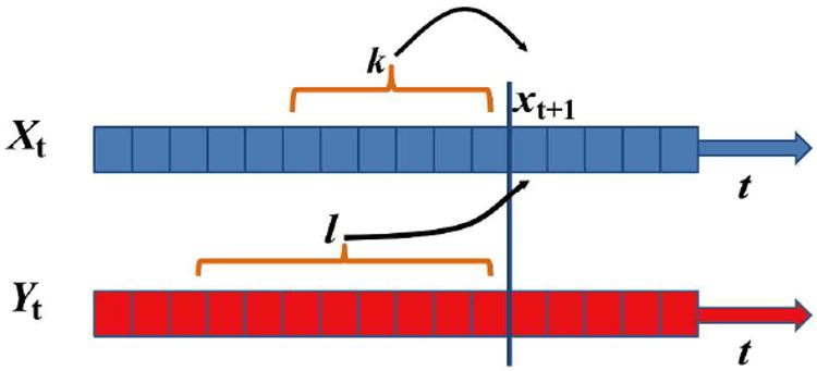
Schematic illustration of measuring TE. y(t) and x(t) are two time series. Let us assume that we try to predict the future of x(t), x_t+1, using the past k steps from x(t) and past l steps from y(t). TE is the difference in such predictions between using the past of x(t) only :wqand using the past of x(t) and y(t) together, and quantifies the information flow from y(t) to x(t).

MI quantifies the difference of information between two time series. For x(t) and y(t), MI is

$$\mathit{MI}(x,y)=H(x)+H(y)-H(x,y)$$ (5)

We used a normalized MI as

$$M{I}^{\prime }(x,y)=\sqrt{1-e^{-2\mathit{MI}(x,y)}}$$ (6)

which ranges between 0 and 1.²⁴

Practical computational considerations

From the practical computational point of view, several parameters affect the calculated TE values and must be determined carefully. The first one is symbolization, which is to map the time series to a finite set of symbols (i.e., discrete values or states) so that one can calculate the probability of having each symbol. Too many symbols result in poor estimation of probability density, while too few symbols usually fail to capture the dynamics of the system. One method of symbolization is using the relative rank of each data point.²⁵ This method may reduce the state space under certain circumstances. A more intuitive method is to partition the data to several ranges and use the range index as symbol. As the residue Q-score has finite discrete states in nature, we directly used the number of native contacts formed for each residue as the symbol, which resulted in 5 symbols per residue on average.

The second crucial parameter is the embedding dimension k and l in Equation (1) and Figure 1. The optimal dimension is system-dependent and difficult to be generalized. Although the false nearest-neighbors method has been used by others,^{17, 26} it does not guarantee the best solution and converges to (unrealistic) high dimensions in the semi-stationary series studied here. High dimensions cause problems in probability estimation as the state space is proportional to n^k+l+1 in Equation (2), where n is the average number of symbols per residue. With this in mind, we used low dimensions from 1 to 4 to examine if two window lengths 20,000 (4 μs simulation time) and 50,000 (10 μs) were sufficient to obtain meaningful time-dependent TE values. For each window size, we used the half of its length to slide over the whole trajectory. As TE can only be applied to stationary process, for each window along the simulation time, we used the augmented Dickey–Fuller method²⁷ to test its stationarity. The final results are based on embedding dimension 1 for both k and l because different dimension from 1 to 4 does not change the dominant driving and responding residues (data not shown). The time-dependent TE values were calculated with the window size of 10 μs (for Trp-cage, BBL and BBA) and 4 μs (for Villin) as these window sizes showed 0 percent non-stationary windows along the simulation time. In the single folding (non-equilibrium) events, it is more difficult to use a window that is small enough to be stationary while large enough to contain statistically meaningful data points. We finally used a window size of 2 μs (i.e., 10,000 data points), which has 1.4% and 2.6% non-stationary windows for the two single folding events of BBL.

Finally, for each D_y→x value in Equation (4), it is highly desirable to assess its significance using statistical test. This is particularly important because D_y→x is generally very small in magnitude (below 0.1), so that it is difficult to evaluate its statistical significance even with the shuffling method in Equation (3). Therefore, we calculated the p-value using z-test against the random distributions of D_y→x from shuffling. A cutoff of 0.1 was first applied to D_y→x values to remove residue pairs that had small drive-response interactions, and then a p-value cutoff of 0.05 was used to filter out a considerable number of pairs that were not significant (Table 1).

Table 1.

Number of drive-response residue pairs with and without the p-value cutoff of 0.05 for the analysis of whole trajectories of the test proteins.

p-value Cutoff	Trp-cage	BBL	Villin	BBA
Yes	36	17	16	8
No	82	149	133	42

RESULTS AND DISUCSSION

We applied the TE analysis to folding processes of four small proteins (Trp-cage, BBL, Villin, and BBA), whose trajectories were obtained from the recent protein folding simulations by Lindorff-Larsen et al. in D. E. Shaw Research,²² and the simulation lengths were between 100 and 200 μs. Briefly, a residue Q-score was calculated for each residue along simulation time, and TE were calculated between every residue pair in a time-dependent manner. The normalized directional index D_y→x in Equation (4), after a threshold cutoff and significance test (see Materials and Methods), indicates whether residue y drives (D_y→x >0) or responds to (D_y→x <0) residue x. The correspondence between the Q-score and D_y→x values is remarkable (Figure 2), indicating that transfer of information entropy generally happens upon folding and unfolding events.

Figure 2.

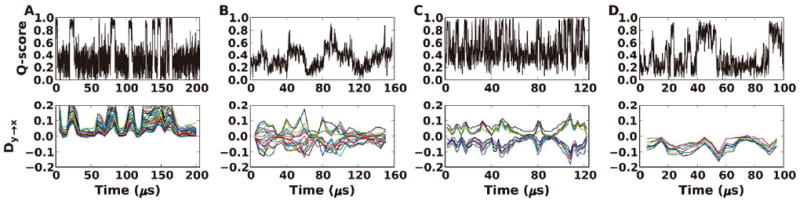
Time-dependent Q-score and D_y→x profiles of the whole folding trajectory for (A) Trp-cage, (B) BBL, (C) Villin, and (D) BBA. Different colors in the D_y→x profiles represent different residue pairs.

To elucidate the drive-response relationships between residues, we calculated the time-average D_y→x of each residue pair. Figure 3A (lower diagonal) shows the results of Trp-cage. Trp-cage is a small protein with only 20 amino acids that consists of an α-helix, a 3₁₀-helix, and a polyproline region at the C terminal (Figure 3B). Our results indicate that the folding of the polyproline region responds to the residues in the α-helix. The rationalization of this behavior is clear in terms of the Trp-cage structure (Figure 3B). The N terminal helix forms first and then drives the formation of tertiary contacts of the polyproline region. It has been suggested that the folding of local structure followed by tertiary contact formation is a general mechanism of protein folding,²² although the drive-response relationship can only be revealed by information analysis such as TE in this study. Notably, Trp-6, which is the most important residue in Trp-cage, is the dominant driver in our analysis as it drives 6 residues. The interactions between Trp-6 and 3₁₀-helix group as well as between Trp-6 and the polyproline region, which proved to be important in experimental and computational studies,^28-29 are also captured in the TE analysis.

Figure 3.

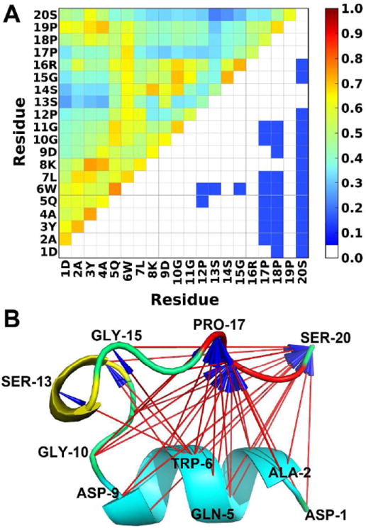
Driving and responding residues in Trp-cage folding/unfolding. (A) A driver-responder plot indicates a residue from x-axis drives (red) or responds to (blue) a residue from y-axis (lower-half triangle). Since the C-terminal residues respond to N-terminal residues in Trp-cage, no red color is shown. MI values, calculated from the whole trajectory, are colored based on the color-coding bar (upper-half triangle). MI values smaller than 0.05 are colored in white. (B) The structural view of the driving and responding residues. Arrows indicate driving interactions. α-helix in cyan, 3₁₀-helix in yellow, and polyproline region in red.

MI is a measure that quantifies the difference of information between two time series. To compare TE with MI, we also calculated MI for each residue pair of Trp-cage (Figure 3A upper diagonal). The residue-residue correlations from MI are quite different from TE. In TE, the helical residues and the polyproline residues are correlated, while in MI, the correlation exists between N and C terminals, between residue 9-11 and 15-16, and between the helical residues. The differences between MI and TE also exist in BBL, BBA, and Villin (Figure S2). Such differences arise from the fact that our MI calculation only takes into account concurrent events. In other words, MI only calculates the correlations for the events at the same time, while TE is able to incorporate the information from the past. A variation of MI, the time-delayed MI, which introduces a time lag to one of the series, is also able to capture causality in dynamic systems.^30-32 We applied time-delayed MI to the test proteins, but it did not reveal any drive/response interactions (SI Section S3).

Are there any general features of the driving and responding residues in folding and unfolding of proteins studied in this work? First, we check if a driving-responding relationship of a residue pair changes in time. A residue may drive another residue at one time and respond to the same residue at a later time. We counted the number of times D_y→x changes its sign in the four proteins and found that none of the residue pairs changed their driving-responding relationships. This result not only justifies the use of time-average D_y→x value to classify the drive-response relationship in Figure 3, but also suggests that residues play a constant role in the folding process. Second, we examine the relationship between the driving and responding residues and their locations in the context of protein structure. In Trp-cage, the driving residues are mostly in the buried helical region (Figure 3B). To examine whether this is a general feature, we calculated the secondary structures and relative solvent accessibility to each residue in the proteins. More than 70% of the driving residues are located in helix and sheet, but for the responding residues, the percentage of forming regular secondary structures is only 25% (Figure 4). For relative solvent accessibility to each residue, which is calculated as the percentage of the solvent accessible surface area (SASA) of a residue in the protein structure compared to that of a free residue, the driving residues have an average value of 38.2 ± 26.7%, while the responding residues have an average of 80.6 ± 31.1%. Thus, the driving residues are mostly buried at the hydrophobic core and have more regular secondary structures.

Figure 4.

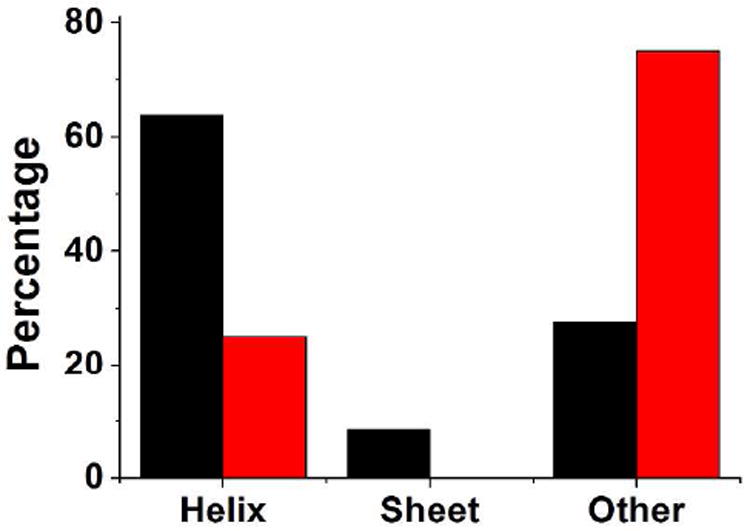
Percentages of different secondary structures of driving (black) and responding residues (red) from the test proteins

Is there any experimental support for the driving and responding residues identified by the TE analysis? Trp-6 in Trp-cage, which is the dominant driver, is already known to be of crucial importance to Trp-cage folding. For another protein BBL, a small protein with down-hill folding behavior under certain conditions, some experimental mutation data are available.^33-35 We compared the transition temperature (T_m), the folding rate (k_f), and the unfolding rate (k_u) before and after the driving and responding residues are mutated (Table 2). Mutations to driving residues V163, T159, D162, and I135 decrease T_m and k_f by 6.54-12.3% and 50.6-81.6%, and increase k_u by 181.8-1016.9%, respectively. Mutation to the responding residue A148 has much smaller effects. No point-mutation experimental data are available for Villin and BBA, but we found almost every residue has been mutated for protein L, and k_u and k_f were also measured.^36-37 As protein L has 61 residues and the folding process is not easy to simulate with all-atom simulations, we used coarse-grained GO-type model^38-39 to generate folding/unfolding trajectories (Figure S5). Using the same analysis, we identified the driving and responding residues and compared how k_f and k_u changed after mutations (Figure 5). Similar to BBL, mutations to driving residues have greater effects on k_f and k_u.

Table 2.

The effects of mutations of driving and responding residues on experimental denaturation midpoint (T_m), folding (k_f), and unfolding rates (k_u) of BBL. The experimental data are shown as percentage changes compared to wild type values. T_m, k_f, and k_u for wild type BBL are 327.3 K, 71,000 s^-1, and 770 s^-1.

Mutation to Driving Residues				Mutation to Responding Residues
Mutation	Tm	kf	ku	Mutation	Tm	kf	ku
V163A	-8.04	-72.0	1016.9	A148G	-1.7	-38.1	-24.7
T159S	-6.54	-60.3	181.8
D162N	-12.3	-81.6	324.6
I135A	-6.54	-50.6	459.7

Figure 5.

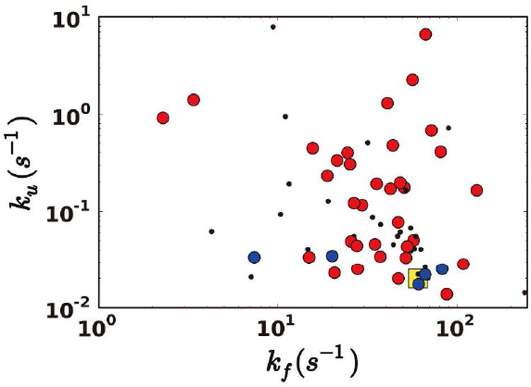
Effects of mutations to driving and responding residues in protein L. Mutations to driving residues in red circles, to responding residues in blue circles, others in black dots, and the wild type values in yellow square.

So far, we focus on the whole folding trajectories with multiple folding events as a stationary process. To see if the drive-response relationships are preserved in single folding events (i.e., non-equilibrium process), we extracted two folding events from the trajectory of BBL (Figure 6): one from 60 to 90 μs and the other from 125 to 150 μs. It should be noted that the TE analysis can only be applied to a stationary process,¹³ so it is necessary to use windowing method to partition the original single folding event to several stationary windows (see Materials and Methods). The D_y→x profiles have correspondence with Q-score, but are less evident. In terms of driving and responding residues, compared to the results from the whole trajectory (Figure 7A), the two single folding events are noisier and thus have more drive-response pairs (Figure 7B, C). However, when considering the pairs shared by the two single folding events, it is clear that the dominant responding residue A148 from the whole trajectory is still preserved (Figure 7D; red in lower-half triangle). Thus, the main characters of the drive-response relationships from the whole trajectories are still captured in the single folding events.

Figure 6.

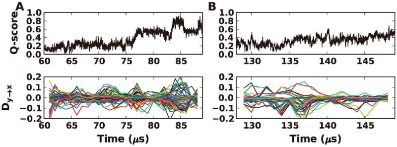
Q-score and D_y→x profiles of two single folding events for BBL

Figure 7.

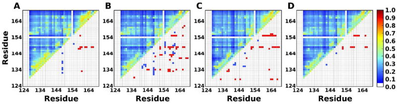
Driving and responding residues for BBL determined from (A) the whole trajectory and (B and C) two single folding events. (D) The shared drive-response residues and average MI from (B) and (C). The color schemes are the same as in Figure 3.

CONCLUDING REMARKS

In this study, we applied the TE analysis to the folding simulation trajectories of four small proteins, with the aim of identifying the drive-response relationship between residues and extending the TE analysis in a time-dependent manner with test of statistical significance. Deciphering such relationships is interesting in a theoretical point of view and can only be carried out with information analysis such as TE. We find excellent correspondence between the folding process and the TE values between residues. Upon folding and unfolding, a large amount of information entropies is transferred between residues. Compared to responding residues, the driving residues are mostly buried at the hydrophobic core and form more regular secondary structures. They also have greater impacts on the protein stability as well as folding and unfolding rates. We also carried out the analysis on two single folding events from BBL and illustrate that the dominant responding residues from the whole trajectory are preserved in the single events.

The TE analysis can only be applied to a stationary process, i.e., the average and standard deviation of the time series do not change over time. For a non-stationary process, using windowing method to cut the whole series into several segments could bypass this problem in principle. In analyzing the whole trajectories, we used two window sizes of 4 and 10 μs, and carried out the stationary test to make sure that each window was stationary. In the single folding events, it is more difficult to use a window that is small enough to fulfill the stationary requirement while large enough to contain sufficient data points. We ended up with a window size of 2 μs, a compromise between the aforementioned two requirements, which resulted in 1.4% and 2.6% non-stationary windows for the two single folding events. The agreement of the dominant responding residues from the single folding events and the whole trajectories suggests that this small percentage of non-stationary window might be negligible. Another interesting observation is the time symmetric properties of the drive-response relationship. In the whole folding trajectories, as the trajectories are time reversible, we do not expect any change between results calculated from the forward and backward time series. In the single folding events, even if residue A drives residue B in the forward (folding) process, residue B does not necessarily drive residue A in the backward (unfolding) process. The causality relationship of two residues depends not only on the sequential events, but also on the direction of information flow between them.

TE is applicable to any stationary time series in general. However, to get meaningful insights from the TE analysis, statistical significance and stationary tests should be performed carefully. The windowing method allows us to look at the causality in a time-dependent manner when time evolution of the system is of interest; it also provides an effective way to get around the stationary problem for non-stationary processes. As many processes in biology are non-equilibrium in nature and the experimental observables are thus mostly non-stationary, the wide applications of the TE analysis to such experimental observables are expected to reveal the underlying mechanisms of biologically important processes.

References

- 1.Clark LA. Protein aggregation determinants from a simplified model: cooperative folders resist aggregation. Protein Sci. 2005;14:653–662. doi: 10.1110/ps.041017305. [DOI] [PMC free article] [PubMed] [Google Scholar]
- 2.Monsellier E, Chiti F. Prevention of amyloid-like aggregation as a driving force of protein evolution. EMBO Rep. 2007;8:737–742. doi: 10.1038/sj.embor.7401034. [DOI] [PMC free article] [PubMed] [Google Scholar]
- 3.Luque I, Leavitt SA, Freire E. The linkage between protein folding and functional cooperativity: two sides of the same coin? Annu Rev Biophys Biomol Struct. 2002;31:235–256. doi: 10.1146/annurev.biophys.31.082901.134215. [DOI] [PubMed] [Google Scholar]
- 4.Lundstrom P, Mulder FA, Akke M. Correlated dynamics of consecutive residues reveal transient and cooperative unfolding of secondary structure in proteins. Proc Natl Acad Sci U S A. 2005;102:16984–16989. doi: 10.1073/pnas.0504361102. [DOI] [PMC free article] [PubMed] [Google Scholar]
- 5.Osawa M, Takeuchi K, Ueda T, Nishida N, Shimada I. Functional dynamics of proteins revealed by solution NMR. Curr Opin Struct Biol. 2012;22:660–669. doi: 10.1016/j.sbi.2012.08.007. [DOI] [PubMed] [Google Scholar]
- 6.Pan H, Lee JC, Hilser VJ. Binding sites in Escherichia coli dihydrofolate reductase communicate by modulating the conformational ensemble. Proc Natl Acad Sci U S A. 2000;97:12020–12025. doi: 10.1073/pnas.220240297. [DOI] [PMC free article] [PubMed] [Google Scholar]
- 7.Bahar I, Lezon TR, Yang LW, Eyal E. Global Dynamics of Proteins: Bridging Between Structure and Function. Annu Rev Biophys. 2010;39:23–42. doi: 10.1146/annurev.biophys.093008.131258. [DOI] [PMC free article] [PubMed] [Google Scholar]
- 8.Lane TJ, Shukla D, Beauchamp KA, Pande VS. To milliseconds and beyond: challenges in the simulation of protein folding. Curr Opin Struct Biol. 2012;23:58–65. doi: 10.1016/j.sbi.2012.11.002. [DOI] [PMC free article] [PubMed] [Google Scholar]
- 9.Lange OF, Grubmuller H. Generalized correlation for biomolecular dynamics. Proteins. 2006;62:1053–1061. doi: 10.1002/prot.20784. [DOI] [PubMed] [Google Scholar]
- 10.Sedeh RS, Fedorov AA, Fedorov EV, Ono S, Matsumura F, Almo SC, Bathe M. Structure, evolutionary conservation, and conformational dynamics of Homo sapiens fascin-1, an F-actin crosslinking protein. J Mol Biol. 2010;400:589–604. doi: 10.1016/j.jmb.2010.04.043. [DOI] [PMC free article] [PubMed] [Google Scholar]
- 11.Rivalta I, Sultan MM, Lee NS, Manley GA, Loria JP, Batista VS. Allosteric pathways in imidazole glycerol phosphate synthase. Proc Natl Acad Sci U S A. 2012;109:8366–8367. doi: 10.1073/pnas.1120536109. [DOI] [PMC free article] [PubMed] [Google Scholar]
- 12.Roy A, Post CB. Detection of Long-Range Concerted Motions in Protein by a Distance Covariance. J Chem Theory Comput. 2012;8:3009–3014. doi: 10.1021/ct300565f. [DOI] [PMC free article] [PubMed] [Google Scholar]
- 13.Schreiber T. Measuring information transfer. Phys Rev Lett. 2000;85:461–464. doi: 10.1103/PhysRevLett.85.461. [DOI] [PubMed] [Google Scholar]
- 14.Marschinski R, Kantz H. Analysing the information flow between financial time series - An improved estimator for transfer entropy. Eur Phys J B. 2002;30:275–281. [Google Scholar]
- 15.Gourevitch B, Eggermont JJ. Evaluating information transfer between auditory cortical neurons. J Neurophysiol. 2007;97:2533–2543. doi: 10.1152/jn.01106.2006. [DOI] [PubMed] [Google Scholar]
- 16.Buehlmann A, Deco G. Optimal information transfer in the cortex through synchronization. PLoS Comput Biol. 2010;6 doi: 10.1371/journal.pcbi.1000934. [DOI] [PMC free article] [PubMed] [Google Scholar]
- 17.Kamberaj H, van der Vaart A. Extracting the causality of correlated motions from molecular dynamics simulations. Biophys J. 2009;97:1747–1755. doi: 10.1016/j.bpj.2009.07.019. [DOI] [PMC free article] [PubMed] [Google Scholar]
- 18.Barr D, Oashi T, Burkhard K, Lucius S, Samadani R, Zhang J, Shapiro P, MacKerell AD, van der Vaart A. Importance of domain closure for the autoactivation of ERK2. Biochemistry. 2011;50:8038–8048. doi: 10.1021/bi200503a. [DOI] [PMC free article] [PubMed] [Google Scholar]
- 19.Perilla JR, Woolf TB. Towards the prediction of order parameters from molecular dynamics simulations in proteins. J Chem Phys. 2012;136:164101. doi: 10.1063/1.3702447. [DOI] [PMC free article] [PubMed] [Google Scholar]
- 20.Perilla JR, Leahy DL, Woolf TB. Molecular dynamics simulations of transitions for ECD Epidermal Growth Factor Receptors show key differences between human and drosophila forms of the receptors. Proteins. 2013 doi: 10.1002/prot.24257. [DOI] [PMC free article] [PubMed] [Google Scholar]
- 21.Dill KA. Dominant forces in protein folding. Biochemistry. 1990;29:7133–7155. doi: 10.1021/bi00483a001. [DOI] [PubMed] [Google Scholar]
- 22.Lindorff-Larsen K, Piana S, Dror RO, Shaw DE. How fast-folding proteins fold. Science. 2011;334:517–520. doi: 10.1126/science.1208351. [DOI] [PubMed] [Google Scholar]
- 23.Weil P, Hoffgaard F, Hamacher K. Estimating sufficient statistics in co-evolutionary analysis by mutual information. Comput Biol Chem. 2009;33:440–444. doi: 10.1016/j.compbiolchem.2009.10.003. [DOI] [PubMed] [Google Scholar]
- 24.Joe H. Relative Entropy Measures of Multivariate Dependence. J Am Statist Assoc. 1989;84:157–164. [Google Scholar]
- 25.Staniek M, Lehnertz K. Symbolic transfer entropy. Phys Rev Lett. 2008;100:158101. doi: 10.1103/PhysRevLett.100.158101. [DOI] [PubMed] [Google Scholar]
- 26.Cellucci CJ, Albano AM, Rapp PE. Comparative study of embedding methods. Phys Rev E. 2003;67:066210. doi: 10.1103/PhysRevE.67.066210. [DOI] [PubMed] [Google Scholar]
- 27.Said SE, Dickey DA. Testing for Unit Roots in Autoregressive-Moving Average Models of Unknown Order. Biometrika. 1984;71:599–607. [Google Scholar]
- 28.Barua B, Lin JC, Williams VD, Kummler P, Neidigh JW, Andersen NH. The Trp-cage: optimizing the stability of a globular miniprotein. Protein Eng Des Sel. 2008;21:171–185. doi: 10.1093/protein/gzm082. [DOI] [PMC free article] [PubMed] [Google Scholar]
- 29.Hu Z, Tang Y, Wang H, Zhang X, Lei M. Dynamics and cooperativity of Trp-cage folding. Arch Biochem Biophys. 2008;475:140–147. doi: 10.1016/j.abb.2008.04.024. [DOI] [PubMed] [Google Scholar]
- 30.Paulus MP. Long-range interactions in sequences of human behavior. Phys Rev E. 1997;55:3249–3256. [Google Scholar]
- 31.Chaitankar V, Ghosh P, Perkins EJ, Gong P, Zhang C. Time lagged information theoretic approaches to the reverse engineering of gene regulatory networks. BMC Bioinformatics. 2010;11(Suppl 6):S19. doi: 10.1186/1471-2105-11-S6-S19. [DOI] [PMC free article] [PubMed] [Google Scholar]
- 32.Wilmer A, de Lussanet M, Lappe M. Time-delayed mutual information of the phase as a measure of functional connectivity. PLoS One. 2012;7:e44633. doi: 10.1371/journal.pone.0044633. [DOI] [PMC free article] [PubMed] [Google Scholar]
- 33.Cho SS, Weinkam P, Wolynes PG. Origins of barriers and barrierless folding in BBL. Proc Natl Acad Sci U S A. 2008;105:118–123. doi: 10.1073/pnas.0709376104. [DOI] [PMC free article] [PubMed] [Google Scholar]
- 34.Neuweiler H, Sharpe TD, Johnson CM, Teufel DP, Ferguson N, Fersht AR. Downhill versus barrier-limited folding of BBL 2: mechanistic insights from kinetics of folding monitored by independent tryptophan probes. J Mol Biol. 2009;387:975–985. doi: 10.1016/j.jmb.2008.12.056. [DOI] [PubMed] [Google Scholar]
- 35.Neuweiler H, Sharpe TD, Rutherford TJ, Johnson CM, Allen MD, Ferguson N, Fersht AR. The folding mechanism of BBL: Plasticity of transition-state structure observed within an ultrafast folding protein family. J Mol Biol. 2009;390:1060–1073. doi: 10.1016/j.jmb.2009.05.011. [DOI] [PubMed] [Google Scholar]
- 36.Kim DE, Fisher C, Baker D. A breakdown of symmetry in the folding transition state of protein L. J Mol Biol. 2000;298:971–984. doi: 10.1006/jmbi.2000.3701. [DOI] [PubMed] [Google Scholar]
- 37.Naganathan AN, Munoz V. Insights into protein folding mechanisms from large scale analysis of mutational effects. Proc Natl Acad Sci U S A. 2010;107:8611–8616. doi: 10.1073/pnas.1000988107. [DOI] [PMC free article] [PubMed] [Google Scholar]
- 38.Go N. Theoretical studies of protein folding. Annu Rev Biophys Bioeng. 1983;12:183–210. doi: 10.1146/annurev.bb.12.060183.001151. [DOI] [PubMed] [Google Scholar]
- 39.Qi Y, Huang Y, Liang H, Liu Z, Lai L. Folding simulations of a de novo designed protein with a betaalphabeta fold. Biophys J. 2010;98:321–329. doi: 10.1016/j.bpj.2009.10.018. [DOI] [PMC free article] [PubMed] [Google Scholar]
Associated Data
This section collects any data citations, data availability statements, or supplementary materials included in this article.