

Abstract
We consider multiple diseases spreading in a static configuration model network. We make standard assumptions that infection transmits from neighbor to neighbor at a disease-specific rate and infected individuals recover at a disease-specific rate. Infection by one disease confers immediate and permanent immunity to infection by any disease. Under these assumptions, we find a simple, low-dimensional ordinary differential equations model which captures the global dynamics of the infection. The dynamics depend strongly on initial conditions. Although we motivate this Rapid Communication with infectious disease, the model may be adapted to the spread of other infectious agents such as competing political beliefs, or adoption of new technologies if these are influenced by contacts. As an example, we demonstrate how to model an infectious disease which can be prevented by a behavior change.
a. Introduction
Many important dynamical systems involve the spread of some process through a network [1–3]. Our ability to understand the systems is complicated by a lack of analytic models, limiting our understanding of the dynamics. Particularly when competing processes are occurring in the network, the final outcome may be highly dependent on the intermediate dynamics, so the lack of an analytic model prevents us from being able to predict even the long-term equilibrium state of a system. In this Rapid Communication we study the simultaneous spread of two competing diseases in a configuration model network. Although we focus on disease, other competing “infectious” processes, such as a change in behavior in response to a disease [4], spread of beliefs in a voter model [2], and “viral marketing” of competing technologies [5] have been studied, and the approach introduced here can be adapted to these applications.
In this Rapid Communication we derive a low-dimensional system of equations capturing the dynamics of competing diseases spreading simultaneously in a configuration model network. We apply the model to investigating possible outcomes of co-circulating diseases. Prior studies have extensively analyzed the effect of network structure such as degree distribution [6–9] and heterogeneities in infectiousness and/or susceptibility [10–13] on disease spread. Recent work gives insight into the role of partnership duration [14–17]. Other investigations focus on the role of clustering [13, 18–25], with limited predictive success.
Models of interacting diseases typically neglect network structure (e.g., [26, 27] and many others). Until recently, models of a single disease spreading through a network have relied on systems of many equations [28] or been restricted to final size calculations under the assumption of an asymptotically small initial fraction infected [6]. Extending these approaches to competing diseases [29–31] does not allow us to measure the effect of dynamic interactions, and so results are limited to special cases in which these interactions are not important, such as when one disease spreads before the other. Some recent work allows us to investigate simultaneous disease spread in “overlay networks,” but with a potentially unbounded number of equations [32].
The method we introduce allows us to capture the dynamic interactions of two diseases spreading in a configuration model network and allows for arbitrarily large initial conditions. It can be easily adapted to more than two diseases. We validate the system by comparison with simulation. Using our equations, we are able to identify the scalings which separate different regimes. We discuss these regimes and introduce possible generalizations [33].
b. The basic model
We assume that two diseases spread in a configuration model network [34] (also called a Molloy-Reed network [35]) with degree distribution given by P (k). For disease 1 transmission along an edge has rate β1 and recovery of infected individuals has rate γ1. For disease 2 the rates are β2 and γ2. A node infected by either disease gains immunity to any further infection.
Our approach is similar to that of [36] and is based on [15]. We will focus our attention on a test individual u, a randomly chosen individual in the population [37]. We assume that the aggregate population-scale spread of the diseases is deterministic. Under these assumptions, the probability the test individual has a given infection status equals the proportion of the population with that status. Thus by calculating the probability a test individual has a given status, we immediately know the proportion of the population with that status.
We make one change to the test individual u: we prevent it from causing infections. This keeps the status of its partners independent of one another without affecting its own status, and so it has no effect on our calculations of the proportion of the population in each state. An alternate argument for why this change has no impact is that we have assumed the dynamics are deterministic, while the timing of when (or even if) u is infected is a random variable. Thus the infections u would cause cannot have any macroscopic impact on the disease dynamics, and this modification of u has no effect at the population scale. This is similar to the concept of a thermal bath because the population-scale dynamics are independent of what u does. It is directly analogous to the “price taker” assumption of economics for which a firm does not produce enough of a commodity to alter the market price, and so we can ignore its impact on the market when we calculate the market’s impact on it. In our case, because we know the test individual’s local effect is unimportant at the population-scale, we are able to remove its local effect without altering the population-scale dynamics. Thus we can ignore the impact of u on its environment while calculating the impact of the environment on u.
We take t = t0 to be our “initial time”. In practice this may correspond to the time of introduction of a disease if enough individuals are initially infected, or it corresponds to a later time at which enough infection is present that the spread is deterministic. We choose a test individual u randomly from the population (it may have any status). We let v be a random neighbor of u which had not transmitted to u by t0. We assume that the status of v is independent of the degree of u. We define θ(t) to be the probability that at time t, v has not transmitted to u. The probability u is susceptible at time t is
where S(k, t0) is the probability an individual of degree k is susceptible at t = t0. We take I1 and I2 (respectively, R1 and R2) to be the probabilities that u is infected with (respectively, has recovered from) the corresponding disease.
To calculate the change of θ, we must know more about the probability v is in any given state. We define φS(t) to be the probability v is susceptible; φI,1(t) and φI,2(t) to be the probabilities that v is infected, has not transmitted to u, and is infected by disease 1 or 2 respectively; and φR to be the probability v is recovered but did not transmit (we do not need to distinguish which disease infected v). Then θ = φS + φI,1 + φI,2 + φR.
We calculate φS similarly to S. If v is initially susceptible we find the probability it has degree k by counting all edges of initially susceptible individuals of degree k: NkP (k)S(k, t0) and dividing by the number of all edges of initially susceptible individuals Σk NkP (k)S(k, t0) (N is population size). If v has degree k and was initially susceptible, the probability v is still susceptible is θk−1 (because u is prevented from transmitting to v). This leads to the conclusion that v is susceptible with probability .
Figure 1 gives flow diagrams which yield our equations. Each box represents a compartment, and arrow labels represent probability flux from one compartment to another. The fluxes from the I compartments to the R compartments represent recovery of u. The fluxes from the φI compartments to the φR compartments (respectively, 1−θ) represent flux due to recovery of v prior to transmitting to u (respectively, transmission to u prior to recovery of v). The fluxes from S and φS are found by differentiation of S and φS in time, using θ̇ = −β1φI,1 −β2φI,2, and assigning the appropriate proportion to the appropriate compartment.
FIG. 1.

(Left) Flow diagram for the probabilities the test individual has each status. (Right) Flow diagram for the probabilities a partner of the test individual has each status.
From the diagram, we find
| (1) |
| (2) |
| (3) |
| (4) |
| (5) |
The subscript m takes the values 1 and 2. The single-disease, small initial condition limit of these equations has been proved exact [38]. These equations capture the fact that disconnected components are safe from outside introduction.
c. Sequential introduction
As an example, we consider two diseases spreading in a network of 106 individuals with Poisson degree distribution of mean 5. For both, γ = 1 but β1 = 0.5 and β2 = 1. In simulations, we introduce disease 1 into 30 random individuals at t = 0, and disease 2 into 30 random individuals at t = 5.25.
Our deterministic equations do not apply while either disease has a small number of infections. We take observations at t0 = 4 (after the first, but before the second disease) and t0 = 7 (after both are established) to initialize our equations. Figure 2 compares calculation with simulation. Comparing the t0 = 4 calculation with the t0 = 7 calculation shows the effect of the second disease.
FIG. 2.

The spread of two diseases in a population of size 106 with a Poisson degree distribution of mean 5. The first disease is introduced with 30 cases at t = 0 and the second with 30 cases at t = 5.25. The second strain is more infectious. Predictions (dashed) are calculated from observations at t = 4 (before the second disease’s introduction) and t = 7 (shortly after). Model and simulation agree well.
d. Simultaneous introduction
We now consider the simultaneous introduction of two diseases and assume that the initial numbers infected are large enough that the dynamics are deterministic. In our example, we take β1 = 1.2, γ1 = 4, β2 = 0.2, and γ2 = 0.25. Disease 1 tends to spread more quickly, but disease 2 has a higher probability of transmission prior to recovery. At t = 0, we randomly selected a proportion ρ1 to be infected with disease 1, and a proportion ρ2 to be infected with disease 2. This gives S(k, 0) = 1 − ρ1 − ρ2 for all k, I1 = ρ1, I2 = ρ2, φI,1 = ρ1, and φI,2 = ρ2, with no recovered individuals. In our population, the degree of each node is assigned uniformly from the integers 1–9. We use our equations to calculate the final proportion infected by each disease, shown in Figure 3.
FIG. 3.

We take a network with the degree of each node chosen uniformly from 1 up to 9. A proportion ρ1 of the population begins infected with disease 1 and a proportion ρ2 begins infected with disease 2 with β1 = 1.2, γ1 = 4, β2 = 0.2, and γ2 = 0.25. Disease 1 spreads more quickly, but has a smaller per-edge transmission probability. (a) Final proportion infected with disease 1. (b) Final proportion infected with disease 2. The solid lines denote the estimated upper and lower bounds of the overlapping epidemic regime.
There are several distinct regimes we can identify in Figure 3. If ρ2 is
 (1) and ρ1 small, or if ρ1 is
(1) and ρ2 small, the disease with the large initial condition spreads and effectively infects everyone simply because a large fraction is initially infected. The other disease cannot spread in the “residual network” left behind. If neither ρ1 or ρ2 is initially large, other regimes are seen. To analyze them, we first note that when both diseases are small, they grow at exponential rates r1 = −(β1 + γ1) + β1ψ″(1)/ψ′(1) = 2 and r2 = −(β2 + γ2) + β2ψ″(1)/ψ′(1) = 0.75.
(1) and ρ1 small, or if ρ1 is
(1) and ρ2 small, the disease with the large initial condition spreads and effectively infects everyone simply because a large fraction is initially infected. The other disease cannot spread in the “residual network” left behind. If neither ρ1 or ρ2 is initially large, other regimes are seen. To analyze them, we first note that when both diseases are small, they grow at exponential rates r1 = −(β1 + γ1) + β1ψ″(1)/ψ′(1) = 2 and r2 = −(β2 + γ2) + β2ψ″(1)/ψ′(1) = 0.75.
In the “overlapping epidemic” regime, the slower-growing disease 2 begins with a head start. The size of the head start scales so that the two epidemics become large at the same time. The value of ln I2 − (r2/r1) ln I1 is constant during the exponential growth phase. For given C = ln ρ2 − (r2/r1) ln ρ1, the behavior is universal. The diseases grow independently until the exponential growth phase ends. The amount of each disease at this time is determined by C. We can estimate bounds on the regime by crudely assuming exponential growth continues forever. There is some value of Cmin = ln 0.0025 − (r2/r1) ln 1 = ln 0.0025 ≈ −6 that corresponds to ρ1 = 1 and ρ2 = 0.0025 which means that the slower growing disease would affect less than 1% of the population by the time the faster growing disease has fully established itself in this approximation. Similarly we take some Cmax = ln 1 − (r2/r1) ln 0.05 = −(r2/r1) ln 0.05 ≈3r2/r1 corresponding to ρ1 = 0.05 and ρ2 = 1, which means that the slower growing disease will have fully burned through the population when the faster growing disease is only affecting 5% of the population in this approximation. For C < Cmin, I1 becomes large well before I2. For C > Cmax, I2 becomes large well before I1. Between these values, the epidemics become large at similar times and interact dynamically [39]
There are two “nonoverlapping epidemic” regimes. If C < Cmin, disease 1 becomes large and has an epidemic while disease 2 is still exponentially small. If C > Cmax, disease 2 has an epidemic while disease 1 is still exponentially small. Once one epidemic has finished, it may be possible for the remaining disease to spread in the residual network. We can derive the threshold condition: For simplicity we assume disease 1 spreads first. While it spreads, φI,2 remains negligible. By looking at the relative fluxes out of φI,1 we conclude that after disease 1 has completed its spread but before disease 2 is significant, φR = γ1(1 − θ)/β1. We can assume φS(0) = 1 and φS(t) = ψ′(θ)/ψ′(1). Since φI,1 and φI,2 are effectively zero, we conclude θ = φS + φR = ψ′(θ)/ψ′(1) + γ1(1 − θ)/β1, yielding
Then R1 = 1 − ψ(θ). For disease 2 to spread, we require φ̇I,2 > 0, which implies β2/(β2 + γ2) > ψ′(1)/ψ″(θ), where θ comes from the above equation. A similar calculation would lead to a final size for R2, so in this case we can calculate the final outcomes of the epidemics without calculating the dynamics. We note that the threshold we have found requires that β2/(β2 + γ2) be greater than β1/(β1 + γ1) by a nonzero amount. It is not enough for the second disease’s transmission probability to simply be larger than the first, it must be well above that of the first. This is because even once disease 1 peaks and begins to decrease, θ will continue to decrease further, so disease 2 encounters a population that is well below the threshold for disease 1. The threshold condition for disease 2 to invade has been identified previously: [29] derived it under the assumption of a second disease introduced after the first disease had spread, and [30] derived it in the special case that the system was in the nonoverlapping epidemic regime for which the faster growing disease would “win.”
Thus our analysis shows that if two diseases are introduced at small levels into the network, then the possible regimes can be understood by looking at the exponential growth rates r1 and r2 of the diseases. Without loss of generality, we can assume r1 ≥ r2: The first disease grows faster. If disease 2 has a sufficiently large head start, there will be a nonoverlapping epidemic regime: The population will experience an epidemic of disease 2 unaffected by disease 1. If the infectiousness of disease 1 is large enough it will cause its own epidemic after disease 2 has finished. We can calculate the final size of each epidemic without requiring the full dynamic calculation. If we take a smaller head start for disease 2, there is an overlapping epidemic regime in which the two diseases produce interacting epidemics. To calculate the dynamics of these epidemics, we require the dynamic equations (1)–(5). The possible final sizes depend on the details of the interactions, and there appears to be no simple expression for the final size. If the head start for disease 2 shrinks further, we enter another nonoverlapping epidemic regime in which disease 1 has the first epidemic. Again, it is possible for disease 2 to later have an epidemic if its transmission probability is sufficiently larger than that of disease 1. At most one of the non-overlapping epidemic regimes can have epidemics for both diseases.
e. Generalizations
This model may be adapted to other infectious agents. As an example of its flexibility we consider a disease which can be avoided through behavior modification. We assume contact with an infected individual transmits infection at rate β. However, we allow that if u is in contact with an infected individual, then at rate δD u changes its behavior. If u is in contact with an individual who has changed behavior then u changes behavior at rate δB. This leads to the flow diagram in Figure 4.
FIG. 4.
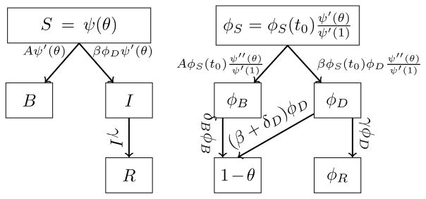
The flow diagram for disease spread with behavior change. Here A = (δBφB + δDφD).
In Figure 5, we show how behavior change modifies epidemic outcomes, using B to denote individuals whose behavior has changed. If the disease is introduced in a small number of individuals and behavior change spreads sufficiently faster than the disease, then the behavior change prevents the disease from having a large-scale epidemic.
FIG. 5.
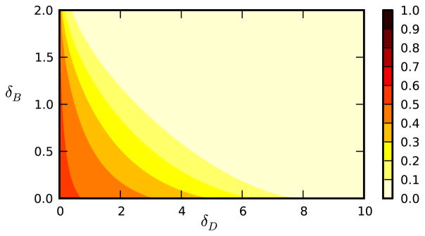
Computed final proportion infected for epidemics with behavior change. We use networks of the same structure as in Figure 3. The disease spreads with β = 2, γ = 1. The values of δB and δD are varied. For the initial condition, no individuals have changed behavior and a proportion 10−6 is initially infected randomly.
f. Summary
We have introduced an analytic model that calculates the simultaneous spread of two infectious diseases in a configuration model network. Our model is low dimensional regardless of the degree distribution. Using this model, we are able to calculate the effect of interactions between diseases in regimes that are inaccessible to analytic theories that do not include dynamics.
This model can easily be generalized to a range of other infectious processes. We have shown its application to behavior changes in response to a disease.
Supplementary Material
Acknowledgments
This work was supported by the RAPIDD program of the Science and Technology Directorate, Department of Homeland Security and the Fogarty International Center, National Institutes of Health (NIH), and by the Center for Communicable Disease Dynamics, Department of Epidemiology, Harvard School of Public Health under Award No. U54GM088558 from the National Institute Of General Medical Sciences (NIGMS). The content is solely the responsibility of the author and does not necessarily represent the official views of the NIGMS or the NIH.
References
- 1.Larremore D, Shew W, Restrepo J. Physical review letters. 2011;106:58101. doi: 10.1103/PhysRevLett.106.058101. [DOI] [PubMed] [Google Scholar]
- 2.Durrett R, Gleeson J, Lloyd A, Mucha P, Shi F, Sivakoff D, Socolar J, Varghese C. Proceedings of the National Academy of Sciences. 2012;109:3682. doi: 10.1073/pnas.1200709109. [DOI] [PMC free article] [PubMed] [Google Scholar]
- 3.Pastor-Satorras R, Vespignani A. Physical Review E. 2001;63:066117. doi: 10.1103/PhysRevE.63.066117. [DOI] [PubMed] [Google Scholar]
- 4.Funk S, Gilad E, Watkins C, Jansen V. Proceedings of the National Academy of Sciences. 2009;106:6872. doi: 10.1073/pnas.0810762106. [DOI] [PMC free article] [PubMed] [Google Scholar]
- 5.Bharathi S, Kempe D, Salek M. Internet and Network Economics. 2007;306 [Google Scholar]
- 6.Newman MEJ. Physical Review E. 2002;66:016128. [Google Scholar]
- 7.Pastor-Satorras R, Vespignani A. Physical Review Letters. 2001;86:3200. doi: 10.1103/PhysRevLett.86.3200. [DOI] [PubMed] [Google Scholar]
- 8.Boguñá M, Pastor-Satorras R, Vespignani A. Physical Review Letters. 2003;90:028701. doi: 10.1103/PhysRevLett.90.028701. [DOI] [PubMed] [Google Scholar]
- 9.May RM, Lloyd AL. Physical Review E. 2001;64:066112. doi: 10.1103/PhysRevE.64.066112. [DOI] [PubMed] [Google Scholar]
- 10.Miller JC. Physical Review E. 2007;76:010101(R). doi: 10.1103/PhysRevE.76.010101. [DOI] [PubMed] [Google Scholar]
- 11.Miller JC. Journal of Applied Probability. 2008;45:498. [Google Scholar]
- 12.Kenah E, Robins JM. Physical Review E. 2007;76:036113. doi: 10.1103/PhysRevE.76.036113. [DOI] [PMC free article] [PubMed] [Google Scholar]
- 13.Trapman P. Theoretical Population Biology. 2007;71:160. doi: 10.1016/j.tpb.2006.11.002. [DOI] [PubMed] [Google Scholar]
- 14.Volz EM, Meyers LA. Proceedings of the Royal Society B: Biological Sciences. 2007;274:2925. doi: 10.1098/rspb.2007.1159. [DOI] [PMC free article] [PubMed] [Google Scholar]
- 15.Miller JC, Slim AC, Volz EM. Journal of the Royal Society Interface. 2012;9:890. doi: 10.1098/rsif.2011.0403. [DOI] [PMC free article] [PubMed] [Google Scholar]
- 16.Miller JC, Volz EM. PloS One. 2013;8:e69162. doi: 10.1371/journal.pone.0069162. [DOI] [PMC free article] [PubMed] [Google Scholar]
- 17.Miller JC, Volz EM. Journal of Mathematical Biology. 2013;67:869. doi: 10.1007/s00285-012-0572-3. [DOI] [PMC free article] [PubMed] [Google Scholar]
- 18.Miller JC. Journal of The Royal Society Interface. 2009;6:1121. doi: 10.1098/rsif.2008.0524. [DOI] [PMC free article] [PubMed] [Google Scholar]
- 19.Miller JC. Physical Review E. 2009;80:020901(R). doi: 10.1103/PhysRevE.80.020901. [DOI] [PubMed] [Google Scholar]
- 20.Newman MEJ. Physical Review Letters. 2009;103:58701. doi: 10.1103/PhysRevLett.103.058701. [DOI] [PubMed] [Google Scholar]
- 21.Gleeson J, Melnik S, Hackett A. Physical Review E. 2010;81:066114. doi: 10.1103/PhysRevE.81.066114. [DOI] [PubMed] [Google Scholar]
- 22.Melnik S, Hackett A, Porter M, Mucha P, Gleeson J. Physical Review E. 2011;83:036112. doi: 10.1103/PhysRevE.83.036112. [DOI] [PubMed] [Google Scholar]
- 23.Volz EM, Miller JC, Galvani A, Meyers LA. PLoS Comput Biol. 2011;7:e1002042. doi: 10.1371/journal.pcbi.1002042. [DOI] [PMC free article] [PubMed] [Google Scholar]
- 24.House T, Keeling M. Journal of The Royal Society Interface. 2011;8:67. doi: 10.1098/rsif.2010.0179. [DOI] [PMC free article] [PubMed] [Google Scholar]
- 25.Eames KTD. Theoretical Population Biology. 2008;73:104. doi: 10.1016/j.tpb.2007.09.007. [DOI] [PubMed] [Google Scholar]
- 26.Andreasen V, Lin J, Levin S. Journal of mathematical biology. 1997;35:825. doi: 10.1007/s002850050079. [DOI] [PubMed] [Google Scholar]
- 27.Cobey S, Pascual M. Journal of Theoretical Biology. 2011;270:80. doi: 10.1016/j.jtbi.2010.11.009. [DOI] [PMC free article] [PubMed] [Google Scholar]
- 28.Eames K, Keeling M. Proceedings of the National Academy of Sciences. 2002;99:13330. doi: 10.1073/pnas.202244299. [DOI] [PMC free article] [PubMed] [Google Scholar]
- 29.Newman MEJ. Physical Review Letters. 2005;95:108701. doi: 10.1103/PhysRevLett.95.108701. [DOI] [PubMed] [Google Scholar]
- 30.Karrer B, Newman M. Physical Review E. 2011;84:036106. doi: 10.1103/PhysRevE.84.036106. [DOI] [PubMed] [Google Scholar]
- 31.Funk S, Jansen V. Physical Review E. 2010;81:036118. doi: 10.1103/PhysRevE.81.036118. [DOI] [PubMed] [Google Scholar]
- 32.Marceau V, Noël P, Hébert-Dufresne L, Allard A, Dubé L. Physical Review E. 2011;84:026105. doi: 10.1103/PhysRevE.84.026105. [DOI] [PubMed] [Google Scholar]
- 33.See Supplemental Material at [URL will be inserted by publisher] for more mathematical details of the derivations, regime analysis, and investigation of behavior change.
- 34.Newman MEJ. SIAM Review. 2003;45:167. [Google Scholar]
- 35.Molloy M, Reed B. Random Structures & Algorithms. 1995;6:161. [Google Scholar]
- 36.Karrer B, Newman MEJ. Physical Review E. 2010;82:016101. doi: 10.1103/PhysRevE.82.016101. [DOI] [PubMed] [Google Scholar]
- 37.A more complete explanation of a test individual can be found in the supplement and [40].
- 38.Decreusefond L, Dhersin JS, Moyal P, Tran VC. The Annals of Applied Probability. 2012;22:541. [Google Scholar]
- 39.A more detailed derivation of these boundaries is in the supplement.
- 40.Miller JC. Bulletin of Mathematical Biology. 2012;74:2125. doi: 10.1007/s11538-012-9749-6. [DOI] [PMC free article] [PubMed] [Google Scholar]
Associated Data
This section collects any data citations, data availability statements, or supplementary materials included in this article.