Optimized atomic statistical potentials: assessment of protein interfaces and loops

Abstract

Motivation: Statistical potentials have been widely used for modeling whole proteins and their parts (e.g. sidechains and loops) as well as interactions between proteins, nucleic acids and small molecules. Here, we formulate the statistical potentials entirely within a statistical framework, avoiding questionable statistical mechanical assumptions and approximations, including a definition of the reference state.

Results: We derive a general Bayesian framework for inferring statistically optimized atomic potentials (SOAP) in which the reference state is replaced with data-driven ‘recovery’ functions. Moreover, we restrain the relative orientation between two covalent bonds instead of a simple distance between two atoms, in an effort to capture orientation-dependent interactions such as hydrogen bonds. To demonstrate this general approach, we computed statistical potentials for protein–protein docking (SOAP-PP) and loop modeling (SOAP-Loop). For docking, a near-native model is within the top 10 scoring models in 40% of the PatchDock benchmark cases, compared with 23 and 27% for the state-of-the-art ZDOCK and FireDock scoring functions, respectively. Similarly, for modeling 12-residue loops in the PLOP benchmark, the average main-chain root mean square deviation of the best scored conformations by SOAP-Loop is 1.5 Å, close to the average root mean square deviation of the best sampled conformations (1.2 Å) and significantly better than that selected by Rosetta (2.1 Å), DFIRE (2.3 Å), DOPE (2.5 Å) and PLOP scoring functions (3.0 Å). Our Bayesian framework may also result in more accurate statistical potentials for additional modeling applications, thus affording better leverage of the experimentally determined protein structures.

Availability and implementation: SOAP-PP and SOAP-Loop are available as part of MODELLER (http://salilab.org/modeller).

Contact: sali@salilab.org

Supplementary information: Supplementary data are available at Bioinformatics online.

1 INTRODUCTION

Computational modeling can be used to predict the structures of whole proteins or their parts (e.g. loops and sidechains) as well as complexes involving proteins, peptides, nucleic acids and small molecules (Audie and Swanson, 2012; Baker and Sali, 2001; Dill and MacCallum, 2012; Ding et al., 2010; Skolnick et al., 2013; Wass et al., 2011). A modeling method requires a conformational sampling scheme for proposing alternative structures and a scoring function for ranking them. Significant progress has been made on both fronts (Fernández-Recio and Sternberg, 2010; Moult et al., 2011). In particular, many physics-based energy functions and statistical potentials computed from known protein structures have been described (Andrusier et al., 2007; Benkert et al., 2008; Betancourt and Skolnick, 2004; Betancourt and Thirumalai, 1999; Brenke et al., 2012; Chuang et al., 2008; Colovos and Yeates, 1993; Cossio et al., 2012; Dehouck et al., 2006; Fan et al., 2011; Ferrada et al., 2007; Gao and Skolnick, 2008; Gatchell et al., 2000; Hendlich et al., 1990; Huang and Zou, 2010; Jones, 1999; Keasar and Levitt, 2003; Kocher et al., 1994; Li et al., 2013; Liu and Gong, 2012; Liu and Vakser, 2011; Lu and Skolnick, 2001; Lu et al., 2008; McConkey et al., 2003; Melo and Feytmans, 1997; Melo et al., 2002; Miyazawa and Jernigan, 1996; Park and Levitt, 1996; Pierce and Weng, 2007; Qiu and Elber, 2005; Rajgaria et al., 2008; Rata et al., 2010; Reva et al., 1997; Rojnuckarin and Subramaniam, 1999; Rykunov and Fiser, 2010; Samudrala and Moult, 1998; Shapovalov and Dunbrack, 2011; Shen and Sali, 2006; Simons et al., 1997; Sippl, 1993; Summa et al., 2005; Tanaka and Scheraga, 1975; Wang et al., 2004; Xu et al., 2009; Zhang and Zhang, 2010; Zhao and Xu, 2012; Zhou and Skolnick, 2011; Zhou and Zhou, 2002; Zhu et al., 2008).

Derivation of a statistical potential has often been guided by an analogy between a sample of known native structures and the canonical ensemble in statistical mechanics, suggesting that the distributions of spatial features in the sample of native structures follow the Boltzmann distribution (Sippl, 1990). Thus, statistical potentials are generally calculated in two steps: (i) extracting a probability distribution of a spatial feature (e.g. a distance spanned by a specific pair of atom types) from a sample of known protein structures and (ii) normalizing this distribution by a reference distribution (e.g. the distribution of all distances, regardless of the atom types). Statistical potentials can differ in a number of aspects, including the sample of known protein structures, the protein representation (e.g. centroids of amino acid residues, C_α atoms and all atoms), the restrained spatial feature (e.g. solvent accessibility, distance, angles and orientation between two sets of atoms), the sequence features (e.g. amino acid residue types, atom types, residue separation in sequence and chain separation), the treatment of sparse samples and the definition of the reference state. Here, we optimize the accuracy of a statistical potential over most of these aspects. This optimization challenge is addressed by formulating a statistical potential independently from any assumptions grounded in statistical mechanics; instead, we rely on a Bayesian approach based on data alone. Although the proposed theory applies to any kind of a statistical potential, we illustrate it by deriving specific statistical potentials for protein–protein docking and loop modeling.

2 METHOD

We begin by defining statistical potentials in terms of distributions extracted from known protein structures (Section 2.1), followed by a description of a protocol to actually compute a statistical potential (Sections 2.2–2.7, Fig. 1).

Fig. 1.

Flowchart for optimizing statistical potentials. The corresponding sections in the text are indicated

2.1 Theory

For structure characterization of a given protein sequence by either experiment or theory, we ideally need a joint probability density function (pdf) for the structure, given everything we know about it (Shen and Sali, 2006). In general, our knowledge can come from different kinds of experiments with the protein (e.g. X-ray crystallography), physical theories (e.g. a molecular mechanics force field) and/or statistical inference (e.g. all known structures or only homologous known structures). Here, we focus on a joint pdf for a given sequence based on the knowledge of all known protein structures deposited in the Protein Data Bank (PDB) (Kouranov et al., 2006); thus, our joint pdf is a statistical potential.

To derive the joint pdf for a structure of a sequence, we need to approximate it by using terms that can actually be computed from the PDB. The structure X of an amino acid sequence is defined by the set of its features , such as a distance between two specific atoms. Thus, we can approximate the joint pdf by the product of pdfs (restraints) for individual features:

(1)

Without any loss of accuracy, we define the restraint as the ratio between the feature distribution from a sample of informative features in a set of proteins with known structures (e.g. for a distance, all distances spanned by the same atom types in ) and an unknown recovery function :

(2)

In other words, the recovery function is defined such that the product of restraints approximates the joint pdf as well as possible (c.f., Equation 1), while minimizing the number of parameters that need to be fit to the data. Construction of the sample of informative features involves a compromise between including only features of known structures that are most likely to resemble the predicted feature (which minimizes sample size) and minimizing the statistical noise (which maximizes sample size). The features used in the sample are termed to be of the same type as the inferred feature (Section 2.2). The restraints on all features of of type are calculated from the same set of informative features and thus are the same. Here, the sample of informative features includes all features of the same type from representative known protein structures (Section 2.3).

2.2 Feature types

To illustrate the general theory mentioned earlier in the text, we derive optimized statistical potentials for assessing protein–protein interfaces (SOAP-PP) and loop conformations (SOAP-Loop). We restrain the following feature types:

2.2.1 Atomic distance

Distance is considered to depend on atom types and as well as the ‘covalent separation’ between the two atoms (). The atom type depends on the residue type, resulting in the total of 158 atoms types for the 20 standard residue types (Shen and Sali, 2006). Covalent separation is measured in three ways. First, by the minimum number of covalent bonds between the two atoms (bond separation). Second, by the number of residues separating the two atoms in the polypeptide chain (residue separation). Third, by chain separation, which is 0 if the atoms are in the same chain and 1 otherwise. The distance is mapped in the range from 0 to a parameterized distance cutoff, such as 15 Å.

2.2.2 Orientation between a pair of covalent bonds

Orientation is defined by a distance , two angles and a dihedral angle (Fig. 2). It is considered to depend on covalent bond types () defined in turn by their atom types and covalent separation (); there are 316 covalent bond types for the 20 standard residue types.

Fig. 2.

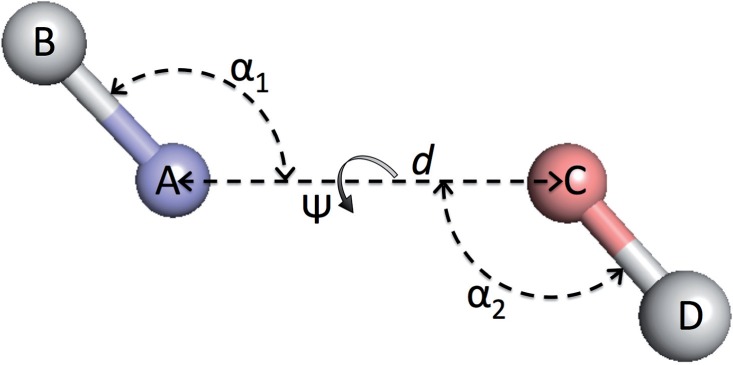
Distance and angles between two covalent bonds, A–B and C–D. , distance between atoms A and C. , angle between atoms B, A and C. , angle between atoms A, C and D. , dihedral angle between atoms B, A, C and D. is defined using atoms A and C

2.2.3 Relative atomic surface accessibility

Accessibility is considered to depend on the atom type () (Sali and Blundell, 1993).

2.3 Feature distributions

2.3.1 Known protein structures

A small fraction of the known protein structures from the PDB (and their decoy structures) is used only for assessing the accuracy of statistical potentials (Section 2.5). The remaining structures from the PDB are filtered to construct the known protein structure set , including only structures determined by X-ray crystallography at the resolution better than 2.2 Å and R_free better than 25%. Three additional subsets of representative structures were obtained by requiring at most 30, 60 and 95% sequence identity to any other representative structure, respectively, with preference for structures determined at higher resolutions and with lower R_free values. A statistical potential is optimized by choosing among the entire set or its three subsets to estimate the feature distributions .

2.3.2 Calculation of feature distributions

The sample for computing this distribution is the set of the individual features of type in protein set , where each feature is represented by the distribution of this feature -. The feature distribution is the average of these sample distributions. For a distance and an angle, is approximated by a Gaussian distribution with the mean equal to the observed value and the standard deviation computed by the propagation (Neuhauser, 2010) of the uncertainties of individual atomic positions, which in turn are estimated from the atomic isotropic temperature factors (Carugo and Argos, 1999; Cruickshank, 1999; Schneider, 2000). For relative atomic surface accessibility, is approximated using a delta function centered at feature in . The approximated feature distribution is then computed from the approximated sample distributions .

2.4 Bayesian smoothing and smoothing priors

The feature distributions can be noisy when the sample is relatively small, as is often the case for the orientation between a pair of covalent bonds (Fig. 3A). Thus, we use Bayesian inference to calculate a smooth feature distribution:

(3)

where is the ideal distribution without noise from an infinitely large set of known structures. Both the likelihood and the prior are multivariate Gaussian distributions (Rasmussen and Williams, 2005). The smoothness of is specified by the prior ; here, the prior is a multivariate Gaussian distribution with a zero mean and a squared exponential covariance function (Mackay, 2003). The characteristic length scale of the covariance function defines the range over which the two points are still correlated (the smoothness of the curve). We set the characteristic length equal to a scale parameter multiplied by 0.2 Å for distance, 10° for angles and 0.1% for atomic surface accessibility. A set of smoothing priors is obtained by varying . Using a scale of 2.0 as an example, the inferred is significantly smoother than (Fig. 3B).

Fig. 3.

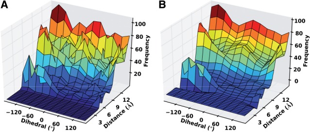
Distance and dihedral angle joint distribution between alanine N-C_α and alanine O-C, when and . (A) Original distribution. (B) Smoothed distribution

2.5 Decoys and assessment criteria

2.5.1 Learning set for SOAP-PP

This set consists of 176 native complex structures in the pairwise protein docking benchmark 4.0 (Hwang et al., 2010) and ∼4500 decoys for each of the complexes generated using PatchDock (Duhovny et al., 2002).

2.5.2 Testing set for SOAP-PP

This set consists of 176 native complex structures in the pairwise protein docking benchmark 4.0 (Hwang et al., 2010) as well as ∼212 000 decoys for each of the complexes generated using PatchDock (Duhovny et al., 2002) and ∼54 000 decoys for each of the complexes generated using ZDOCK (Pierce et al., 2011).

2.5.3 Assessment criteria for SOAP-PP

Each model is assessed for accuracy based on root mean square deviation (RMSD) from the native structure, as used at CAPRI (Lensink et al., 2007). A docking model is considered acceptable if the ligand C_α RMSD after superposition of the receptors is <10 Å or the interface C_α RMSD is <4 Å. A docking model is of medium accuracy if ligand C_α RMSD is <5 Å or interface C_α RMSD is <2 Å. The success rate for SOAP-PP is the percentage of benchmark cases with at least one medium or acceptable accuracy model in the top N predictions.

2.5.4 Learning set for SOAP-Loop

This set consists of 3838 native loop conformations of 4–20 residues and ∼500 decoys for each loop generated using MODELLER (Fiser and Sali, 2003; Sali and Blundell, 1993). Loops were extracted from X-ray crystallography structures in the PDB using DSSP (Kabsch and Sander, 1983; Joosten et al., 2011). We only considered protein structures determined at a resolution better than 2 Å, R_free better than 0.25 and crystallized between pHs 6.5 and 7.5; no pair of source structures had sequence identity higher than 30%. Each loop has only standard residues, no missing non-hydrogen atoms, average atomic surface accessibility between 5 and 60%, no crystal contacts, no clashes with nearby atoms, no contacts with metal ligands and does not occur in the PLOP loop modeling decoy set (Jacobson et al., 2004).

2.5.5 Testing set for SOAP-Loop

This set consists of 833 native loop conformations of 4–12 residues and ∼450 decoys for each loop generated using PLOP (Jacobson et al., 2004).

2.5.6 Assessment criteria for SOAP-Loop

Each model is assessed for accuracy based on its main-chain RMSD to the native conformation, after superposition of all non-loop atoms (RMSD_global) (Fiser et al., 2000); main-chain atoms include amide nitrogen, C_α, as well as carbonyl carbon and oxygen. SOAP-Loop is assessed by the average RMSD_global of the top ranked model for each loop.

2.6 Recovery functions and functional forms

We estimate the recovery function by optimizing the accuracy of the corresponding statistical potential on a benchmark of interest. To avoid overfitting, we assume either a single recovery function for all feature types or the same recovery function for a subset of similarly distributed feature types.

The set of recovery function forms is different for distances, angles and accessibility: The recovery function for the atomic distance is modeled using one of three functional forms: (i) , where d is distance and q is a constant (Zhou and Zhou, 2002); (ii) the ideal gas distribution in spheres with varying radii (Shen and Sali, 2006); and (iii) spliced cubic splines. For orientation, the recovery function is defined as the product of a recovery function for , , and respectively. The recovery functions for angles , and dihedral angle are modeled using two different functional forms: (i) the feature distribution calculated using the ideal gas assumption and (ii) spliced cubic splines. For the relative atomic surface accessibility, the recovery function form is spliced cubic splines. Control points of cubic splines are defined by their x and y values. When searching for the best cubic spline recovery function, the x values of the control points are either fixed at discrete sampling values or inferred together with the y values.

To optimize the recovery functions, we need to balance minimizing noise and maximizing precision. Thus, for atomic distances, we clustered the distance distributions for different atom type pairs using k-mean clustering and assumed that the pairs of atom types with similar distance distributions have a similar recovery function (Fig. 4).

Fig. 4.

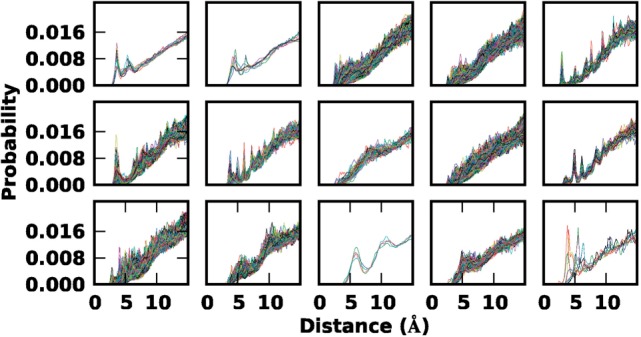
Distance distributions for different atom pairs are clustered into 15 different groups. Each line represents a distance distribution from a pair of atoms of certain types. Each group has 6–8401 distributions. During k-mean clustering, the number of clusters was set to 20, resulting in 14 clusters with >5 distributions and 6 clusters with <5 distributions; the latter 6 clusters are grouped together (bottom right panel)

2.7 Bayesian inference and model selection

A statistical potential is defined by four discrete input variables (the known protein structure subset , the feature type subset , the smoothing prior and the recovery function form ) and a vector of continuous input variables (the recovery function parameters ). We elected to define the best values for the four discrete variables are those that result in the most generalizable statistical potential, as judged by the Bayesian predictive densities (Vehtari and Lampinen, 2002), whereas the best values for the recovery function parameters are those that result in the most accurate statistical potential, as judged by a given benchmark. Because each of the five variables can be sampled at many values, enumeration of all combinations is not computationally feasible. Thus, the search for the best values is carried out in four stages, as follows.

First, irrespective of the final restrained feature , we begin with the atomic distance and a single recovery function for all atom type pairs. The optimal values of the discrete variables are found by an iterative discrete search:

1. Choose an arbitrary starting value for each variable out of their possible value sets (Supplementary Table S1 and S2).

2. For each variable, choose the best value and eliminate the worst value in the value set using Bayesian model selection based on Bayesian predictive densities (Vehtari and Lampinen, 2002). The Bayesian predictive density for each value is calculated with other variables fixed at their best previous values:

   (4)

   where the learning decoys D are randomly separated multiple times into a training set and a validation set , from which the integrals are estimated using Monte Carlo sampling (Evans and Swartz, 2000). is calculated following the Bayes rule:

   (5)

   here the likelihood is a half-normal distribution whose corresponding normal distribution has the mean equal to the accuracy of an imaginary statistical potential generating scores that correlate perfectly with the decoy-native RMSD and the standard deviation computed by dividing the mean by the number of the cases in the training set ; the prior is an informative prior defining a reasonable range for .

3. Repeat step 2 until the best values do not change.

4. Repeat five times steps 1–3 for different random initial values.

5. Keep the best performing variable values.

Second, keeping the optimal values from the previous step fixed, we find the optimal values for the feature type, smoothing length scale and the number of spline anchor points using the same 5-step iterative discrete search outlined earlier in the text.

Third, if the optimal spatial feature selected in the previous step is not orientation, we vary the number of recovery functions and the number of anchor points to optimize their values, again using the 5-step iterative discrete search.

Fourth, using the selected , we infer the best recovery function parameter values by maximizing (Equation 5). The optimized statistical potential is then calculated (Equation 2) and assessed on testing decoy sets.

SOAP-PP and SOAP-Loop are available as part of MODELLER (http://salilab.org/modeller). All the training, learning, testing, decoys, benchmark sets and scripts are available at http://salilab.org/SOAP.

3 RESULTS

3.1 Scoring protein–protein interfaces

SOAP-PP is an atomic statistical potential for assessing a binary protein interface, computed with our Bayesian framework by optimizing its accuracy on the learning set for SOAP-PP (Supplementary Table S1).

Using the recovery function parameters optimized for 15 sets of training decoys (each set is randomly selected 50% of the learning set), the average top10 success rate (Section 2.5.3) is 44.7 ± 1.2% on the sets of training decoys and 38.4 ± 1.7% on the sets of validation decoys. The relatively small difference between the two success rates likely results from overfitting. To investigate overfitting, we increased the size of the training decoy set from 50 to 67% of the entire learning set of 176 proteins. As a result, the average top10 success rate on the training decoys decreased from 44.7 to 44.2%, but the average success rate on the validation decoys (the remaining 33% of the learning set) increased from 38.4 to 39.8%. This observation suggested that increasing the size of the training set may be an effective way of reducing overfitting (Murphy, 2012). Thus, we optimized SOAP-PP using the entire learning set of 176 proteins as the training set, even though this forces subsequent testing on the training protein sequences. To estimate the resulting overfitting, we calculated six optimized statistical potentials, each one of which was based on a training set that included a random subset of ∼67% of the learning set. Next, we tested these potentials on two testing sets: the first set consisted only of the training proteins; the second set consisted of the remaining learning proteins. The average top10 success rate for the PatchDock decoys is 41.1% and 38.6% for the first and second test set, respectively; for the ZDOCK decoys, the average top10 success rate is 40.0 and 38.9% for the first and second test set, respectively. Therefore, given that increasing the training set size reduces overfitting as shown previously, the accuracy of SOAP-PP estimated based on a completely different testing set is expected to be within 2.5% of the current estimate (later in the text).

SOAP-PP was assessed on the PatchDock (Schneidman-Duhovny et al., 2012) and ZDOCK decoy sets (Pierce et al., 2011) (Fig. 5). For PatchDock decoys, the top10 success rate of SOAP-PP is 40% (Fig. 5A) compared with 23% for ZRANK and 27% for FireDock. If only models of medium or better accuracy are considered, the top10 success rate is 33% for SOAP, 17% for ZRANK and 23% for FireDock (Fig. 5B). For ZDOCK decoys, the top10 success rate of SOAP-PP is 41% (Fig. 5C) compared with 30% for ZRANK and 22% for FireDock. If only models of medium or better accuracy are considered, the success rate is 32% for SOAP-PP, 22% for ZRANK and 17% for FireDock (Fig. 5D).

Fig. 5.

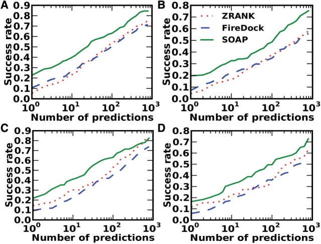
Success rates of SOAP-PP, ZRANK and FireDock on the PatchDock and ZDOCK decoy sets. (A) Success rates on the PatchDock decoy set, where a success is defined as having an acceptable accuracy structure in the top N predictions (x-axis). (B) Success rates on the PatchDock decoy set for picking structures with medium accuracy. (C) Success rates on the ZDOCK decoy set for picking structures with acceptable accuracy. (D) Success rates on the ZDOCK decoy set for picking structures with medium accuracy

High accuracy of SOAP-PP can sometimes be attributed to the weaker short-distance repulsion (Fig. 6A) compared with ZRANK (Pierce and Weng, 2007) and FireDock (Andrusier et al., 2007), both of which use a modified van der Waals repulsion term; thus, the clashes of the best sampled structure with a receptor are likely less penalized by SOAP than by ZRANK and FireDock. Although SOAP-PP is more successful than ZRANK and FireDock overall, picking near-native protein–protein complex models out of decoys remains a hard problem (Fig. 5). For some cases, all three scoring functions perform badly, especially when the protein–protein interfaces are small and have poor shape complementarity (Fig. 6B).

Fig. 6.

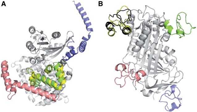
Comparison of the top ranked, best sampled and native configurations. (A) 2G77. (B) 1OC0. The receptor is shown in gray. The ligand is shown in the native configuration (yellow), the best sampled configuration (green for 2G77 and black for 1OC0) and the top ranked configuration by SOAP (green), FireDock (blue) and ZRANK (red)

3.2 Scoring loops

SOAP-Loop is an atomic statistical potential for assessing protein loop conformations, computed with our Bayesian framework by optimizing its accuracy on the learning set for SOAP-Loop (Supplementary Table S2).

SOAP-Loop was assessed on the PLOP loop modeling decoy set (Jacobson et al., 2004). We compare SOAP-Loop with DOPE (Shen and Sali, 2006), DFIRE (Zhang et al., 2004), Rosetta 3.3 (Simons et al., 1999) and PLOP 25.6 scoring functions (Jacobson et al., 2004) (Fig. 7A). For short loops, SOAP-Loop and Rosetta perform similarly and better than the other tested scoring functions: the main-chain RMSD of SOAP-Loop’s top ranked structure is close to that of the best decoy structure. For longer loops, the accuracy differences become larger. SOAP-Loop is still able to pick structures close to the best decoy structures: for 12-residue loops, the average main-chain RMSD of the best scored conformations by SOAP-Loop is 1.5 Å, close to the average RMSD of the best decoy conformations (1.2 Å) and significantly better than that by DOPE (2.5 Å), DFIRE (2.3 Å), Rosetta (2.1 Å) and PLOP scoring functions (3.0 Å). We note that this assessment should not be used to rank the PLOP scoring function because the decoy set used here was generated with PLOP. Thus, we further compare different scoring functions by their average all-atom RMSD values of the best scored conformations using our learning set for SOAP-Loop (Section 2.5.4 and Supplementary Table S3).

Fig. 7.

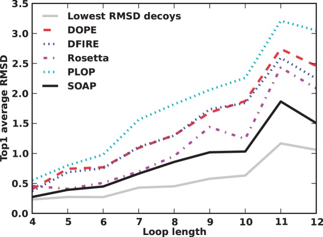
Accuracy of SOAP-Loop. The average main-chain RMSD of top ranked structures by DOPE, DFIRE, Rosetta, PLOP and SOAP-Loop on PLOP loop modeling decoys. The average RMSD of the most accurate conformations sampled by PLOP is plotted by a dash-dotted line

Although no testing protein occurs in the learning set, 11 pairs of testing-learning loops have the same sequence. Excluding these 11 loops from the testing set, the average RMSD of the top ranked loop by SOAP-Loop increases insignificantly from 0.895 Å to 0.897 Å; the average RMSD of the best decoy conformations also increases insignificantly from 0.566 Å to 0.567 Å.

The relative success of SOAP is attributed to the scoring of the orientation instead of distance and the use of the recovery functions instead of a reference state (Fig. 8). However, SOAP-Loop still fails to identify the best-sampled conformation in some cases. For a loop in 1CYO, for example, the failure can be attributed to the lack of a sufficiently native conformation among the tested conformations and the absence of significant interactions between the loop and the rest of the protein (Fig. 9A). It is also possible that some interactions, such as long-range interactions, are not treated accurately by any scoring function, indicating the need for further development of the theory of statistical potentials.

Fig. 8.

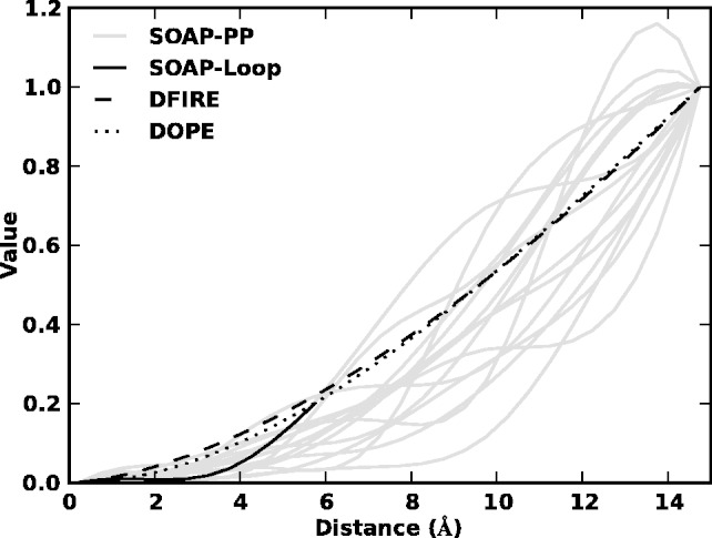
Recovery functions for SOAP-PP and SOAP-Loop are compared with DOPE and DFIRE’s reference states

Fig. 9.

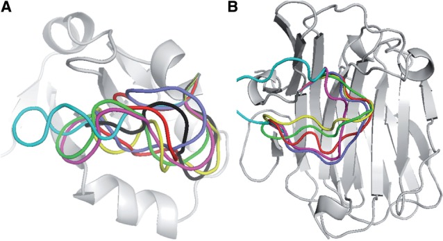
Comparison of the top ranked, best sampled and native configurations. (A) 1CYO. (B) 2AYH. The native structure is shown in light gray. The loop is shown in the native configuration (yellow), the best sampled configuration (black for 1CYO and green for 2AYH) and the top ranked configuration by SOAP (green), DOPE (blue), DFIRE (red), Rosetta (magenta) and PLOP (light blue)

4 DISCUSSION

We developed a Bayesian approach to optimizing statistical potentials based on probability theory and without recourse to questionable statistical mechanical assumptions and approximations. We also applied this approach to calculate optimized statistical potentials for assessing protein interactions (SOAP-PP) and loops (SOAP-Loop). These two statistical potentials perform better than others in their class. For PatchDock and ZDOCK decoys, the top10 success rate of SOAP-PP is >10% higher than that of FireDock and ZRANK (Fig. 5). For 12-residue loops in the PLOP benchmark, the average main-chain RMSD of the best scored conformations by SOAP-Loop is 1.5 Å, close to the average RMSD of the best sampled conformations (1.2 Å) and significantly better than that from DOPE (2.5 Å), DFIRE (2.3 Å), Rosetta (2.1 Å) and PLOP scoring functions (3.0 Å) (Fig. 7). The relative accuracy of SOAP-PP and SOAP-Loop results primarily from normalizing the raw distributions by the recovery functions instead of a reference state, restraining of orientation instead of only distance and thoroughly optimizing parameter values while avoiding overfitting.

Next, we discuss three points in turn. First, we describe our recovery functions and compare them with the reference states used for other statistical potentials. Second, we discuss the importance of restraining orientation and using covalent separation as an independent variable. Finally, we conclude by commenting on future improvements of our Bayesian approach and its applications.

4.1 Cubic splines as a recovery function form

A key difference between statistical potentials is the definition of their reference states, which are often derived by assuming that the PDB provides a Boltzmann ensemble of structural features (Sippl, 1990). Here, we replace the reference state by data-driven recovery functions, defined self-consistently without recourse to these questionable statistical mechanical assumptions (Finkelstein et al., 1995; Shen and Sali, 2006). In an extreme case, we use cubic splines to compute optimal recovery functions, relying on Bayesian inference to obtain parameter values that result in the most accurate statistical potential given a benchmark.

The use of splines as recovery functions is motivated by a qualitative analysis of the recovery function (Supplementary Equation S2). The distribution of a single feature is the product of the restraint on and an integral involving the restraints on ’s other features (i.e. the environment restraint). Then, the recovery function is the distribution of feature type in structure set resulting from the environmental restraints alone (Supplementary Equation S2). We now discuss three implications of this perspective.

First, if we assume that atoms are placed randomly within the protein shell, a recovery function will be similar to the DFIRE and DOPE reference states based on the ideal gas assumption (Shen and Sali, 2006; Zhou and Zhou, 2002).

Second, using the distance d between atoms A and C in Figure 2 as an example, the environment restraint on d is a consequence of the restraints on distances between A–D, C–B and B–D as well as the bonds between A–B and C–D. The restraints on A–D, C–B and B–D distances have short-range repulsion components. Thus, the environment restraint on the distance A–C will include an effective short-range repulsion. This qualitative analysis is consistent with the observed recovery functions for SOAP-PP and SOAP-Loop, which all have lower values at short distances than the DOPE reference state based on the ideal gas assumption (Fig. 8).

Finally, the recovery functions for different feature types can vary, because of their different environments, as observed for the recovery functions for 15 clusters of atom type pairs used in SOAP-PP (Fig. 8).

Although splines can mimic almost any smooth function given a sufficient number of anchor points, its flexibility could also lead to overfitting; moreover, a large number of anchor points could lead to oscillations (Fig. 8). Although our Bayesian model selection method helps with the generalizability of the optimized cubic spline (Vehtari and Lampinen, 2002), it is conceivable that applying Bayesian model selection to a less flexible but appropriate functional form will result in a more accurate and general statistical potential than that based on splines.

4.2 Spatial and sequence features

Our orientation restraints score a spatial relationship between two sets of atoms in more detail than distance restraints alone, and should be particularly useful for scoring spatial relationships between polar atoms, especially for hydrogen bond donors and acceptors. In fact, the relative accuracy of SOAP-Loop can be attributed to the use of orientation and recovery functions instead of distance and reference state, respectively (Supplementary Table S1). However, using orientation did not result in a better statistical potential for ranking protein interfaces (Supplementary Table S2). Although we may not have found the globally optimal statistical potential for orientation, a more likely reason is insufficient accuracy of the tested conformations produced by rigid docking.

Covalent separation is another important factor affecting the accuracy of the derived statistical potentials. Surprisingly, for ranking protein interfaces, statistical potentials derived from intra-chain non-local atom pairs (bond separation >9) work better than statistical potentials derived from inter-chain atom pairs (chain separation = 1) (Supplementary Table S1). A likely reason is that many protein interfaces in the PDB result from crystal contacts that do not reflect interfaces between proteins in solution (Carugo and Argos, 1997; Krissinel, 2010). In the future, a better statistical potential for ranking protein interfaces might be obtained if only true biological interfaces from PDB are used.

4.3 Bayesian inference

Statistical potentials can be derived for many different values of the input variables, with little or no a priori reasons to choose one set of values over the others. The Bayesian model selection based on Bayesian predictive densities provides a statistically rigorous way of choosing the values that result in most generalizable statistical potentials (Vehtari and Lampinen, 2002). However, one limitation of this method is that the calculation of predictive densities is computational intensive, often requiring more than tens of thousands of evaluations of the statistical potential on the benchmark. Thus, such calculations are not always practical. Fortunately, increases in the available computer power will enable us to find more accurate statistical potentials in an increasingly larger parameter space in the future. Another approach to improving the search for optimal parameter values is to use physically motivated feature types, functional forms and allowed value ranges.

In principle, normalizing the feature distributions by recovery functions to obtain a statistical potential (Equation 2) is not necessary. Instead, we could use parametric (e.g. the mathematical functional forms used in molecular mechanics force fields) or non-parametric functions to represent the statistical potential and directly infer the optimal statistical potential by its accuracy on a benchmark of interest. However, this approach might not provide an accurate statistical potential in practice because of the large number of parameters whose values would need to be optimized.

Our method for smoothing feature distributions is a generalization of the two related methods used in calculating statistical potentials (Sippl, 1990) and homology restraints (Sali and Blundell, 1993). Both methods are equivalent to our Bayesian smoothing method with a diagonal covariance matrix as the smoothing prior. Their prior distribution is equivalent to the mean of our prior , whereas the weights on their prior distributions are defined by the standard deviation in our covariance matrix.

In conclusion, our Bayesian framework can be applied to derive an optimized statistical potential for many other kinds of modeling problems for which sample structures are available, thus affording better leverage of the experimentally determined protein structures. Examples include membrane protein topology and complexes of proteins with small molecules or peptides.

Funding: NIH grants (GM071790 and GM093342; R01 GM054762 to A.S.).

Conflicts of Interest: none declared.

REFERENCES

- Andrusier N, et al. FireDock: fast interaction refinement in molecular docking. Proteins. 2007;69:139–159. doi: 10.1002/prot.21495. [DOI] [PubMed] [Google Scholar]
- Audie J, Swanson J. Recent work in the development and application of protein-peptide docking. Future Med. Chem. 2012;4:1619–1644. doi: 10.4155/fmc.12.99. [DOI] [PubMed] [Google Scholar]
- Baker D, Sali A. Protein structure prediction and structural genomics. Science. 2001;294:93–96. doi: 10.1126/science.1065659. [DOI] [PubMed] [Google Scholar]
- Benkert P, et al. QMEAN: a comprehensive scoring function for model quality assessment. Proteins. 2008;71:261–277. doi: 10.1002/prot.21715. [DOI] [PubMed] [Google Scholar]
- Betancourt MR, Thirumalai D. Pair potentials for protein folding: choice of reference states and sensitivity of predicted native states to variations in the interaction schemes. Protein Sci. 1999;8:361–369. doi: 10.1110/ps.8.2.361. [DOI] [PMC free article] [PubMed] [Google Scholar]
- Betancourt MR, Skolnick J. Local propensities and statistical potentials of backbone dihedral angles in proteins. J. Mol. Biol. 2004;342:635–649. doi: 10.1016/j.jmb.2004.06.091. [DOI] [PubMed] [Google Scholar]
- Brenke R, et al. Application of asymmetric statistical potentials to antibody-protein docking. Bioinformatics. 2012;28:2608–2614. doi: 10.1093/bioinformatics/bts493. [DOI] [PMC free article] [PubMed] [Google Scholar]
- Carugo O, Argos P. Protein-protein crystal-packing contacts. Protein Sci. 1997;6:2261–2263. doi: 10.1002/pro.5560061021. [DOI] [PMC free article] [PubMed] [Google Scholar]
- Carugo O, Argos P. Reliability of atomic displacement parameters in protein crystal structures. Acta Crystallogr. D Biol. Crystallogr. 1999;55:473–478. doi: 10.1107/s0907444998011688. [DOI] [PubMed] [Google Scholar]
- Chuang G-Y, et al. DARS (Decoys As the Reference State) potentials for protein-protein docking. Biophys. J. 2008;95:4217–4227. doi: 10.1529/biophysj.108.135814. [DOI] [PMC free article] [PubMed] [Google Scholar]
- Colovos C, Yeates TO. Verification of protein structures: patterns of nonbonded atomic interactions. Protein Sci. 1993;2:1511–1519. doi: 10.1002/pro.5560020916. [DOI] [PMC free article] [PubMed] [Google Scholar]
- Cossio P, et al. A simple and efficient statistical potential for scoring ensembles of protein structures. Sci. Rep. 2012;2:351. [Google Scholar]
- Cruickshank DW. Remarks about protein structure precision. Acta Crystallogr. D Biol. Crystallogr. 1999;55:583–601. doi: 10.1107/s0907444998012645. [DOI] [PubMed] [Google Scholar]
- Dehouck Y, et al. A new generation of statistical potentials for proteins. Biophys. J. 2006;90:4010–4017. doi: 10.1529/biophysj.105.079434. [DOI] [PMC free article] [PubMed] [Google Scholar]
- Dill KA, MacCallum JL. The protein-folding problem, 50 years on. Science. 2012;338:1042–1046. doi: 10.1126/science.1219021. [DOI] [PubMed] [Google Scholar]
- Ding X-M, et al. Computational prediction of DNA-protein interactions: a review. Curr. Comput. Aided Drug Des. 2010;6:197–206. doi: 10.2174/157340910791760091. [DOI] [PubMed] [Google Scholar]
- Duhovny D, et al. Second International Workshop, WABI 2002. 2002. Efficient Unbound Docking of Rigid Molecules; pp. 185–200. [Google Scholar]
- Evans M, Swartz T. Approximating Integrals Via Monte Carlo and Deterministic Methods. New York, USA: Oxford University Press; 2000. [Google Scholar]
- Fan H, et al. Statistical potential for modeling and ranking of protein-ligand interactions. J. Chem. Inf. Model. 2011;51:3078–3092. doi: 10.1021/ci200377u. [DOI] [PMC free article] [PubMed] [Google Scholar]
- Fernández-Recio J, Sternberg MJE. The 4th meeting on the Critical Assessment of Predicted Interaction (CAPRI) held at the Mare Nostrum, Barcelona. Proteins Struct. Funct. Bioinform. 2010;78:3065–3066. [PubMed] [Google Scholar]
- Ferrada E, et al. A knowledge-based potential with an accurate description of local interactions improves discrimination between native and near-native protein conformations. Cell Biochem. Biophys. 2007;49:111–124. doi: 10.1007/s12013-007-0050-5. [DOI] [PubMed] [Google Scholar]
- Finkelstein AV, et al. Why do protein architectures have Boltzmann-like statistics? Proteins. 1995;23:142–150. doi: 10.1002/prot.340230204. [DOI] [PubMed] [Google Scholar]
- Fiser A, et al. Modeling of loops in protein structures. Protein Sci. 2000;9:1753–1773. doi: 10.1110/ps.9.9.1753. [DOI] [PMC free article] [PubMed] [Google Scholar]
- Fiser A, Sali A. ModLoop: automated modeling of loops in protein structures. Bioinformatics. 2003;19:2500–2501. doi: 10.1093/bioinformatics/btg362. [DOI] [PubMed] [Google Scholar]
- Gao M, Skolnick J. DBD-Hunter: a knowledge-based method for the prediction of DNA-protein interactions. Nucleic Acids Res. 2008;36:3978–3992. doi: 10.1093/nar/gkn332. [DOI] [PMC free article] [PubMed] [Google Scholar]
- Gatchell DW, et al. Discrimination of near-native protein structures from misfolded models by empirical free energy functions. Proteins. 2000;41:518–534. [PubMed] [Google Scholar]
- Hendlich M, et al. Identification of native protein folds amongst a large number of incorrect models. The calculation of low energy conformations from potentials of mean force. J. Mol. Biol. 1990;216:167–180. doi: 10.1016/S0022-2836(05)80068-3. [DOI] [PubMed] [Google Scholar]
- Huang S-Y, Zou X. Inclusion of solvation and entropy in the knowledge-based scoring function for protein-ligand interactions. J. Chem. Inf. Model. 2010;50:262–273. doi: 10.1021/ci9002987. [DOI] [PMC free article] [PubMed] [Google Scholar]
- Hwang H, et al. Performance of ZDOCK and ZRANK in CAPRI rounds 13-19. Proteins. 2010;78:3104–3110. doi: 10.1002/prot.22764. [DOI] [PMC free article] [PubMed] [Google Scholar]
- Jacobson MP, et al. A hierarchical approach to all-atom protein loop prediction. Proteins. 2004;55:351–367. doi: 10.1002/prot.10613. [DOI] [PubMed] [Google Scholar]
- Jones DT. GenTHREADER: an efficient and reliable protein fold recognition method for genomic sequences. J. Mol. Biol. 1999;287:797–815. doi: 10.1006/jmbi.1999.2583. [DOI] [PubMed] [Google Scholar]
- Joosten RP, et al. A series of PDB related databases for everyday needs. Nucleic Acids Res. 2011;39:D411–D419. doi: 10.1093/nar/gkq1105. [DOI] [PMC free article] [PubMed] [Google Scholar]
- Kabsch W, Sander C. Dictionary of protein secondary structure: pattern recognition of hydrogen-bonded and geometrical features. Biopolymers. 1983;22:2577–2637. doi: 10.1002/bip.360221211. [DOI] [PubMed] [Google Scholar]
- Keasar C, Levitt M. A novel approach to decoy set generation: designing a physical energy function having local minima with native structure characteristics. J. Mol. Biol. 2003;329:159–174. doi: 10.1016/S0022-2836(03)00323-1. [DOI] [PMC free article] [PubMed] [Google Scholar]
- Kocher JP, et al. Factors influencing the ability of knowledge-based potentials to identify native sequence-structure matches. J. Mol. Biol. 1994;235:1598–1613. doi: 10.1006/jmbi.1994.1109. [DOI] [PubMed] [Google Scholar]
- Kouranov A, et al. The RCSB PDB information portal for structural genomics. Nucleic Acids Res. 2006;34:D302–D305. doi: 10.1093/nar/gkj120. [DOI] [PMC free article] [PubMed] [Google Scholar]
- Krissinel E. Crystal contacts as nature’s docking solutions. J. Comput. Chem. 2010;31:133–143. doi: 10.1002/jcc.21303. [DOI] [PubMed] [Google Scholar]
- Lensink MF, et al. Docking and scoring protein complexes: CAPRI 3rd Edition. Proteins. 2007;69:704–718. doi: 10.1002/prot.21804. [DOI] [PubMed] [Google Scholar]
- Li Y, et al. Building a knowledge-based statistical potential by capturing high-order inter-residue interactions and its applications in protein secondary structure assessment. J. Chem. Inf. Model. 2013;53:500–508. doi: 10.1021/ci300207x. [DOI] [PubMed] [Google Scholar]
- Liu Y, Gong H. Using the unfolded state as the reference state improves the performance of statistical potentials. Biophys. J. 2012;103:1950–1959. doi: 10.1016/j.bpj.2012.09.023. [DOI] [PMC free article] [PubMed] [Google Scholar]
- Liu S, Vakser IA. DECK: distance and environment-dependent, coarse-grained, knowledge-based potentials for protein-protein docking. BMC Bioinformatics. 2011;12:280. doi: 10.1186/1471-2105-12-280. [DOI] [PMC free article] [PubMed] [Google Scholar]
- Lu H, Skolnick J. A distance-dependent atomic knowledge-based potential for improved protein structure selection. Proteins. 2001;44:223–232. doi: 10.1002/prot.1087. [DOI] [PubMed] [Google Scholar]
- Lu M, et al. OPUS-PSP: an orientation-dependent statistical all-atom potential derived from side-chain packing. J. Mol. Biol. 2008;376:288–301. doi: 10.1016/j.jmb.2007.11.033. [DOI] [PMC free article] [PubMed] [Google Scholar]
- Mackay DJC. Information Theory, Inference, and Learning Algorithms. Cambridge, UK: Cambridge University Press; 2003. [Google Scholar]
- McConkey BJ, et al. Discrimination of native protein structures using atom-atom contact scoring. Proc. Natl Acad. Sci. USA. 2003;100:3215–3220. doi: 10.1073/pnas.0535768100. [DOI] [PMC free article] [PubMed] [Google Scholar]
- Melo F, Feytmans E. Novel knowledge-based mean force potential at atomic level. J. Mol. Biol. 1997;267:207–222. doi: 10.1006/jmbi.1996.0868. [DOI] [PubMed] [Google Scholar]
- Melo F, et al. Statistical potentials for fold assessment. Protein Sci. 2002;11:430–448. doi: 10.1002/pro.110430. [DOI] [PMC free article] [PubMed] [Google Scholar]
- Miyazawa S, Jernigan RL. Residue-residue potentials with a favorable contact pair term and an unfavorable high packing density term, for simulation and threading. J. Mol. Biol. 1996;256:623–644. doi: 10.1006/jmbi.1996.0114. [DOI] [PubMed] [Google Scholar]
- Moult J, et al. Critical assessment of methods of protein structure prediction (CASP)–round IX. Proteins. 2011;79(Suppl. 1):1–5. doi: 10.1002/prot.23200. [DOI] [PMC free article] [PubMed] [Google Scholar]
- Murphy KP. Machine Learning: A Probabilistic Perspective. Cambridge, Massachusetts, USA: The MIT Press; 2012. [Google Scholar]
- Neuhauser C. Calculus For Biology and Medicine (3rd Edition) (Calculus for Life Sciences Series) London, UK: Pearson; 2010. [Google Scholar]
- Park B, Levitt M. Energy functions that discriminate X-ray and near native folds from well-constructed decoys. J. Mol. Biol. 1996;258:367–392. doi: 10.1006/jmbi.1996.0256. [DOI] [PubMed] [Google Scholar]
- Pierce B, Weng Z. ZRANK: reranking protein docking predictions with an optimized energy function. Bioinformatics. 2007;1086:1078–1086. doi: 10.1002/prot.21373. [DOI] [PubMed] [Google Scholar]
- Pierce BG, et al. Accelerating protein docking in ZDOCK using an advanced 3D convolution library. PLoS One. 2011;6:e24657. doi: 10.1371/journal.pone.0024657. [DOI] [PMC free article] [PubMed] [Google Scholar]
- Qiu J, Elber R. Atomically detailed potentials to recognize native and approximate protein structures. Proteins. 2005;61:44–55. doi: 10.1002/prot.20585. [DOI] [PubMed] [Google Scholar]
- Rajgaria R, et al. Distance dependent centroid to centroid force fields using high resolution decoys. Proteins. 2008;70:950–970. doi: 10.1002/prot.21561. [DOI] [PubMed] [Google Scholar]
- Rasmussen CE, Williams CKI. Gaussian Processes for Machine Learning (Adaptive Computation and Machine Learning series) Cambridge, Massachusetts, USA: The MIT Press; 2005. [Google Scholar]
- Rata IA, et al. Backbone statistical potential from local sequence-structure interactions in protein loops. J. Phys. Chem. B. 2010;114:1859–1869. doi: 10.1021/jp909874g. [DOI] [PubMed] [Google Scholar]
- Reva BA, et al. Residue-residue mean-force potentials for protein structure recognition. Protein Eng. 1997;10:865–876. doi: 10.1093/protein/10.8.865. [DOI] [PubMed] [Google Scholar]
- Rojnuckarin A, Subramaniam S. Knowledge-based interaction potentials for proteins. Proteins. 1999;36:54–67. doi: 10.1002/(sici)1097-0134(19990701)36:1<54::aid-prot5>3.0.co;2-b. [DOI] [PubMed] [Google Scholar]
- Rykunov D, Fiser A. New statistical potential for quality assessment of protein models and a survey of energy functions. BMC Bioinformatics. 2010;11:128. doi: 10.1186/1471-2105-11-128. [DOI] [PMC free article] [PubMed] [Google Scholar]
- Sali A, Blundell TL. Comparative protein modelling by satisfaction of spatial restraints. J. Mol. Biol. 1993;234:779–815. doi: 10.1006/jmbi.1993.1626. [DOI] [PubMed] [Google Scholar]
- Samudrala R, Moult J. An all-atom distance-dependent conditional probability discriminatory function for protein structure prediction. J. Mol. Biol. 1998;275:895–916. doi: 10.1006/jmbi.1997.1479. [DOI] [PubMed] [Google Scholar]
- Schneider TR. Objective comparison of protein structures: error-scaled difference distance matrices. Acta Ccrystallogr. D Biol. Crystallogr. 2000;56:714–721. doi: 10.1107/s0907444900003723. [DOI] [PubMed] [Google Scholar]
- Schneidman-Duhovny D, et al. A method for integrative structure determination of protein-protein complexes. Bioinformatics. 2012;28:3282–3289. doi: 10.1093/bioinformatics/bts628. [DOI] [PMC free article] [PubMed] [Google Scholar]
- Shapovalov MV, Dunbrack RL. A smoothed backbone-dependent rotamer library for proteins derived from adaptive kernel density estimates and regressions. Structure. 2011;19:844–858. doi: 10.1016/j.str.2011.03.019. [DOI] [PMC free article] [PubMed] [Google Scholar]
- Shen MY, Sali A. Statistical potential for assessment and prediction of protein structures. Proteins Sci. 2006;15:2507–2524. doi: 10.1110/ps.062416606. [DOI] [PMC free article] [PubMed] [Google Scholar]
- Simons KT, et al. Assembly of protein tertiary structures from fragments with similar local sequences using simulated annealing and Bayesian scoring functions. J. Mol. Biol. 1997;268:209–225. doi: 10.1006/jmbi.1997.0959. [DOI] [PubMed] [Google Scholar]
- Simons KT, et al. Improved recognition of native-like protein structures using a combination of sequence-dependent and sequence-independent features of proteins. Proteins. 1999;34:82–95. doi: 10.1002/(sici)1097-0134(19990101)34:1<82::aid-prot7>3.0.co;2-a. [DOI] [PubMed] [Google Scholar]
- Sippl MJ. Calculation of conformational ensembles from potentials of mean force. An approach to the knowledge-based prediction of local structures in globular proteins. J. Mol. Biol. 1990;213:859–883. doi: 10.1016/s0022-2836(05)80269-4. [DOI] [PubMed] [Google Scholar]
- Sippl MJ. Boltzmann’s principle, knowledge-based mean fields and protein folding. An approach to the computational determination of protein structures. J. Comput. Aided Mol. Des. 1993;7:473–501. doi: 10.1007/BF02337562. [DOI] [PubMed] [Google Scholar]
- Skolnick J, et al. Are predicted protein structures of any value for binding site prediction and virtual ligand screening? Curr. Opin. Struct. Biol. 2013;23:191–197. doi: 10.1016/j.sbi.2013.01.009. [DOI] [PMC free article] [PubMed] [Google Scholar]
- Summa CM, et al. An atomic environment potential for use in protein structure prediction. J. Mol. Biol. 2005;352:986–1001. doi: 10.1016/j.jmb.2005.07.054. [DOI] [PubMed] [Google Scholar]
- Tanaka S, Scheraga HA. Model of protein folding: inclusion of short-, medium-, and long-range interactions. Proc. Natl. Acad. Sci. U. S. A. 1975;72:3802–3806. doi: 10.1073/pnas.72.10.3802. [DOI] [PMC free article] [PubMed] [Google Scholar]
- Vehtari A, Lampinen J. Bayesian model assessment and comparison using cross-validation predictive densities. Neural Comput. 2002;14:2439–2468. doi: 10.1162/08997660260293292. [DOI] [PubMed] [Google Scholar]
- Wang K, et al. Improved protein structure selection using decoy-dependent discriminatory functions. BMC Struct. Biol. 2004;4:8. doi: 10.1186/1472-6807-4-8. [DOI] [PMC free article] [PubMed] [Google Scholar]
- Wass MN, et al. Challenges for the prediction of macromolecular interactions. Curr. Opin. Struct. Biol. 2011;21:382–3890. doi: 10.1016/j.sbi.2011.03.013. [DOI] [PubMed] [Google Scholar]
- Xu B, et al. An all-atom knowledge-based energy function for protein-DNA threading, docking decoy discrimination, and prediction of transcription-factor binding profiles. Proteins. 2009;76:718–730. doi: 10.1002/prot.22384. [DOI] [PMC free article] [PubMed] [Google Scholar]
- Zhang CHI, et al. Accurate and efficient loop selections by the DFIRE-based all-atom statistical potential. Society. 2004:391–399. doi: 10.1110/ps.03411904. [DOI] [PMC free article] [PubMed] [Google Scholar]
- Zhang J, Zhang Y. A novel side-chain orientation dependent potential derived from random-walk reference state for protein fold selection and structure prediction. PLoS One. 2010;5:e15386. doi: 10.1371/journal.pone.0015386. [DOI] [PMC free article] [PubMed] [Google Scholar]
- Zhao F, Xu J. A position-specific distance-dependent statistical potential for protein structure and functional study. Structure. 2012;20:1118–1126. doi: 10.1016/j.str.2012.04.003. [DOI] [PMC free article] [PubMed] [Google Scholar]
- Zhou H, Skolnick J. GOAP: a generalized orientation-dependent, all-atom statistical potential for protein structure prediction. Biophys. J. 2011;101:2043–2052. doi: 10.1016/j.bpj.2011.09.012. [DOI] [PMC free article] [PubMed] [Google Scholar]
- Zhou H, Zhou Y. Distance-scaled, finite ideal-gas reference state improves structure-derived potentials of mean force for structure selection and stability prediction. Protein Sci. 2002;11:2714–2726. doi: 10.1110/ps.0217002. [DOI] [PMC free article] [PubMed] [Google Scholar]
- Zhu J, et al. Refining homology models by combining replica-exchange molecular dynamics and statistical potentials. Proteins. 2008;72:1171–1188. doi: 10.1002/prot.22005. [DOI] [PMC free article] [PubMed] [Google Scholar]
Associated Data
This section collects any data citations, data availability statements, or supplementary materials included in this article.