Cancer characterization and feature set extraction by discriminative margin clustering

Abstract

Background

A central challenge in the molecular diagnosis and treatment of cancer is to define a set of molecular features that, taken together, distinguish a given cancer, or type of cancer, from all normal cells and tissues.

Results

Discriminative margin clustering is a new technique for analyzing high dimensional quantitative datasets, specially applicable to gene expression data from microarray experiments related to cancer. The goal of the analysis is find highly specialized sub-types of a tumor type which are similar in having a small combination of genes which together provide a unique molecular portrait for distinguishing the sub-type from any normal cell or tissue. Detection of the products of these genes can then, in principle, provide a basis for detection and diagnosis of a cancer, and a therapy directed specifically at the distinguishing constellation of molecular features can, in principle, provide a way to eliminate the cancer cells, while minimizing toxicity to any normal cell.

Conclusions

The new methodology yields highly specialized tumor subtypes which are similar in terms of potential diagnostic markers.

Background

A unique molecular portrait that distinguishes a cancer from any normal cell or tissue could be exploited in many different ways for diagnosis or treatment. For example, an experienced biologist may be able to "read" a particular set of molecular features as representing the activity of a metabolic or regulatory system that can be exploited for treatment. We wondered, however, whether in some cases it might be possible to use a more general approach, which would not necessarily rely upon a detailed understanding of the physiological implications of each molecular portrait. Suppose, for example, that, for any given gene product, we have a way to deliver a toxin to cells at a dose proportional to the level at which the gene is expressed in each cell. Indeed, for cell surface molecules, monoclonal antibodies can approximate such a delivery system. If, for any cancer, we can identify a set of molecular targets whose cumulative level of expression in each cancer cell exceeds their expression level in any normal cell by a sufficient therapeutic margin, then we could, in principle, use a combination of the corresponding molecularly targeted toxins to kill each cancer cell, while sparing the normal cells. This scenario, while highly speculative, serves to highlight the potential value of methods that can identify moderate-sized sets of discriminating features, and simultaneously classify or cluster samples (eg, cancers) based on the set of molecular features that discriminate then from, eg., normal cells.

In this paper we identify natural cancer sub-classes based on similarity of the sets of genes that discriminate them from the class of all normal tissues, from a large set of microarray data comprising quantitative measurements of the expression of thousands of genes in a diverse set of cancers in normal human tissues. This is done by running a hierarchical clustering procedure on top of a linear kernel classifier.

We first describe the linear classifier [1]. Assume that we have expression pro-files for samples in two groups: a normal class, and an abnormal class. The kernel of the method is the positive maximum margin classifier, illustrated in Figure 1. We find the linear combination of genes, with non-negative weights, that produces the largest margin (gap) between the normal and abnormal classes. This linear combination is depicted by the middle solid line in the figure. This line can be efficiently computed by a linear programming technique even when the number of genes is around 10,000 and the number of samples is around 500 (details of the formulation can be found in Appendix A). This class of problems are called packing linear programs, and have efficient solutions. A discussion of the methods for solving such problems can be found in [1], and are therefore omitted. We focus on positive margin classifiers as we are interested in genes showing larger expression value in the tumor samples. The protein products of such genes might be detectable in the blood stream, and can possibly be targeted for diagnosis and therapy. Though genes showing lower expression value in the tumor samples are potentially biologically interesting, we do not consider them in this study; our methodology, however, extends naturally to linear classifiers which can detect such genes as well.

Figure 1.

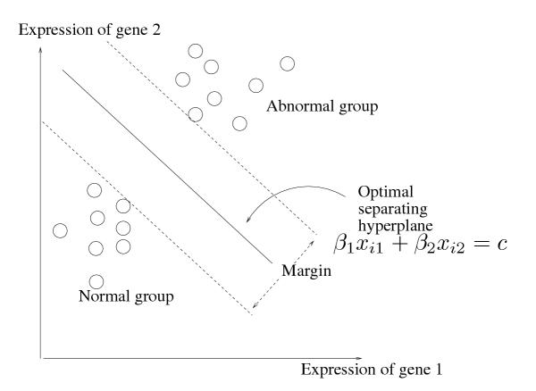
Schematic of the margin classifier.

For a given tumor sample, the output of this classifier is a weighted vector of genes whose combined expression is larger in this sample compared to all normal samples. This would serve as a discriminatory feature set for this tumor sample. Our main goal is to cluster tumor samples of a certain histological type (like CNS or renal) based on the similarity of their feature sets, to identify sub-groups for which the same feature set is discriminatory. This would produce feature sets of moderate size, which find, and effiectively characterize cancer classes with respect to the genes whose detected expression in the tumors distinguishes them from normal cells/tissues. We propose a method that combines margin classification with hierarchical clustering and convex polytope exploration techniques to find cancer classes, and moderately large feature sets of genes for each class, spanning the various gene classes that distinguish the cancer type. We call this procedure Discriminative Margin Clustering.

The input to our procedure is the set of tumor samples, (either labelled with their histological type, like CNS, renal, etc, or unlabeled samples) and the set of normal samples. We run the discriminative margin clustering procedure on the set of tumor samples versus all the normal samples (this is a binary problem, and not a multi-class problem), to obtain sub-types of tumors with similar feature sets. We run the procedure separately on each class of tumor samples (like CNS, renal, etc) to obtain clusters within that class which are similar in terms of their feature sets. The data set and results are present at http://microarray-pubs.stanford.edu/margin clus/. Our method can therefore be run either in a semi-supervised fashion with apriori class labels, or in an unsupervised fashion. We do an empirical validation of the quality of these feature sets in terms of uniqueness to a tumor class by evaluating their goodness on a test set of tumor samples, and show that the accuracy of predicting the correct tumor type is pretty high. The prediction accuracy, though high, is not as good as the accuracy of traditional hierarchical clustering, mainly because we are working with feature sets of small size. Nevertheless, we show (somewhat surprisingly) that small feature sets (which are just based on properties of a certain tumor class versus the normal class) are sufficient to obtain reasonably high prediction accuracies against other tumor classes as well.

Classification

Several researchers have observed that margin classifiers work well in finding signature gene sets for a cancer class. Most previous work [2-6] based on Support Vector Machine classifiers has focused on feature sets (or clusters of feature sets [7]) that either separate a cancer class from all other cancer classes, or that separate a cancer class from the corresponding normal class, by minimizing the Euclidean norm of the feature vector. Several tumors have natural sub-types [8,9] which clustering techniques can identify, but which these classification schemes do not identify (refer [10] for a detailed discussion of this issue, along with additional references to literature). The main difference between our work and previous work on clustering is that our clustering effort is focused on finding sub-types which are amenable to similar diagnostic/therapeutic methods, rather than finding sub-types which are histologically similar. The linear margin classifier we present has been previously studied in [11]. A feature of this classifier is that the discriminatory gene sets are of very small size (this is a property of linear classifiers, where the size of the feature set is provably no more than the number of tumor and normal samples.) Our work differs from previous work in focusing on positive margin classifiers, since the feature sets which result are potentially useful for the purposes of diagnosis and therapy.

Methods like Partial Least Squares [12] can be used to reduce the dimension of the feature space before applying our clustering procedure. It would be interesting to observe how such an approach would affect the quality of clustering and the relevance of the feature sets.

Clustering

A related objective is to group tumor samples with related feature sets. For this purpose, we need to cluster the tumor samples into groups so that tissues within a group have similar feature sets. Traditional methods of clustering tumors [13] use the notion of dot-product or Euclidean distance similarity between the gene expression vectors as the notion of similarity. Clustering based on overall gene expression patterns works very well in grouping together histologically similar tumor samples. However, a problem with this approach is that a disproportionate amount of weight is given to a set of genes which form part of the same broad biological function, like respiration or the cell cycle. The individual genes in these functionally themed groups need not be not discriminatory in the sense we want them to be. It is therefore not geared towards recognizing samples with similar feature sets.

Statistical methods

An alternative method to finding feature sets is to list the genes that are relatively highly expressed in the tumor class as compared to most normal tissue samples, using some standard statistical significance test [14]. The problem with this approach is that for a large set of genes, the normal tissues in which that gene is relatively highly expressed could be the same. Therefore, the set of genes might work well to distinguish a tumor from most normal tissues, but consistently fail to distinguish the tumor class from a particular set of normal tissue samples. For example, for breast cancer samples, most of the genes (more than a thousand) with large expression values would also have large expression in normal breast samples. Thus a set of genes that distinguish breast cancers from most normal tissues will generally do a poor job of discriminating breast cancers from normal breast tissue. The validity of these methods oftentimes depends on the relative abundance of samples of the various normal tissue types; our method does not suffer from this drawback.

Related work

The work of [10] is most similar to our effort. The authors use a completely unsupervised self organizing map technique to cluster gene expression vectors, and identify tumor and normal classes in the SOM. The SOM also provides an expression vector unique to each tumor class. The authors report poor accuracy in classifying breast, ovarian, coloretical and lung cancers, and the feature sets produced for these classes are small in size. Our work differs from their work in being semi-supervised (though it is possible for our method to be run in a completely unsupervised fashion); we start with class labels for each broad tumor class (like CNS, renal, etc) and the set of normal samples. Our method uses an entirely different idea and is geared towards finding specialized subtypes within each histological type which are similar in terms of discrimination. Our clustering procedure finds biologically meaningful sub-types for Breast and Ovarian cancer, where we identify genes like ERBB2, ESR1, NAT1, GATA3 and MSLN as being prominent in the feature sets. These genes are well known markers for these cancer types. We identify three natural sub-types of breast cancer which traditional hierarchical clustering also identifies. In contrast to the traditional hierarchical clustering method, our method relies on very small feature sets to identify the exact same sub-types. In other cases, our method groups tumors differently from the traditional methods. Our classification results have around 75% accuracy for most cancer types except pancreas, prostate and gastric cancer, which is comparable to the 80% accuracy obtained by [10] (a caveat is that we are working with different data-sets, and this may effect the results of the predictions). However, we have the advantage of finding different clusters in some cases (for instance, breast cancer and ovarian cancer), and also finding a different set of markers, some of which have been verified in literature. In addition, we expect our method to produce results even when the class of normal tissues is extremely heterogeneous, with very few samples of any histological type. This suggests our approach as an alternative procedure which may work better in some situations.

The work of Dettling and Buhlmann [15] attempts to cluster genes based on multiclass discrimination of cancer types. We differ in attempting to cluster samples in each tumor type based on similarity of the discriminatory genes. We therefore get multiple clusters of genes for the same broad cancer type, which would reveal fine grained variations within that cancer type.

We emphasize that traditional classification and clustering procedures would be expected to have higher prediction accuracy for unknown samples because they rely more on overall gene expression patterns (this is confirmed in [10]); our clustering method is oriented towards grouping tumors based on similarity of feature sets, so as to identify highly specialized tumor sub-classes. We show that these feature sets have sufficient classifying power to make them statistically meaningful. In some cases, for instance, breast cancer samples, our clustering result mirrors that of traditional hierarchical clustering. In some other cases, for instance, lung cancer, our procedure groups tumor samples of diverse histo-logical origin together, suggesting that a similar marker set or treatment may be amenable to them. In addition, it would also suggest the lack of a common treatment for a set of samples which are histologically similar. There are alternative techniques to achieve the same goal, for instance [10]; the high dimensionality of the gene space often leads to different results from different methods, and a combination of these methods may lead to biologically meaningful insights.

Although this work focusses on the application to global gene expression data and cancer, the discriminative margin clustering method should be generally applicable to large high dimensional data-sets in which similar classification questions arise. For more details on the relevance of our objective, and the manner in which traditional clustering and classification procedures fail to address it, along with additional references to literature, we refer the reader to [10].

Results

Discriminative Margin Clustering

We once again refer to our example from the previous section. The "abnormal" samples in Figure 1 lie near each other, and hence are well separated from the normals by a single line. This will not always be the case: and it hence it is of interest to group members of the abnormal class with respect to their joint separability. This is the idea of discriminative margin clustering.

The process follows the same general scheme as agglomerative hierarchical clustering, but uses margin from the normal class, rather than similarity of expression profiles, as the clustering metric. The idea is schematized in Figure 2.

Figure 2.

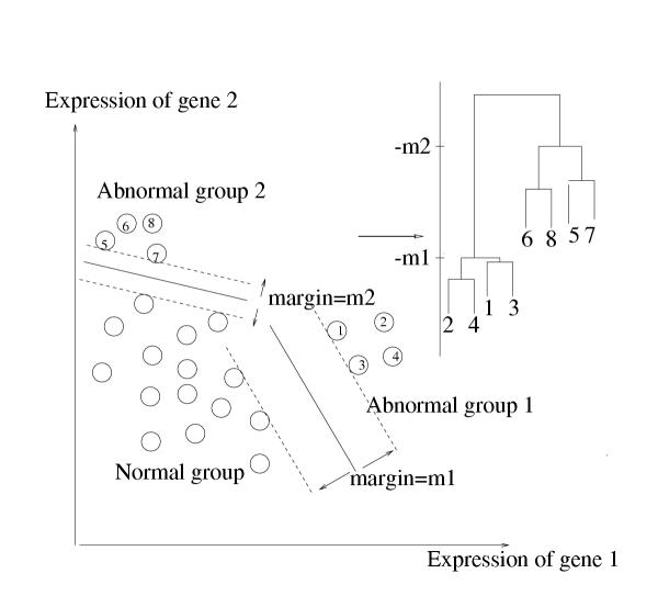
Schematic of discriminative margin clustering.

We start with each abnormal sample forming its own group. Then for every pair of samples, we compute the maximum positive margin classifier for that pair versus the normal samples. We find the pair whose resulting margin is largest, and agglomerate them together. This process is repeated, and at each stage agglomerating the pair of single samples or groups that produces a combined group with largest margin.

Figures 3 and 4 show a toy example. There are 100 genes and 20 samples, 10 each of the normal and abnormal classes. This example is to illustrate the power of our clustering method in finding specialized tumor sub-types which other clustering methods would miss out. This example is not a stochastic model of gene expression, and is presented mainly to illustrate the potential difference in hierarchical clustering and discriminative margin clustering in terms of the sub-types they are capable of detecting. Discriminative margin clustering will detect highly specialized sub-types with similar feature sets, while hierarchical clustering will detect tumor types with similar gene expression patterns. Both methods therefore have their relative merits.

Figure 3.

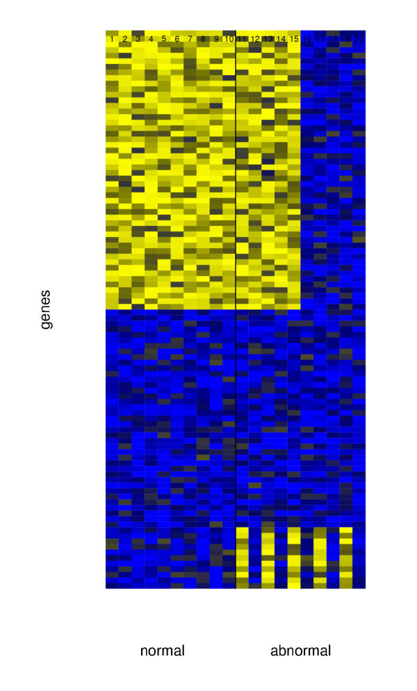
Heatmap for the toy example.

Figure 4.

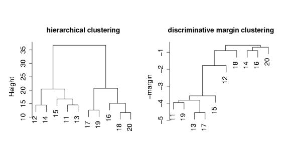
Dendograms for hierarchical and discriminative margin clustering on the toy example.

The first 50 genes have high expression for the normal samples and abnormal samples 11–15, and lower expression for samples 16–20, while the last 10 genes have high expression for samples 11,13,15,17 and 19 and low expression for the others. The left panel of Figure 4 shows average linkage hierarchical clustering, using the Euclidean metric. The first 50 genes dominate the clustering, and hence samples 11–15 and 16–20 represent the major groups found. The right panel of the figure shows the result of discriminative margin clustering. It has separated samples 11,13,15,17,19, as these are the ones most easily discriminated from the normal class. Each join of the dendrogram is drawn at height equal to the (negative) margin achieved for the combined groups.

This discriminative margin clustering procedure delivers another useful piece of information. At each merge, it finds a set of non-negative gene weights that best separate the current group from the set of normals. In practical terms, this might mean that each successive cluster defines a group of cancers for which a specific combination therapy (directed at the products of the genes that best distinguish this group of tumors from all normal tissues) would be useful.

For example the join at height = -3.6 has weight vector

(0.14, 0.00, 0.27, 0.07, 0.00, 0.00, 0.14, 0.17, 0.00, 0.21, 0.00)

for the last 10 genes, and zero for the rest. Hence in this example we would learn that the separation of samples 11, 13, 15, 17, and 19 is best achieved by a (weighted subset of) genes 90–100.

The dendrogram from this process can also be used for classification of new samples. Given a new expression profile z = (z₁, z₂, ... z_p), at each join in the tree we compute the margin where the are the estimated gene weights. The margin for z is defined to be the largest value m such that z achieves a margin of m at a join at or below height -m of the tree. If the margin m is negative, it is set to -∞.

The predicted class is "abnormal" if m is greater than some cut-point h, and "normal" otherwise. Hence samples with margin -∞ are always predicted as "normal". The optimal cut-point h is estimated from a test set or cross-validation.

Figure 5 shows the training and test error curves for the toy example. A test sample of size 500 was used. An "error" would be the classification of a normal sample as "abnormal", or vice-versa. The test error is minimized at a margin about 2.0, which is reasonable in view of the dendrogram of Figure 4. Therefore, we can obtain clusters of the "abnormal" samples by chopping the tree at a margin of 2.0.

Figure 5.

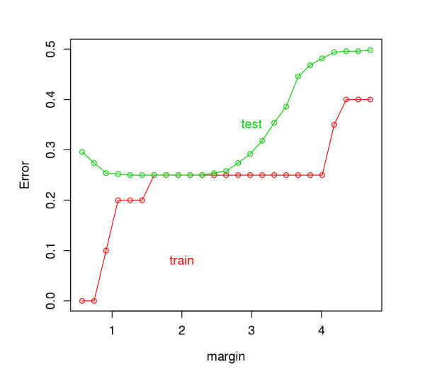
Training and test errors for the toy example.

The clustering procedure therefore has the potential of finding highly specialized tumor sub-types. These groups would be expected to have useful information in terms of diagnosis and therapy.

Discussion

Although it would appear that our clustering procedure simply groups together samples based on the similarity of the maximum margin feature sets, this is not strictly true. The similarity between two tumor samples could be very high even if the maximum margin feature sets have low overlap. All we require is that there exist a common feature set which gives large margin for both the samples. Therefore, our clustering procedure is different from the more simple-minded procedure that computes similarity between the maximum margin feature sets. Therefore, if a set of tumor samples has a common discriminatory feature set (this need not be the maximum margin feature set for any of the samples individually), our clustering procedure would be expected to group them together. This explains why it performs well in classifying unknown samples in the cross-validation test we describe in the next section.

One advantage of clustering is removal of sensitivity to noise. Though expression values of a particular tumor sample may be prone to error, the combined margin classifier for a class of related tumor samples would be a reliable indicator of the genes which characterize the class. For a gene to be erroneously included with large weight in the feature set, its expression value has to be abnormally high in most of the samples in the class. This is a possibility if the class has only one sample, but this event has low probability if the class has many samples. This point also illustrates the importance of finding a weighted combination as opposed to an unweighted combination. Genes with large weight are more reliable markers than genes with small weight. For instance, ERBB2 appears as a gene with a large weight for a large cluster of breast samples, and therefore, would be a good candidate to include in the feature set. We also note that (contrary to intuition) finding the best weighted combination is a computationally simpler problem than finding the best un-weighted combination (which is provably computationally intractable). We therefore focus our attention on computing weighted combinations; we discuss how our results change for unweighted combinations in the next section.

One natural question to ask is what if the margin is negative. Our experiments with the tumor and normal data set which we present in the next section shows that even if we consider the entire class of tumors versus the entire class of normals, the maximum margin is positive, showing that there exists a set of discriminatory genes for this case as well. A similar result is obtained by [10]. We will therefore assume that the margin is always positive.

We note that though the set of genes yielding the largest possible margin is unique, there will be many sets of genes whose weighted combinations yields close to the largest margin. In Appendix B, we discuss techniques to find larger feature sets which yield close to the maximum margin. This has potential applications to finding diagnostic/therapeutic markers. We note that in our experiments with the tumor and normal dataset, the maximum margin feature set is contained in the expanded feature set, albeit with smaller weights assigned to the corresponding genes.

Properties of the feature sets and expanding them

For a realistic look at its potential application to real biological problems, we apply discriminative margin clustering to a large dataset of gene expression data from systematic analysis of transcript levels in normal and cancer tissues, using DNA microarrays. We use data from the Stanford Microarray Database [16]. The log scale, mean centered and normalized dataset can be found at http://microarray-pubs.stanford.edu/margin clus/. We impute missing values using the k-nearest neighbors method with k = 10. For our method, accurate imputation of missing values is important. We set all remaining missing values to zero.

Since we wish only to cluster samples which have the same broad histological type (for instance, lung samples or ovarian samples), we run the clustering procedure separately on each broad tumor class versus all the normal samples. There are 104 normal samples and 268 tumor samples which fall in 14 broad tumor classes – Bladder, Breast, CNS, Kidney, Liver, Lung, Lymph, Ovary, Pancreas, Prostate, Skin, Soft tissue, Stomach and Testis. There are around 7500 genes, and the data is on the log scale.

Figure 6 illustrates the discriminative margin clustering for a collection of lung samples. Note that the clustering groups the squamous, adeno and small cell sub-types separately, but the large cell sub-type does not cluster as a discrete group suggesting that these tumors are heterogenous with respect to the molecular features that distinguish them from normal tissues. Combining the large cell subtype together results in a feature set with very small margin, showing the absence of a common set of molecular markers. We note that traditional hierarchical clustering using a dot-product similarity measure would group the large-cell sub-type together, which shows these samples have similar overall gene expression patterns and histological type. But, for the purpose of finding discriminating feature sets, these samples are very heterogeneous.

Figure 6.

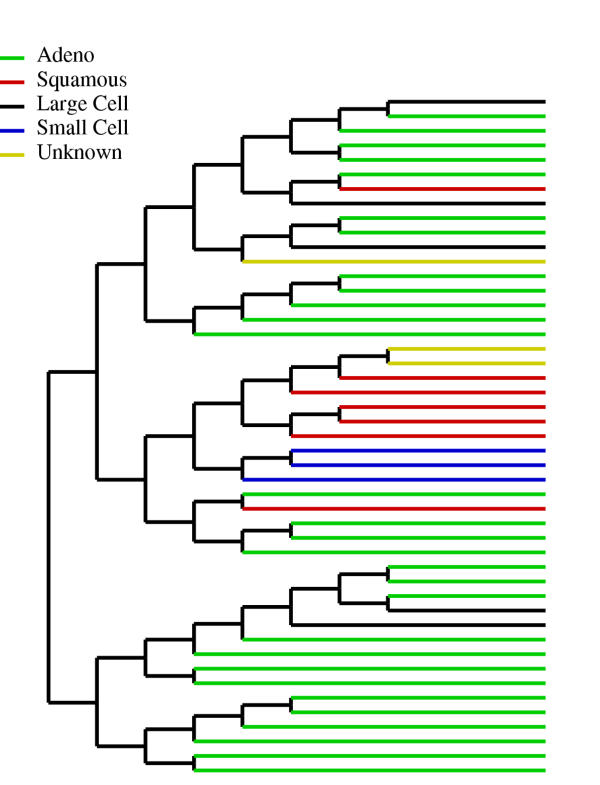
Dendogram for the lung samples. Note that there is no common feature set for the large cell sub-type, though traditional hierarchical clustering groups these samples together. Also, the sub-groups for the other classes are different from those produced by traditional clustering methods.

Cancers of the same histological type can be heterogenous in their gene expression patterns, their genetic origin and their behavior. Therefore, we do not expect the discriminating gene set to be consistent among cancers of the same histological diagnosis. Nevertheless, we tested the ability of discriminative margin clustering to define gene expression features useful for classifying cancers according to broad histological types. We do a predictive analysis for the quality of the clustering produced using the identification of known cancer classes as a test. We describe the procedure below.

To obtain clusters from the dendogram, we need to find the margin at which to chop the tree. We do a cross-validation test by randomly partitioning the samples into two-third "training" and one-third "test" groups. We run the discriminative margin clustering procedure on each tumor class in the training set versus the normal samples in the training set. This yields one dendogram for each tumor class. For each sample in the test set, we find the node with the best margin among all dendograms generated from the training data. This would assign a predicted class for the test sample as CNS, renal, normal, etc, along with the margin. Figure 7 shows the predicted class of each tumor and normal sample; the color assigned to a point is the color of the predicted class. A margin of -∞ implies classification as normal. From this figure, it we can deduce that a margin of 2.0 is the threshold beyond which the classification accuracy is large. To confirm this, we fix a margin, and chop the trees off at that margin to obtain a larger set of trees. Now, we re-classify the test samples using the nodes in the new trees (all nodes have margin at least the cut-off now). Figure 8 shows the error in accurately classifying the normal and tumor samples in the test set. The error is minimized when the margin is 2.0. We therefore pick this as the margin.

Figure 7.

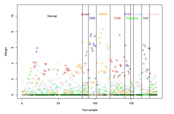
Margin for the test samples along with the label of the cluster which yields the largest margin. The vertical lines separate the actual classes of the test samples, while the color of the points illustrate the predicted class.

Figure 8.

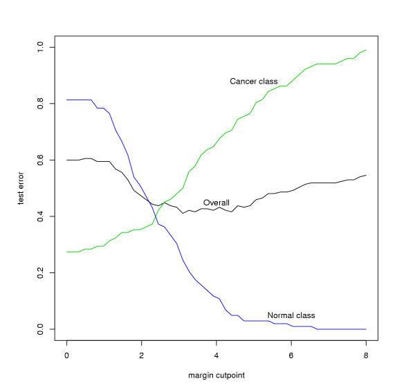
Training and test errors for the samples.

For the margin of 2.0, Table 1 shows the prediction of the test samples. Note that the accuracy of prediction is around 75% for most classes, but bad for prostate, pancreas and stomach cancer. The normal samples cannot be predicted accurately as they are extremely heterogeneous in nature (there are very few samples for most histological types), and if the training set misses out the normal sample of a particular histological type, the feature sets may not classify the test samples corresponding to that type correctly. Despite this heterogeneity, the accuracy for predicting the tumor samples is comparable to that in [10] (they use a data set with comparable number of normal and tumor samples), and as we show below, the feature sets have genes which are biologically relevant for that cancer class. We then consider the prediction of the test sample using just the dendograms of the corresponding histological type. This would predict whether the test sample belongs to that histological type or whether it is a normal sample. This improves the prediction results (Table 2). Note that the power of the clustering in predicting broad histological type is high, even though this analysis did not take into account the considerable molecular heterogeneity within the cancer classes.

Table 1.

Test set prediction results for all classes

	Predicted class
True class	Normal	Breast	CNS	Kidney	Lung	Ovary	Panc.	Prostate	Soft	Stom.	% correct
Normal	28	1	2	15	15	0	2	8	1	11	34
Breast	0	5	0	0	0	0	0	1	0	2	62
CNS	2	0	7	2	0	0	0	0	0	0	64
Kidney	1	0	0	17	0	0	0	0	0	1	89
Lung	4	1	0	0	14	0	0	1	0	0	70
Ovary	1	0	0	0	1	6	0	0	0	0	75
Pancreas	4	0	0	0	0	0	0	0	0	0	0
Prostate	9	0	0	0	0	0	0	0	0	0	0
Soft Tissue	0	0	1	0	1	0	0	0	9	0	82
Stomach	5	0	0	0	1	0	0	0	0	4	40

Table 2.

Test set prediction results for each class versus normal only

	Predicted class
True class	Normal	Breast	CNS	Kidney	Lung	Ovary	Panc.	Prostate	Soft	Stom.	% correct
Normal	NA	3	2	24	16	0	15	71	1	58	75
Breast	3	5	0	0	0	0	0	0	0	0	62
CNS	2	0	9	0	0	0	0	0	0	0	82
Kidney	0	0	0	19	0	0	0	0	0	0	100
Lung	4	0	0	0	16	0	0	0	0	0	80
Ovary	2	0	0	0	0	6	0	0	0	0	75
Pancreas	1	0	0	0	0	0	3	0	0	0	75
Prostate	0	0	0	0	0	0	0	11	0	0	100
Soft Tissue	1	0	0	0	0	0	0	0	10	0	91
Stomach	0	0	0	0	0	0	0	0	0	10	100

We obtain similar classification accuracy even if we make the weights of the genes in the feature set equal to 1. This shows that the combination of genes is important in addition to the weights, and for a given set of expression values, the discriminatory feature sets are not very sensitive to the weights. However, the weighted combination is more resilient to noise in the data than the unweighted combination, especially since we are considering sets of small size.

We note that traditional classifiers, for instance, the nearest neighbor classifier (which we have implemented and compared against), have higher prediction accuracy (refer [10]), as they are based on broader gene expression profiles. Our method, in contrast, is geared towards finding tumor sub-types which are similar in terms of having the same small discriminative set of genes, and we use just these for classification to test the significance of these genes. These discriminative sets also make no explicit effort to discriminate one cancer class from another – we simply discriminate the cancer class from the normal samples. Our main point is to find clusters of specialized tumors with a common marker set. We show, somewhat surprisingly, that these feature sets have the additional power to classify unknown tumor samples well, implying that they have statistical validity.

In some cases, the clustering helps us identify natural tumor sub-types as well. For instance, breast cancer samples cluster into three natural sub-types, which are also identified by traditional hierarchical clustering.

ERBB2 sub-type

The feature set for this class gives 65% weight to ERBB2.

Luminal A sub-type

ESR1, NAT1 and GATA3 together account for 55% of the weight in the feature set.

Proliferative sub-type

Characterized by large expression values for cell-cycle related genes, suggesting a rapidly proliferating sub-type.

The feature sets of genes produced at the nodes of the cluster tree are small (about 10 genes) even at the top nodes of the tree. Though these feature sets include genes which are well studied in the context of their respective cancers, these sets may be too small to provide a sufficient set of candidates for diagnosis or treatment. For example, for a breast cancer class with 15 samples, the feature set (along with the associated weights) is listed in Table 3. Although the maximum margin feature set is small, there will be feature sets with close to the optimal margin, which are equally good candidates for finding markers. Note that the presence of these feature sets does not affect the clustering, but simply yields more marker sets.

Table 3.

Feature set for a breast cancer cluster.

	Weight	Gene Name
1	0.006	LGALS4
2	0.222	ERBB2
3	0.034	ESR1
4	0.080	GATA3
5	0.118	OSF-2
6	0.014	EVI2A
7	0.049	VAV3
8	0.057	HS1-2
9	0.096	NUF2R
10	0.066	C20ORF1
11	0.019	TOPK
12	0.075	HNF3A

We can expand the set of genes by convex programming techniques. At a particular node in the cluster tree, we consider the polytope of all feature sets whose margin is close to the optimal margin (the "closeness" being a parameter which we can control). We then formulate a quadratic program to search for a combination in this polytope that includes as many different genes as possible. Details can be found in Appendix B. These feature sets provide a much larger set of potential markers. In our experiments, the maximum margin feature set is contained in the expanded feature set, albeit with smaller weight.

For the breast cancer cluster in represented in Table 3, the expression patterns for the expanded list of genes are shown in Figure 9, (and in more detail in the web supplement) in heatmap format. Adjacent to each gene is the weight assigned to it in the expanded feature set. For each tissue, we also indicate the weighted expression value of the genes in the feature set. The first 15 samples are breast cancer samples while the rest are normal tissue samples. Please refer to the web supplement for an enlarged version of this figure. We have clubbed two sub-classes found by the clustering in this heatmap. Note that the ERBB2 sub-type (last 4 tumor samples) has high expression of ERBB2, GRB7, MLN64 and LIV-1, while the Luminal A sub-type (remaining samples) has high expression of ESR1, NAT1 and LIV-1. The expression patterns of these genes is sufficient to discriminate these two sub-types from each other.

Figure 9.

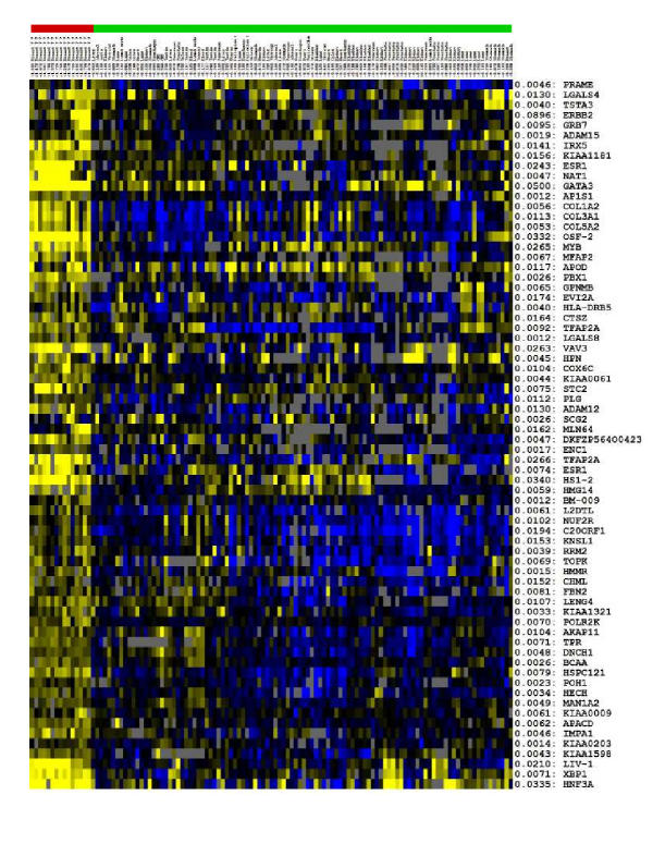
Heatmap for the expanded gene-list of a breast cancer sub-type. Note the spread of expression values in the normal samples. Also note that ERBB2, GRB7 and LIV-1 define one sub-class, while ESR1 and NAT1 define the other sub-class.

Many genes related to proliferation and the cell cycle (C20ORF1, TOPK, L2DTL, KNSL1, NUF2R, CENPF, ...) are present in the expanded feature set. These genes do not have very high differential expression values, and are relatively highly expressed in many cancer types. They are therefore not present in the maximum margin feature sets that drive the clustering procedure, though they are present in the expanded feature sets. On another note, GRB7, which is significantly co-expressed with ERBB2, is absent in the maximum margin feature set, but is present in the expanded feature set.

The heatmap clearly illustrates the spread of expression values in the normal tissue sample. For any one normal sample, the number of highly expressed genes is relatively small, but for any gene, the probability that at least one normal tissue expresses the gene at a level comparable to that in the given tumor is high. Nevertheless, this example shows that we can find a set of genes that as a group, discriminates the tumor class from the normal classes quite well.

Although our analysis used no information about the known diagnostic or therapeutic value of the genes, the feature sets identified were strikingly enriched in genes corresponding to the established therapeutic and diagnostic targets. We illustrate these in Table 4. For example, ERBB2 and ESR1 are targeted by some of the most effective treatments for breast cancer. The genes MSLN and AMACR have been identified as useful markers of Ovarian and Prostate cancers respectively, and our feature sets are heavily weighted in favor of these genes. Note that despite some similarity, many of our markers are quite different from those in [10]. This may be because of the fact that we use different data-sets.

Table 4.

Verified markers for some tumor types in the feature sets.

Tumor Class	Marker Genes
Breast	ERBB2, GRB7, NAT1, ESR1, GATA3
CNS	FABP7, VEGF
Renal	IGFBP3, VEGF
Pancreas	DAF, LGALS4, CTSD, MMP14
Ovarian	MSLN, PAX8
Prostate	AMACR

A detailed collection of dendograms and feature sets are present at http://microarray-pubs.stanford.edu/margin clus/.

Discussion

We have illustrated a procedure for identifying interesting feature sets of genes to distinguish a tumor class from a set of normal tissues from large scale systematic gene expression data sets, obtained by DNA microarrays. This method has wider applicability in finding feature sets to discriminate one set of data samples from another. The method has the advantage of producing feature sets of moderate size (neither too small nor too large), while at the same time discriminating the tumor class from all normal classes. The method involves a novel hierarchical clustering procedure combined with polytope exploration techniques. The clustering diminishes sensitivity of the results to noise, while the margin classifier technique gives equal weightage to discriminating the tumor class from all normal samples. The method may be especially valuable in identifying clinically useful sets of diagnostic or therapeutic markers for defined groups of cancers.

An interesting research direction which we plan to pursue is to use the results of the margin classifier to find combinations of genes whose protein products can be targeted by antibodies. This strategy may be useful in developing screening tests and drug treatments for cancers.

Paper web-site

http://microarray-pubs.stanford.edu/margin clus/

Methods

A Details of the Margin Classifier

For clarity of exposition, let us denote the set of tumor tissues by T, and a set of normal tissues by N. For every tissue t ∈ T and n ∈ N, we are given the expression values of the set G of genes. For every gene, g ∈ G and tissue, x ∈ T ∪ N, let e_xg denote the expression of gene g in tissue t. These expression levels are on the log scale.

Our goal is to find feature sets for the tumor tissue samples using the following general framework. Suppose for a subset T' ⊆ T, there exists a set of fractional weights w = {w_g|g ∈ G, Σ_g∈Gw_g = 1} such that the minimum weighted expression of the genes in every t ∈ T', given by E_wT' = min_t∈T' Σ_gw_g·e_tg is much larger than the maximum expression of the weighted expression of the genes in any normal tissue, given by E_wN = max_n∈N Σ_gw_g·e_ng. In other words, the difference (note that we are working in the log scale) r_wT' = E_wT' -E_wN is large. This means, for example, that a drug combination whose activity is directed at the products of the genes by the weighted combination w could target the tumor tissues more effectively than any normal tissue, and therefore would, in principle, be effective in chemotherapy.

The goal is to make the difference of r_T'w as large as possible by choosing an appropriate w. We call r_T' = max_wr_wT', the effectiveness value for tissues T'. The w which maximizes r_T'w is the feature set of the tumors T'. Given t ∈ T', the goal of finding w can be reduced to a linear program as follows:

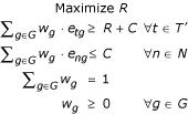
The feature set is the set G' = {g|w_g > 0}. This linear program is precisely the one used for finding separating hyperplanes minimizing the l₁ norm in linear Support Vector Machines [1]. This contrasts to the non-linear approach is used in [5] for cancer classification. A similar linear programming approach is used by [11] to find small feature sets in gene expression data. We show later how to construct feature sets of variable sizes and confidence using our methods.

It is possible to construct examples where the best margin is negative, i.e., the classes overlap, but this never happened in all of our examples with real gene expression data. A feature of a linear classifier is that the number of nonzero weighted genes is at most the number of samples in the data-set. In our experiments, the number of genes with non-zero weight is typically much smaller than this upper bound.

We use a simplex method (available in the CPLEX commercial package) to solve this problem for each candidate merge. The idea behind the simplex algorithm is to iteratively modify the weights using an approach similar to gradient descent, as long as the objective function improves. It can be shown that the algorithm converges in a small number of steps, especially for problems of the form we discuss, which are called packing linear problems. The intuition behind the small number of steps is that the algorithm can easily find a direction in the gene space in which a large alteration in weights improves the objective function significantly while maintaining feasibility of the problem.

Let M(t) be the achieved margin for sample t, M({t₁, t₂}) is the margin for the pair of samples t₁, t₂ etc. A key fact here is that merging samples cannot increase the margin

M({t₁, t₂}) ≤ min [M (t₁), M (t₂)]    (1)

This allows us to draw the tree with join heights equal to the negative margins.

A computationally simpler approximation we use, which produces the same clustering results is the following:

M({T₁, T₂}) ≈ min [M (T₁), M (T₂), min{M (t₁, t₂), t₁∈ T₁, t₂∈ T₂}]    (2)

This says that the margin achieved in joining groups T₁, T₂ is the minimum margin for each of the two groups, and all pairs of samples, one in group T₁ and the other in group T₂. The left hand side of (2) must be less than or equal the right hand side, and in general this seems to be a reasonable approximation. It allows us to find the best probable pair using only quantities that have already been computed. Note that as long as the clustering results are the same, the feature sets we find using the simpler approximation would be the same as those found using the original scheme, and this is what we observe in practice.

Finding competitors at each join in the tree

The linear program mentioned above has the problem of reporting a relatively small set of genes. It would miss out genes which are heavily weighted in some distinct feature set whose margin is close to the optimal one.

It is therefore desirable to have routines that "search" around the optimal solution to find other good feature sets. We present several approaches which find feature sets of varying sizes, with a concrete confidence measure on the importance of each set. It is also easy to incorporate additional constraints, like insisting certain genes are present to a minimum fraction, in our methods.

The first step in this process is to relax the margin slightly and define a new polytope where any weight vector is a "good" weight vector.

Suppose ε is the relaxation in the margin. Choosing a larger value of ε would yield a larger set of possible feature sets to choose from, but the margin obtained from these would be lower, implying lesser confidence in the set. For our data-set, ε = 0.4 produces feature sets of moderate size (50 – 100 genes).

For a set of samples T', let M(T') = R. The polytope P_ε (T') is defined as:

Our goal now is to find weight vectors in P_ε (T') with large number of non-zero dimensions (genes). We outline two methods below.

Non-Linear programming approach

Our first approach is to solve the following program:

Though the objective function is non-linear, it is convex, and therefore can be optimized using interior point methods. The CPLEX barrier optimizer can optimize for this function.

The advantage of this function is that it "spreads" the weight over many genes and typically gives a much larger feature set than the maximum margin feature set.

Minimum overlap method

In this method, we start with a set of genes G' and iteratively expand this set by finding extreme points with minimum overlap with this set. Given any starting extreme point with gene set G', consider the following linear program:

This will find a weight vector whose total weight along the dimensions G' is as small as possible. Let G" = {g ∈ G|w_g > 0}. We set G' ← G' ∪ G", and iterate.

We can stop when the objective value stops changing substantially. This technique quickly finds a large set of important genes.

This method has an added advantage. Given any feature set, if we set G' to be this set, the objective value of the linear program tells us the minimum fraction to which genes in this set must be present in any weight vector in the polytope P_ε(T'). This can be used as a confidence measure of the feature set.

We tested the algorithms on a group of 3 Breast tumors, with ε set to 0.4. We find the confidence of a feature set using the program described above. The maximum margin feature set with 8 genes has confidence (as defined above) 37%. The non-linear technique produces a larger feature set of around 30 genes with confidence of 70%, which is a much larger confidence than the solution produced by the maximum margin classifier.

References

- Vapnik V. The Nature of Statistical Learning Theory. Springer-Verlag; 1995. [Google Scholar]
- Brown M, Grundy W, Lin D, Cristianini N, Sugnet C, Furey T, Ares M, Jr, Haussler D. Proc Natl Acad Sci. 2000;97:262–267. doi: 10.1073/pnas.97.1.262. [DOI] [PMC free article] [PubMed] [Google Scholar]
- Golub TR, Slonim DK, Tamayo P, Huard C, Gaasenbeek M, Mesirov JP, Coller H, Loh ML, Downing JR, Caligiuri MA, Bloomfield CD, Lander ES. Science. 1999;286:531–537. doi: 10.1126/science.286.5439.531. [DOI] [PubMed] [Google Scholar]
- Moler E, Chow M, Mian I. Physiol Genomics. 2000;4:109–126. doi: 10.1152/physiolgenomics.2000.4.2.109. [DOI] [PubMed] [Google Scholar]
- Ramaswamy S, Tamayo P, Rifkin R, Mukherjee S, Yeang C-H, Angelo M, Ladd C, Reich M, Latulippe E, Mesirov JP, Poggio T, Gerald W, Loda M, Lander E, Golub TR. Proc Natl Acad Sci. 2001;98:15149–54. doi: 10.1073/pnas.211566398. [DOI] [PMC free article] [PubMed] [Google Scholar]
- Su A, Welsh J, Sapinoso L, Kern S, Dimitrov P, Lapp H, Schultz P, Powell S, Moskaluk C, Frierson H, Jr, Hampton G. Cancer Res. 2001;61:7388–93. [PubMed] [Google Scholar]
- Jornsten R, Yu M. Bioinformatics. 2003:1100–1109. doi: 10.1093/bioinformatics/btg039. [DOI] [PubMed] [Google Scholar]
- Garber ME, Troyanskaya OG, Schluens K, Petersen S, Thaesler Z, Pacyna-Gengelbach M, van de Rijn M, Rosen GD, Perou CM, Whyte RI, Altman RB, Brown PO, Botstein D, Petersen I. Proc Natl Acad Sci. 2001;98:13784–9. doi: 10.1073/pnas.241500798. [DOI] [PMC free article] [PubMed] [Google Scholar]
- Perou CM, Sorlie T, Eisen MB, van de Rijn M, Jeffrey SS, Rees CA, Pollack JR, Ross DT, Johnsen H, Akslen LA, Fluge O, Pergamenschikov A, Willimas C, Zhu SX, Lonning PE, Borresen-Dale A-L, Brown PO, Botstein D. Nature. 2000;406:747–752. doi: 10.1038/35021093. [DOI] [PubMed] [Google Scholar]
- Covell DG, Wallqvist A, Rabow AA, Thanki N. Molecular Cancer Therapeutics. 2003;2:317–332. [PubMed] [Google Scholar]
- Grate LR, Bhattacharyya C, Jordan MI, Mian IS. Workshop on Algorithms in Bioinformatics. 2002.
- Nguyen DV, Rocke DM. Bioinformatics. 2002:39–50. doi: 10.1093/bioinformatics/18.1.39. [DOI] [PubMed] [Google Scholar]
- Eisen M, Spellman P, Brown PO, Botstein D. Proc Natl Acad Sci. 1998;95:14863–68. doi: 10.1073/pnas.95.25.14863. [DOI] [PMC free article] [PubMed] [Google Scholar]
- Tusher VG, Tibshirani R, Chu G. PNAS. 2001;98:5116–21. doi: 10.1073/pnas.091062498. [DOI] [PMC free article] [PubMed] [Google Scholar]
- Dettling M, Buhlmann P. Genome Biology. 2002;3:research0069.1–0069.15. doi: 10.1186/gb-2002-3-12-research0069. [DOI] [PMC free article] [PubMed] [Google Scholar]
- Sherlock G, Hernandez-Boussard T, Kasarskis A, Binkley G, Matese JC, Dwight SS, Kaloper M, Weng H, Jin S, Ball CA, Eisen M, Spellman PT, Brown PO, Botstein D, Cherry JM. Nucleic Acids Res. 2001;29:152–5. doi: 10.1093/nar/29.1.152. [DOI] [PMC free article] [PubMed] [Google Scholar]