Quantifying causal emergence shows that macro can beat micro

Significance

Properly characterizing emergence requires a causal approach. Here, we construct causal models of simple systems at micro and macro spatiotemporal scales and measure their causal effectiveness using a general measure of causation [effective information (EI)]. EI is dependent on the size of the system’s state space and reflects key properties of causation (selectivity, determinism, and degeneracy). Although in the example systems the macro mechanisms are completely specified by their underlying micro mechanisms, EI can nevertheless peak at a macro spatiotemporal scale. This approach leads to a straightforward way of quantifying causal emergence as the supersedence of a macro causal model over a micro one.

Abstract

Causal interactions within complex systems can be analyzed at multiple spatial and temporal scales. For example, the brain can be analyzed at the level of neurons, neuronal groups, and areas, over tens, hundreds, or thousands of milliseconds. It is widely assumed that, once a micro level is fixed, macro levels are fixed too, a relation called supervenience. It is also assumed that, although macro descriptions may be convenient, only the micro level is causally complete, because it includes every detail, thus leaving no room for causation at the macro level. However, this assumption can only be evaluated under a proper measure of causation. Here, we use a measure [effective information (EI)] that depends on both the effectiveness of a system’s mechanisms and the size of its state space: EI is higher the more the mechanisms constrain the system’s possible past and future states. By measuring EI at micro and macro levels in simple systems whose micro mechanisms are fixed, we show that for certain causal architectures EI can peak at a macro level in space and/or time. This happens when coarse-grained macro mechanisms are more effective (more deterministic and/or less degenerate) than the underlying micro mechanisms, to an extent that overcomes the smaller state space. Thus, although the macro level supervenes upon the micro, it can supersede it causally, leading to genuine causal emergence—the gain in EI when moving from a micro to a macro level of analysis.

In science, it is usually assumed that, the better one can characterize the detailed causal mechanisms of a complex system, the more one can understand how the system works. At times, it may be convenient to resort to a “macro”-level description, either because not all of the “micro”-level data are available, or because a rough model may suffice for one’s purposes. However, a complete understanding of how a system functions, and the ability to predict its behavior precisely, would seem to require the full knowledge of causal interactions at the micro level. For example, the brain can be characterized at a macro scale of brain regions and pathways, a meso scale of local populations of neurons such as minicolumns and their connectivity, and a micro scale of neurons and their synapses (1). With the goal of a complete mechanistic understanding of the brain, ambitious programs have been launched with the aim of modeling its micro scale (2).

The reductionist approach common in science has been successful not only in practice, but has also been supported by strong theoretical arguments. The chief argument starts from the intuitive notion that, when the properties of micro-level physical mechanisms of a system are fixed, so are the properties of all its macro levels—a relation called “supervenience” (3). In turn, this relation is usually taken to imply that the micro mechanisms do all of the causal work, i.e., the micro level is causally complete. This leaves no room for any causal contribution at the macro level; otherwise, there would be “multiple causation” (4). This “causal exclusion” argument is often applied to argue against the possibility for mental causation above and beyond physical causation (5), but it can be extended to all cases of supervenience, including the hierarchy of the sciences (6).

Some have nevertheless argued for the possibility that genuine emergence can occur. Purported examples go all of the way from the behavior of flocks of organisms (7) to that of ant colonies (8), brains (9), and human societies (10). Unfortunately, it remains unclear what would qualify some systems as truly emergent and others as reducible to their micro elements. Also, most arguments in favor of emergence have been qualitative (11). A convincing case for emergence must demonstrate that higher levels can be causal above and beyond lower levels [“causal emergence” (CE)]. So far, the few attempts to characterize emergence quantitatively (12) have not been based on causal models.

Here, we make use of simple simulated systems, including neural-like ones, to show quantitatively that the macro level can causally supersede the micro level, i.e., causal emergence can occur. We do so by perturbing each system through its entire repertoire of possible causal states (“counterfactuals,” in the general sense of alternative possibilities) and evaluating the resulting effects using “effective information” (EI) (13). EI is a general measure for causal interactions because it uses perturbations to capture the effectiveness/selectivity of the mechanisms of a system in relation to the size of its state space. As will be pointed out, EI is maximal for systems that are deterministic and not degenerate, and decreases with noise (causal divergence) and/or degeneracy (causal convergence).

For each system, we completely characterize the causal mechanisms at the micro level, fixing what can happen at any macro level (supervenience). Macro levels are defined by coarse graining the micro elements in space and/or time, and this mapping defines the repertoire of possible causes and effects at each level. By comparing EI at different levels, we show that, depending on how a system is organized, causal interactions can peak at a macro rather than at a micro spatiotemporal scale. Thus, the macro may be causally superior to the micro even though it supervenes upon it. Evaluating the changes in EI that arise from coarse or fine graining a system provides a straightforward way of quantifying both emergence and reduction.

Theory

In what follows, we consider discrete systems S of connected binary micro elements that implement logical functions (mechanisms) over their inputs. We first introduce a state-dependent measure of causation, the “cause” and “effect information” of a single system state s₀, before we describe the state-independent EI of the system S.

State-Dependent Causal Analysis.

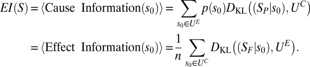
The micro mechanisms of S specify its state-to-state transition probability matrix (TPM) at a micro time step t. Building upon the perturbational framework of causal analysis developed by Judea Pearl (14; see also ref. 18), the TPM can be obtained by perturbing S at t₀ (13) into all possible n initial states with equal probability 1/n [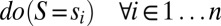 ]. Perturbing the system in this way corresponds to the unconstrained repertoire (probability distribution) of possible causes U^C, and determines the probability of the resulting states at t₊₁, corresponding to the unconstrained repertoire of possible effects U^E. Although U^C is thus identical to the uniform distribution U [with 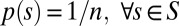], U^E is typically not uniform. A current system state S = s₀ is associated with the probability distribution of past states that could have caused it (“cause repertoire S_P|s₀,” obtained by Bayes’ rule), and the probability distribution of future states that could be its effects (“effect repertoire S_F|s₀”). A system’s mechanisms and current state thus constrain both the repertoire of possible causes U^C and that of possible effects U^E. An informational measure of the causal interactions in the system (15) can then be defined as the difference [here Kullback–Leibler divergence (D_KL) (16)] between the constrained and unconstrained distributions:

Cause/effect information depends on two properties: (i) the size of the system’s state space (repertoire of alternatives), because both are bounded by log₂(n); (ii) the effectiveness of the system’s mechanisms in specifying past and future states. To isolate effectiveness from size, we define the following normalized coefficients: .

The “cause coefficient” describes to what extent a state is sufficient to specify its past causes, and the “effect coefficient” indicates how necessary a state is to specify its future effects (Fig. 1B). In turn, the effect coefficient itself is a function of two terms, “determinism” and “degeneracy” (see Effect Coefficient and Effectiveness (Eff) Expressed as Determinism and Degeneracy for derivation):

The determinism coef. is the difference between the effect repertoire and the uniform distribution (U) of system states, divided by log₂(n), and measures how deterministically (reliably) s₀ leads to the future state of the system: it is “1” (complete determinism) when the current state leads to a single future state with probability p = 1, and is “0” (complete indeterminism or noise) if it could be followed by every future state with p = 1/n. The degeneracy coef. measures to what degree there is deterministic convergence (not due to noise) from other states onto the future states specified by s₀. In broad terms, degeneracy refers to multiple ways of deterministically achieving the same effect or function (17, 18). The degeneracy coef. is 1 (complete degeneracy) when s₀ specifies the same future state as all other states, and 0 when s₀ specifies a unique future state (no degeneracy).

Fig. 1.

Cause and effect coefficients in example systems with different causal architectures. (A) The systems consist of two interconnected binary COPY gates with possible states 0 and 1. (B) A causally perfect system, in which each state has one cause and one effect. Thus, s₀ = [11] has a cause and effect coefficient (coef.) of 1. Moreover, there is no divergence (determinism coef. = 1) and no convergence (degeneracy coef. = 0). (C and D) In both the completely indeterministic and completely degenerate systems, state s₀ = [11] is completely insufficient to specify past system states and completely unnecessary to specify future states (cause and effect coefficient = 0). Note that the degeneracy coef. is 0 in the completely noisy system, because all convergence is due to noise alone.

Both cause and effect coefficients are minimal (0) in a completely noisy or completely degenerate system (Fig. 1 C and D) and maximal (1) in a deterministic, nondegenerate system (Bounds of Cause and Effect Coefficients and Effectiveness Eff(S). The contribution of a single state to the system’s determinism and degeneracy are best demonstrated by decomposing the effect coefficient. Although the cause coefficient also reflects the degeneracy and determinism of the system, it is not subdivided further here.

State-Independent Causal Analysis.

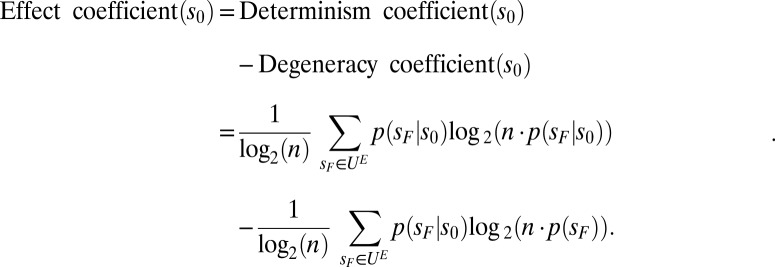
A state-independent informational measure of a system’s causal architecture can be obtained by taking the expected value of cause or effect information over all system states, a quantity called effective information (EI):

The two terms are identical, because the system is assumed to be time invariant (), and cause and effect information are related via Bayes’ rule. EI is also the mutual information (MI) between all possible causes and their effects, MI(U^C;U^E) (Effective Information EI(S) Expressed in Terms of Cause and Effect Information and Mutual Information MI).

As a measure of causation, EI captures how effectively (deterministically and uniquely) causes produce effects in the system, and how selectively causes can be identified from effects. As with the state-dependent measures, the effectiveness (Eff) of the causal interactions within a system can be captured by normalizing EI by the system’s size: 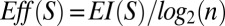. Also as in the state-independent case, effectiveness can be split into two components, determinism and degeneracy:

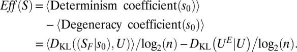Thus, Eff(S) = 1 if EI is maximal for a given system size, and decreases with indeterminism (divergence due to noise) or degeneracy (deterministic convergence), with Eff(S) = 0 for completely noisy or degenerate systems (Fig. 1 C and D). In a system with perfect effectiveness (Fig. 1B), each cause has a unique effect, and each effect has a unique cause. Thus, such a system [where Eff(S) = 1] is perfectly retrodictive/predictive, in the sense that not only the unique future trajectory, but also the unique past trajectory of all states can be deduced from the TPM (complete causal reversibility).

Levels of Analysis.

A finite, discrete system S can be considered at various levels, from the most fine-grained micro causal model S_m through various coarse-grained causal models S_M. All macro levels S_M are assumed to be “supervenient” on the micro level S_m: given the micro elements of S_m and the causal relationships between them, all other members of {S}—the set of all possible causal models of system S—are fixed as well (19). Although S_m fixes S_M, any S_M may be fixed by a number of different lower level descriptions, a property known as “multiple realizability” (20).

Groupings.

Micro elements are binary and labeled by Latin letters {A, B, C…}, macro elements by Greek letters {α, β, γ…}. Micro states are labeled {1, 0} and macro states {“on,” “bursting,” “quiet”…). Micro elements can be grouped into macro elements spatially, temporally, or both. Micro states are grouped into macro states through a mapping . The mapping must be exhaustive and disjunctive over micro elements (all of the states of one micro element must be mapped to the states of the same macro element; note that a macro element can consist of a single micro element as long as the state space of the system is reduced). Moreover, the mapping must be such that no micro-level information is available at the macro level (the identity of the micro elements grouped into a macro element is lost). For example, the grouping of the four states of two micro elements into the two states of one macro element as [[00, 01, 10] = off, [11] = on] is permitted, whereas the grouping [[00, 01], [10, 11]] is not, because distinguishing 01 from 10 requires knowing the identity of the micro elements.

Level-Specific Perturbations.

Causal analysis at the micro level S_m, requires setting S into all possible micro states with equal probability (i.e., testing all micro alternatives) and determining the resulting effects. When moving to a macro level S_M, S must similarly be set into all possible macro states with equal probability (i.e., testing all macro alternatives). To causally assess any macro state, then, one must set S into all of the n_micro micro states {s_m} that are grouped into the corresponding macro state s_M, and average over the effects. This is done using a “macro perturbation”: 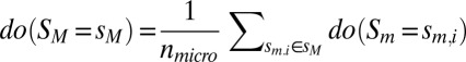. Using such macro perturbations, one can obtain cause/effect information and EI for every coarse grain of S_m. EI at each macro level is then equivalent to the MI between the set of macro causes and their macro effects.

Causal Emergence/Reduction.

Finally, by assessing EI(S) over all coarse grains of S_m, one can ask at which level of {S} causation reaches a maximum. This provides an analytical definition of causal emergence, expressed in bits: .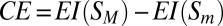

Thus, if EI(S) is maximal for a macro-level S_M rather than the micro-level S_m, then CE > 0 and causal emergence occurs. If for every macro-level CE < 0, causal reduction holds. Although the focus here is on emergence/reduction relative to the micro-level S_m, the above measure can of course be used to compare different macro levels.

As mentioned above, EI(S) depends on both the size of the system’s repertoire of states and on the effectiveness of its mechanisms. When moving from one system level to another, both terms change as the state space becomes smaller or larger, and the individual states become more or less selective with respect to the past, and more or less determined or degenerate with respect to the future. The respective informational contributions of repertoire size and effectiveness to ΔEI(S) can be expressed separately as follows: , where n_m/M is the state repertoire size of S_m/M. It follows that ΔEI = ∆I_Eff + ∆I_Size = CE. A positive ∆I_Eff can thus be due to the macro reducing the degeneracy of the micro level, increasing the determinism of the micro level, or both. Notably, coarse graining the micro-level S_m into macro-level S_M implies that ∆I_Size is always negative. Hence, for causal emergence to occur [EI(S_M) > EI(S_m)], the increase in effectiveness ∆I_Eff must outweigh the decrease in ∆I_Size.

Results

Causal analysis was performed across all coarse grains of a system [only the S_M with maximal EI(S) is shown in the figures] with a custom-made Python program. Data plots were created using MATLAB. Below, we consider examples of spatial, temporal, and spatiotemporal emergence (see Fig. S1 for an example of spatial reduction).

Spatial Causal Emergence.

As a proof-of-principle example, consider a system of four binary elements S_m = {ABCD} (Fig. 2A). Each micro mechanism is an AND-gate (two inputs) operating over some intrinsic noise. The 16 × 16 S_m TPM was constructed by setting the system into all possible micro states from [0000] to [1111] with equal probability (Fig. 2B). At the micro level S_m, effective information EI(S) = 1.15 bits, out of maximally 4 bits, with effectiveness Eff(S_m) = 0.29. The macro level S_M (Fig. 2D), composed of two elements {α, β}, each with states {“on,” “off”}, is a coarse graining of S_m as defined by the mapping M in Fig. 2C. The 4 × 4 S_M TPM was obtained by setting the system into all possible macro states from [off, off] to [on, on] with equal probability (Fig. 2E). For the macro level, EI(S_M) = 1.55 bits, higher than EI(S_m) = 1.15 bits. Thus, CE(S) = 0.40 bits, demonstrating that in this case the macro S_M beats the micro S_m and constitutes the optimal causal model of system S. This is because the TPM for S_M is much closer to perfect effectiveness [Eff(S_M) = 0.78] and the increase in effectiveness gained by grouping ∆I_Eff = 0.97 bits outweighs the loss in size ∆I_Size = −0.57 bits. In this example, the gain in effectiveness ∆I_Eff at the macro level comes primarily (91%) from counteracting noise [determinism coef. (S_m) = 0.34; (S_M) = 0.78] and less so (9%) from reducing degeneracy [degeneracy coef. (S_m) = 0.05; (S_M) = 0.006].

Fig. 2.

Spatial causal emergence (counteracting indeterminism). (A) The micro level S_m of system S is composed of identical noisy micro mechanisms. (B) The micro TPM. (C) A macro causal level S_M and its TPM are defined by the mapping M (shown for AB to α, CD to β is symmetric). (D) S_M and its macro mechanisms. (E) By reducing indeterminism and increasing effectiveness Eff, the macro beats the micro in terms of EI despite the reduced repertoire size (CE = 0.40 bits).

The higher effectiveness of the macro level is also evident comparing S_m and S_M in a state-dependent manner. As an example, the cause/effect distributions for S_m in state {ABCD} = [0001] are compared with the corresponding S_M state {αβ} = [off, off] in Fig. 3. Comparing the cause/effect distributions of S_m = [0001] against the unconstrained repertoires (using D_KL) yields 0.83 bits of cause information and 0.43 bits of effect information. For the macro S_M, cause information is 2 bits and effect information 1.35 bits. The macro beats the micro because {αβ} = [off, off] is both more selective and more reliable than {ABCD} = [0001].

Fig. 3.

State-dependent cause/effect information. (A) The cause information of S_m in micro state {ABCD} = [0001] is calculated as the difference (D_KL) between the cause repertoire of state [0001] and the unconstrained micro repertoire U^C (Left). The cause information of S_M in the supervening macro state {αβ} = [off/off] (Right) is the difference (D_KL), between the cause repertoire of [off/off] and the unconstrained macro repertoire U^C. (B) Effect information. The higher cause and effect information at the macro level is due to an increase in determinism and decrease in degeneracy, reflecting higher selectivity.

Causal emergence may arise not only from macro gains in determinism (as above), but also from reducing degeneracy. In Fig. 4, micro elements A–F are deterministic AND gates connected in a way that ensures high degeneracy (Fig. 4A, determinism coef. = 1; degeneracy coef. = 0.6), resulting in Eff(S_m) = 0.4 and EI(S_m) = 2.43 bits (Fig. 4C). The optimal macro groups the six micro AND gates into three macro COPY gates (αβγ) (Fig. 4B). Both macro and micro are deterministic, but by eliminating degeneracy ∆I_Eff = 1.79 bits > −∆I_Size = 1.22 bits. As a result, Eff(S_M) = 1, EI(S_M) = 3 bits, and the macro emerges over the micro (CE = 0.57 bits).

Fig. 4.

Spatial causal emergence (counteracting degeneracy). (A) A degenerate S_m with deterministic AND gates. (B) The cycle of AND gates is mapped onto a cycle of COPY gates at the macro level. (C) The deterministic but degenerate micro TPM. (D) The deterministic macro TPM with zero degeneracy. By eliminating degeneracy and achieving perfect effectiveness, the macro beats the micro (CE = 0.57 bits).

Temporal Causal Emergence.

The same principles allowing for emergence through spatial groupings hold for temporal groupings, which coarse grain micro time steps (t_x) into macro time steps (T_x). The example in Fig. 5 shows micro elements that, upon receiving an input “burst” of two spikes, respond with an output burst of two spikes. Thus, elements implement second-order Markov mechanisms over both inputs and outputs (Fig. 5A). Fig. 5B shows that causal interactions assessed over one micro time step are weak [EI(S_m) = 0.16 bits; Eff(S_m) = 0.03] because they fail to capture the second-order mechanisms. By contrast, causal analysis over two micro time steps (Fig. 5C) gives EI = 1.38 bits and Eff(S_m) = 0.34. The temporal grouping of micro into macro states α = {A_t, A_t+1} and β = {B_t, B_t+1} (Fig. 5D) is analogous to the spatial grouping in Fig. 2: {00, 01, 10} = {off} and {11} = {on}. Over macro time steps, the system becomes fully deterministic and nondegenerate, EI(S_M) = 2 bits, Eff(S_M) = 1, and CE(S) = 0.62 bits (Fig. 5 E and F).

Fig. 5.

Temporal causal emergence. (A) S_m is composed of second-order Markov mechanisms A and B: at t₀, each mechanism responds based on the inputs at t₋₂ and t₋₁, and outputs over t₀ and t₊₁. (B) Causal analysis over one micro time step gives an incomplete view of the system. (C) A causal analysis over two micro time steps reveals the second-order Markov mechanisms. (D) The optimal macro system S_M groups two micro time steps into one macro time step for macro elements {α,β}. (E) Each coarse grained macro mechanism effectively corresponds to a deterministic COPY gate. (F) The macro one-time step TPM S_M has Eff(S_M) = 1, and the micro two-time step TPM has Eff(S_m) = 0.34; CE = 0.62 bits.

Spatiotemporal Causal Emergence.

In general, emergence may occur simultaneously over space and time (Fig. 6). As in Fig. 5, the nine neural-like micro elements in Fig. 6A are second-order Markov mechanisms, integrating inputs and outputs over two micro time steps, t₋₂ t₋₁, and t₀ t₊₁, respectively [compare to longer time constants of NMDA receptors (21)]. Moreover, in the examples above, the micro elements within a macro element were not connected and were causally equivalent. To demonstrate that this is not a requisite for causal emergence, in Fig. 6, the micro elements are fully connected and causally heterogeneous (self-connections not drawn). All elements are spontaneously active (1) with heterogeneous probabilities: p(A/D/G) = 0.45; p(B/E/H) = 0.5; p(C/F/I) = 0.55. The elements are structured into three groups {ABC, DEF, GHI} due to different intragroup and intergroup mechanisms: within each group, if the sum of intragroup connections Σ(intra) = 0 (for two time steps), all elements stay 0 (for the next two time steps). However, if the sum of intergroup connections Σ(inter) = 6 from one or both of the other two groups over two time steps (burst of synchronous activity), p(1) is raised by 0.5 for the next two time steps (see Fig. S2 for macro and micro TPMs of a spatial system with equivalent rules). At the macro-level S_M (Fig. 6B), the three groups of neurons become macro elements, and two micro time steps (t_x) are grouped into one macro time step (T_x). In neural terms, these macro elements could represent “minicolumns” having three states: “inhibited” (all minicolumn neurons silent at T_x), “receptive” (some firing at T_x), or “bursting” (all firing at T_x). Macro causal interactions can be summarized as follows: if a macro element is inhibited, only receiving a burst can move it to the receptive or (more unlikely) the bursting state; otherwise, it stays inhibited. As in previous examples, the coarse-grained S_M has higher EI(S_M) = 3.51 bits and Eff(S_M) = 0.74 than S_m [EI(S_m) = 0.59 bits; Eff(S_m) = 0.033]. In this case, spatiotemporal causal emergence [CE(S) = 2.92 bits] is due to an increase in determinism that far outweighs a slight increase in degeneracy and the decrease in size.

Fig. 6.

Spatiotemporal causal emergence. (A) A “neuronal” system merging the temporal characteristics of the system in Fig. 5 with a differentiated spatial structure (Fig. S2). Regular and rounded arrows indicate intergroup and intragroup connections, respectively. (B) Each macro element receives inputs from itself and the other macro element. The macro level beats the micro level, leading to spatiotemporal emergence [CE(S) = 2.92 bits].

Discussion

This paper provides a principled way of assessing at which spatiotemporal grain size the causal interactions within a system reach a maximum. Causal interactions are evaluated by effective information (EI), a measure that is sensitive both to the effectiveness of the system’s mechanisms and to the size of its state space. Examples with simulated systems demonstrate that, after coarse graining the micro mechanisms in both space and time, EI can be higher at a macro level than at a micro level. In these cases, the macro mechanisms, rather than the micro ones, can be said to be doing the causal work within a system.

Effective Information, Effectiveness, and Emergence.

As shown here, EI corresponds to the “effectiveness” of a system’s mechanisms multiplied by repertoire size, expressed in bits. Effectiveness Eff(S) is the average of the effect coefficients over all system states. The effect coefficient measures to what extent the current system state is necessary to specify the system’s future state. This, in turn, is a function of determinism minus degeneracy. On the cause side, the equivalent to the effect coefficient is the cause coefficient, which measures to what extent the current state is sufficient to specify the system’s past state. For a particular current state, cause and effect coefficients may differ: for example, a state may have many causes but only one effect. However, the average of the effect coefficients over system states, i.e., effectiveness, corresponds to the average of the cause coefficients (weighted by the probability of the effects). In other words, within a time-invariant system the average selectivity of the causes corresponds to the average selectivity of the effects. Note that, in principle, other measures of causation that, like EI, reflect causal structure (selectivity, determinism, degeneracy) and system size, should demonstrate causal emergence as well.

The main result obtained in the simulations is that coarse graining, both in space and in time, can yield a higher value of EI. This happens even though the micro has, by definition, a larger state space than the macro—an advantage with respect to EI. Given this inherent advantage of the micro, it is understandable why the default scientific strategy for analyzing systems has been one of reduction (Causal Reduction). However, the examples presented above show that the inherent loss in EI due to the macro’s smaller repertoire size can be offset if the macro achieves a greater gain in effectiveness. In turn, greater effectiveness stems from macro mechanisms constructed from their constituting micro mechanisms in such a way that, at the macro level, determinism is increased and/or degeneracy is decreased. Genuine causal emergence can then be said to occur whenever there is a gain in EI (CE > 0) at the optimal macro level. If instead there is a loss in EI (CE < 0), causal reduction is appropriate, and the micro level is the optimal level of causal analysis. The causal approach pursued here suggests that qualitative or noncausal accounts of emergence may have been hindered by not being able to characterize how and why a macro level can actually have greater causal effectiveness than a micro level (22, 23).

Micro Macro Mappings and Repertoires of Alternatives.

The present approach makes it possible to compare causation at the micro and macro levels in a fair manner. First, the simulated examples are such that the macro supervenes strictly upon the micro: once the micro is defined, all macro levels are fixed. Specifically, no extra causal ingredients are added at the macro level, such as rules that apply to the macro only (24). Furthermore, the mapping of micro into macro elements is such that the identity of micro elements is lost; otherwise, the macro level would have access to micro-level information that could offset its reduced repertoire size. Finally, when causation is evaluated a uniform distribution of alternatives is imposed independently at the micro and macro levels. For this uniform distribution of perturbations to be imposed at the macro level, the probability of the underlying micro perturbations must be modified by averaging the micro states that map into the same macro state. The modified distribution of micro perturbations yielding a uniform distribution of macro perturbations makes EI sensitive to the causal structure at each level, ultimately allowing the supervening macro EI to exceed the micro EI.

Emergence as an Intrinsic Property of a System.

EI is a causal measure, because it requires perturbing the system in all possible ways and evaluating the resulting effects on the system. It is also an informational measure, because its value depends on the size of the repertoire of alternatives. Indeed, in the present approach, causation and information are necessarily linked (25), hence the term “effective information.” Finally, measuring EI reveals an “intrinsic” property of the system, namely the average effectiveness/selectivity of all possible system states with respect to the system itself. Effectiveness/selectivity can be assessed at multiple spatiotemporal grains, and the particular spatiotemporal grain at which EI reaches a maximum is again an intrinsic property of the system. This in no way precludes an observer from profitably investigating the system’s properties at other macro levels, at the micro level, or at multiple levels at once (e.g., neuroscientists studying the brain at the level of ion channels, individual neurons, local field potentials, or functional magnetic resonance signals). However, causal emergence implies that the macro level with highest EI is the one that is optimal to characterize, predict, and retrodict the behavior of the system—the one that “carves nature at its joints” (26).

The search for the macro level at which EI is maximal has a parallel in information theory: channel capacity is an intrinsic property defined as the maximal amount of information that can be transmitted along the channel at a certain rate, found by searching over all possible input distributions (27). Finding the optimal level of coarse graining for causal emergence is based on a similar search, with several differences. First, EI is evaluated using perturbations over the system itself, rather than across a channel (the system is its own input and output). Second, the probability distributions over micro states that can be considered must conform to a proper mapping of micro into macro elements (or time intervals). Additional connections of causal emergence to established measures, such as reversibility and lumping in Markov processes (28), or epsilon machines (29), are a potential subject for future work.

Causal Exclusion and Its Implications.

Causal analysis as presented here endorses both supervenience (no extra causal ingredients at the macro level) and causal exclusion [for a given system at a given time, causation occurs at one level only, otherwise causes would be double counted (4)]. However, causal analysis also demonstrates that EI can actually be maximal at a macro level, depending on the system’s architecture. In such cases, causal exclusion turns the reductionist assumption on its head, because to avoid double-counting causes, optimal macro causation must exclude micro causation. In other words, macro mechanisms can always be decomposed to their constituting micro mechanisms (supervenience); however, if there is emergence, macro causation does not reduce to micro causation, in which case the macro wins causally against the micro and takes its place (supersedence). The notion of irreducibility among levels (does the macro beat the micro?) is complemented by the notion of irreducibility among subsets of elements within a level [is the whole more than its parts (15, 25)?]. From the perspective of a system, emergence (CE > 0) implies causal “self-definition” at the optimal macro level—the one at which its causal interactions “come into focus” (30) and “the action happens.”

Applicability to Real Systems.

Measuring EI exhaustively, across all micro/macro levels, is not feasible for complex physical or biological systems (Applicability—Network Motifs as Indicators of Emergence). However, some useful guidelines can be derived from the above analysis: (i) if Eff(S_m) ≥ Eff(S_M), then causal emergence is impossible and causal reduction holds; (ii) if EI(S_m) > log₂(n_M), where n_M is the state repertoire size of S_M, causal reduction holds; (iii) if for some coarse graining, Eff increases drastically, causal emergence is to be suspected (as ∆I_Eff >> −∆I_Size). Therefore, systems that already are close to maximal effectiveness at the micro level (Fig. S1) indicate causal reduction. By contrast, heavily interconnected groups of elements with spontaneous activity and the ability to distinguish between intragroup and intergroup connections, such as the simplified neural system of Fig. 6, are more suitable for emergence.

In real neural systems, one could compare the respective effective information at the micro scale of single neurons over millisecond intervals, the meso scale of neuronal groups over hundreds of milliseconds, and the macro scale of brain regions over several seconds (using tools such as optogenetics and calcium imaging). In this way, classic notions, such that cortical minicolumns may constitute the fundamental units of brain function (31), or that the cortex works by population coding in space (32) or rate coding in time (33) in the face of high intertrial variability (34), could then be tested rigorously using a measure of effectiveness. Examining small motifs that are overrepresented in complex networks [such as brains (35)] could determine whether the network as a whole is biased toward emergence or reduction. Heuristic assessments of the likelihood of emergence could also rely on the analysis of wiring diagrams, which can offer an estimate of degeneracy, combined with knowledge of the amount of intrinsic noise in a system, which can provide an estimate of determinism.

Conclusions

The approach to emergence investigated here provides theoretical support for the intuitive idea that, to find out how a system works, one should find the “differences that make [most of] a difference” to the system itself (25) (cf. ref. 36). It also suggests that complex, multilevel systems such as brains are likely to “work” at a macro level because, in biological systems, selectional processes must deal with unpredictability and lead to degeneracy (18). This may also apply to some engineered systems designed to compensate for noise and degeneracy. More broadly, this view of causal emergence suggests that the hierarchy of the sciences, from microphysics to macroeconomics, may not just be a matter of convenience but a genuine reflection of causal gains at the relevant levels of organization.

References

- 1.Sporns O, Tononi G, Kötter R. The human connectome: A structural description of the human brain. PLoS Comput Biol. 2005;1(4):e42. doi: 10.1371/journal.pcbi.0010042. [DOI] [PMC free article] [PubMed] [Google Scholar]
- 2.Markram H. The blue brain project. Nat Rev Neurosci. 2006;7(2):153–160. doi: 10.1038/nrn1848. [DOI] [PubMed] [Google Scholar]
- 3.Davidson D. Mental events. In: Block N, editor. Readings in Philosophy of Psychology. Vol 1. Cambridge, MA: Harvard Univ Press; 1980. pp. 107–119. [Google Scholar]
- 4.Kim J. Supervenience and Mind: Selected Philosophical Essays. Cambridge, UK: Cambridge Univ Press; 1993. [Google Scholar]
- 5.Kim J. Mind in a Physical World: An Essay on the Mind-Body Problem and Mental Causation. Cambridge, MA: MIT Press; 2000. [Google Scholar]
- 6.Bontly T. The supervenience argument generalizes. Philos Stud. 2002;109:75–96. [Google Scholar]
- 7.Seth A. Measuring emergence via nonlinear Granger causality. ALIFE. 2008;2008:545–552. [Google Scholar]
- 8.Hölldobler B, Wilson E. The Superorganism: The Beauty, Elegance, and Strangeness of Insect Societies. New York: W. W. Norton; 2009. [Google Scholar]
- 9.Sperry R. Science and Moral Priority: Merging Mind, Brain, and Human Values. New York: Columbia Univ Press; 1983. [Google Scholar]
- 10.Sawyer R. Social Emergence: Societies as Complex Systems. Cambridge, UK: Cambridge Univ Press; 2005. [Google Scholar]
- 11.Broad C. The Mind and Its Place in Nature. London: Routledge & Kegan Paul; 1925. [Google Scholar]
- 12.Bar‐Yam Y. A mathematical theory of strong emergence using multiscale variety. Complexity. 2004;9:15–24. [Google Scholar]
- 13.Tononi G, Sporns O. Measuring information integration. BMC Neurosci. 2003;4:31. doi: 10.1186/1471-2202-4-31. [DOI] [PMC free article] [PubMed] [Google Scholar]
- 14.Pearl J. Causality: Models, Reasoning and Inference. Cambridge, UK: Cambridge Univ Press; 2000. [Google Scholar]
- 15. Albantakis L, Hoel EP, Koch C, Tononi G (2013) Intrinsic Causation and Consciousness. Association for the scientific study of consciousness conference (ASSC17). Available at www.theassc.org/files/assc/docs/ASSC17-PB-070113-online-version-with-Addendum.pdf. Accessed November 2, 2013.
- 16.Kullback S. Information Theory and Statistics. New York: Dover Publications; 1997. [Google Scholar]
- 17.Edelman GM. Neural Darwinism: The Theory of Neuronal Group Selection. New York: Basic Books; 1987. [DOI] [PubMed] [Google Scholar]
- 18.Tononi G, Sporns O, Edelman GM. Measures of degeneracy and redundancy in biological networks. Proc Natl Acad Sci USA. 1999;96(6):3257–3262. doi: 10.1073/pnas.96.6.3257. [DOI] [PMC free article] [PubMed] [Google Scholar]
- 19.Stalnaker R. Varieties of supervenience. Philos Perspect. 1996;10:221–241. [Google Scholar]
- 20.Fodor J. Special sciences (or: The disunity of science as a working hypothesis) Synthese. 1974;28:97–115. [Google Scholar]
- 21.Jahr CE, Stevens CF. Voltage dependence of NMDA-activated macroscopic conductances predicted by single-channel kinetics. J Neurosci. 1990;10(9):3178–3182. doi: 10.1523/JNEUROSCI.10-09-03178.1990. [DOI] [PMC free article] [PubMed] [Google Scholar]
- 22.Bedau M. Weak emergence. Noûs. 1997;31:375–399. [Google Scholar]
- 23.Chalmers D. Strong and weak emergence. In: Clayton P, Davies P, editors. The Reemergence of Emergence. Oxford: Oxford Univ Press; 2006. pp. 244–256. [Google Scholar]
- 24.Butterfield J. Laws, causation and dynamics at different levels. Interface Focus. 2012;2(1):101–114. doi: 10.1098/rsfs.2011.0052. [DOI] [PMC free article] [PubMed] [Google Scholar]
- 25.Tononi G. Integrated information theory of consciousness: An updated account. Arch Ital Biol. 2012;150(2-3):56–90. doi: 10.4449/aib.v149i5.1388. [DOI] [PubMed] [Google Scholar]
- 26.Hamilton E, Cairns H. The Collected Dialogues of Plato: Including the Letters. New York: Pantheon Books; 1961. [Google Scholar]
- 27.Shannon CE. The mathematical theory of communication. 1963. MD Comput. 1997;14(4):306–317. [PubMed] [Google Scholar]
- 28.Kemeny J, Snell J. Finite Markov Chains. New York: Springer; 1976. [Google Scholar]
- 29.Shalizi C, Crutchfield J. Computational mechanics: Pattern and prediction, structure and simplicity. J Stat Phys. 2001;104:817–879. [Google Scholar]
- 30.Alexander S. Space, Time, and Deity: The Gifford Lectures at Glasgow, 1916–1918. London: Macmillan; 1920. [Google Scholar]
- 31.Buxhoeveden DP, Casanova MF. The minicolumn hypothesis in neuroscience. Brain. 2002;125(Pt 5):935–951. doi: 10.1093/brain/awf110. [DOI] [PubMed] [Google Scholar]
- 32.Georgopoulos AP, Schwartz AB, Kettner RE. Neuronal population coding of movement direction. Science. 1986;233(4771):1416–1419. doi: 10.1126/science.3749885. [DOI] [PubMed] [Google Scholar]
- 33.London M, Roth A, Beeren L, Häusser M, Latham PE. Sensitivity to perturbations in vivo implies high noise and suggests rate coding in cortex. Nature. 2010;466(7302):123–127. doi: 10.1038/nature09086. [DOI] [PMC free article] [PubMed] [Google Scholar]
- 34.Knoblauch A, Palm G. What is signal and what is noise in the brain? Biosystems. 2005;79(1-3):83–90. doi: 10.1016/j.biosystems.2004.09.007. [DOI] [PubMed] [Google Scholar]
- 35.Sporns O. Networks of the Brain. Cambridge, MA: MIT Press; 2010. [Google Scholar]
- 36.Fitelson B, Hitchcock C. Probabilistic Measures of Causal Strength. Oxford, UK: Oxford Univ Press; 2010. [Google Scholar]
Associated Data
This section collects any data citations, data availability statements, or supplementary materials included in this article.