Image regions contributing to perceptual translucency: A psychophysical reverse-correlation study

Abstract

The spatial luminance relationship between shading patterns and specular highlight is suggested to be a cue for perceptual translucency (Motoyoshi, 2010). Although local image features are also important for translucency perception (Fleming & Bulthoff, 2005), they have rarely been investigated. Here, we aimed to extract spatial regions related to translucency perception from computer graphics (CG) images of objects using a psychophysical reverse-correlation method. From many trials in which the observer compared the perceptual translucency of two CG images, we obtained translucency-related patterns showing which image regions were related to perceptual translucency judgments. An analysis of the luminance statistics calculated within these image regions showed that (1) the global rms contrast within an entire CG image was not related to perceptual translucency and (2) the local mean luminance of specific image regions within the CG images correlated well with perceptual translucency. However, the image regions contributing to perceptual translucency differed greatly between observers. These results suggest that perceptual translucency does not rely on global luminance statistics such as global rms contrast, but rather depends on local image features within specific image regions. There may be some “hot spots” effective for perceptual translucency, although which of many hot spots are used in judging translucency may be observer dependent.

1. Introduction

Translucency (and transparency) is a typical feature of the material surface qualities of objects obtained through visual information. Many studies have focused on the stimulus conditions that yield perceptual transparency, as shown in Metelli's theory (Metelli, 1974; Singh & Anderson, 2002). These studies have employed flat, simple, two-dimensional (2D) stimuli composed of several spatial patches with different luminances or colors. They claimed that the luminance (and color) relationship between spatial regions in such a stimulus is an important factor determining whether the stimulus can induce transparency perception, that is, perception of a transparent filter on a background-textured surface. Indeed, this type of model can predict perceptual transparency of a simple flat stimulus well with only several planes with different luminances and colors as used in these studies.

However, this type of model can be applied only to perceptual transparency in limited situations in daily life. Many everyday objects, such as glass, plastics, skin, and waxes, produce translucent and transparent perception. The optical characteristics of these translucent and transparent materials are quite complicated. Not only the transmittance but also the subsurface scattering of these objects, which is scattering of incident light under object surfaces, contributes to perceptual translucency and transparency, as shown in the fact that parameters associated with these optical phenomenon models are prepared in typical computer graphics (CG) software (Jensen & Buhler, 2002). The models that predict perceptual transparency described above, such as Metelli's theory, cannot clearly predict the perceptual translucency and transparency of real 3D objects with such complicated optical factors. The reason is that we can perceive the translucency of these objects even without background images shown through them, whereas Metelli's theory assumes that background texture can be seen through a transparent object (Singh & Anderson, 2002).

What types of image processing can predict perceptual translucency and transparency in images of 3D objects that have transmittance or subsurface scattering? One approach is inverse rendering of the images, which is used in some computer vision studies (e.g., Boivin & Gagalowicz, 2001; Ramamoorthi & Hanrahan, 2001). Images (or retinal images) of objects are created on the basis of combinations of light fields (illumination environment), object shapes, and the surface qualities (materials) of objects. The inverse rendering approaches used in engineering typically estimate one of these three factors, such as the surface reflectance or illumination directions, under conditions where the other two factors are given (Boivin & Gagalowicz, 2001; Ramamoorthi & Hanrahan, 2001). However, because our visual system rarely knows the physical parameters of the three factors, the inverse rendering approach used in the engineering field seems quite implausible as a strategy for the visual system to estimate surface qualities including transmittance and subsurface scattering, although some human psychophysical studies of color constancy suggested that human observers can estimate color of light illuminating a scene from a single view for a single light source scene (see Foster, 2011, for a review).

It was suggested recently that the visual system may employ simpler strategies than the inverse rendering approach to estimate surface qualities on the basis of image features such as simple image statistics. For example, the luminance skewness of object images may be an important cue for estimating the perceptual glossiness of 3D objects (Motoyoshi, Nishida, Sharan, & Adelson, 2007; Sharan, Li, Motoyoshi, Nishida, & Adelson, 2008, but see Anderson & Kim, 2009; Kim, Marlow, & Anderson, 2011; Marlow, Kim, & Anderson, 2012). Similarly, regarding perceptual translucency and transparency, Motoyoshi (2010) suggested, from simple psychophysical experiments using stimuli made with CG software, that image features based on an entire object image, such as contrast and the spatial relationship between specular highlights and the non-specular components of glossy objects, can be a robust cue for perceptual translucency. He also demonstrated that controlling the rms contrast of low spatial frequency components of the entire image luminance could alter the perceptual translucency, which suggests the effectiveness of these cues. Fleming and Bulthoff (2005) suggested a similar importance of the luminance contrast or luminance histogram for perceptual translucency.

Here, we question whether image features based on an entire image region are an important cue for perceptual translucency. The luminance or luminance contrasts of the edges or corners in an object image have been suggested to be much more important than luminance information for the other regions in an object image (Fleming & Bulthoff, 2005). Considering this suggestion, certain local regions within an object image may have other stronger cues for perceptual translucency than others. Psychophysical reverse-correlation methods such as the classification image method (Ahumada, 1996; Murray, 2011) have recently been used to investigate the spatial regions of visual stimuli that were important for different types of visual tasks. For example, image regions within human faces that contribute to face category identification have been extracted by psychophysical reverse-correlation methods (Mangini & Biederman, 2004; Nestor & Tarr, 2008). In this study, we extract the regions in CG images that are strongly related to perceptual translucency. An analysis of the luminance properties of these regions, once they are extracted, may provide us with knowledge about image features that the human visual system employs to perceive the translucency of objects.

2. Methods

2.1. Observers

Seven observers (two females and five males, mean age of 24.4 years) with normal or corrected-to-normal visual acuity participated in our experiments. Written informed consent forms were collected from all the observers in accordance with the rules defined by the Committee for Human Research of Toyohashi University of Technology.

2.2. Apparatus

The stimuli were displayed on a CRT monitor (TOTOKU CV722X, 1024 × 768 pixels, 60 Hz) connected to a graphics card (NVDIA GeForce GTS 400) on a personal computer (Dell Vostro 430 with Core i5 750 and 3 GB of RAM). PsychToolbox (Brainard, 1997) on MATLAB (MathWorks) controlled the experimental sequences. The luminance of the monitor was measured with Cambridge Research Systems ColorCAL2 to calculate the stimulus luminance statistics in the following sections. The observer's head was roughly fixed with a chin rest. The observer viewed the stimuli binocularly at a distance of 57 cm from the CRT screen.

2.3. Stimuli

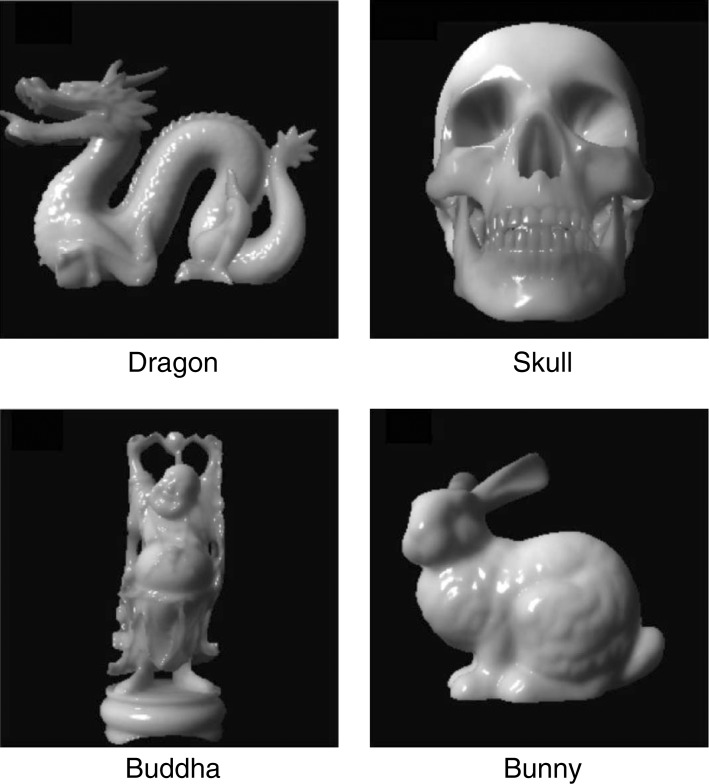
We used the CG software LightWave ver. 9.6 to create the stimulus images. We used four stimulus objects having the 3D shapes shown in Figure 1: Dragon, Buddha, and Bunny from the Stanford 3D Scanning Repository (http://graphics.stanford.edu/data/3Dscanrep/), and Skull from the LightWave Object content. The size of the rendered image squares, including the black background, was 256 × 256 pixels (7.8 deg × 7.8 deg).

Figure 1.

Image samples of four shapes used in experiments.

The sizes and positions of objects in the 3D scenes in the CG images were defined in the LightWave coordinate system consisting of the X, Y, and Z axes. The sizes of the 3D objects varied somewhat with the object shape, but (X, Y, Z) was approximately (7, 7, 7 m) [e.g., the actual size of skull was (X, Y, Z) = (7, 6, 9 m)], and their center positions were (X, Y, Z) = (0, 0, 0 m). The illumination in the scene was a single point light source positioned at (X, Y, Z) = (−10, 10, −10 m) and facing the center of the object. The viewing camera was positioned at (X, Y, Z) = (0, 28.5, −14 m). There was no ambient illumination around the object. Here, the sizes of the objects in the 3D scenes seem quite large. In addition, perceptual translucency has been known to decrease as object sizes increase if the optical properties of the objects are fixed (Fleming & Bulthoff, 2005). However, the scales of the stimulus sizes are of course arbitrary units, and the effects of sizes on translucency perception can be compensated for by scaling both of the object size and the translucency parameter distance, which is described below.

The parameters regarding the surface qualities other than those directly related to translucency perception were fixed. Diffuse was set to 100%, specularity was 100%, glossiness was 60%, transparency was 0%, and refraction index was 1.4. The SSS2 algorithm in the software emulated the effects of subsurface scattering on the luminance profiles of the CG image objects, producing perceptual translucency. The distance parameter in the SSS2 function controlled the strength of the subsurface scattering. The rendered images of the objects were converted into 8-bit bitmap images. A previous study confirmed that the distance parameter controlled the perceptual translucency well (Motoyoshi, 2010). We also asked observers to compare the perceptual translucency of images with different distance values and confirmed that larger distance values facilitated translucency perception.

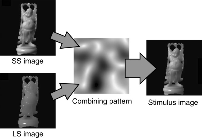
We employed a psychophysical reverse-correlation method to extract image regions that correlated well with perceptual translucency, as described in Section 1. To provide the random differences in the CG images that are needed in reverse-correlation methods, two CG images with different distance parameters were combined using a combining pattern that determined the randomness of the combined image. The combining pattern, shown in the center of Figure 2, was created by applying a low-pass Gaussian filter (standard deviation was 15 pixels) to a white-noise image of 256 × 256 pixels, and by normalizing the values from 0 to 1. The distance parameters of the two images used for the combination were (1 × x) m and (10 × x) m, in which x was different in each trial. The image with a distance of (10 × x) m seemed more translucent than that with (1 × x) m because of its stronger subsurface scattering, as shown on the left in Figure 2. Here, the less translucent image was referred to as a small subsurface scattering (small-scattering) image, and the more translucent one as a large subsurface scattering (large-scattering) image. In our rendering situations, the mean luminances within the object region of the large-scattering images were lower than those of the corresponding small-scattering images because some of the light incident upon the front surfaces of a large-scattering object was emitted even from the back of the object owing to the large subsurface scattering effects. This rule regarding the mean luminance, of course, does not apply to general cases, especially where light sources exist behind a target object, as in global illumination maps (Debevec, 1998). In addition, the rms contrasts in the object regions of the large-scattering images were lower than those of the corresponding small-scattering images, as shown in previous studies (Fleming & Bulthoff, 2005; Motoyoshi, 2010). Here, we refer to the luminance of pixel I of a small-scattering image as L_1i and to that of a pixel of a large-scattering image as L_10i. In addition, we refer to the value of the combining pattern of pixel i as C_i. Then, the luminance of pixel i in the combined image, L_ci, is calculated as

$${\displaystyle L_{\mathit{ci}}=L_{1i}{C}_i+L_{10i}(1-C_i).}$$

That is, C_i determines the ratio of the luminances in each pixel of a large-scattering image and a small-scattering image. For example, because the whitish regions in the combining pattern in Figure 2 have values near 1, these regions of the combined image based on this combining pattern should contain more of the luminance components of the large-scattering image, and those in blackish regions should contain more of the luminance components of the small-scattering image. The mean value of each combining pattern was set to 0.5 to roughly balance the large- and small-scattering image luminance components in the single combined image, although the mean values of the combining patterns within object regions other than the black background regions were not strictly controlled. Figure 3(a) shows five combined images based on different combining patterns. The reader may find slight differences in perceptual translucency among these five images. If that is the case, the relationship between the perceptual translucency and combining patterns can provide information about which image regions are dominant for translucency judgments by observers.

Figure 2.

Schematic of stimulus creation based on combining pattern. Luminances of a small-scattering image (distance was 1 + x m) and a large-scattering image (distance was 10 + x m) were combined on the basis of a combining pattern.

Figure 3.

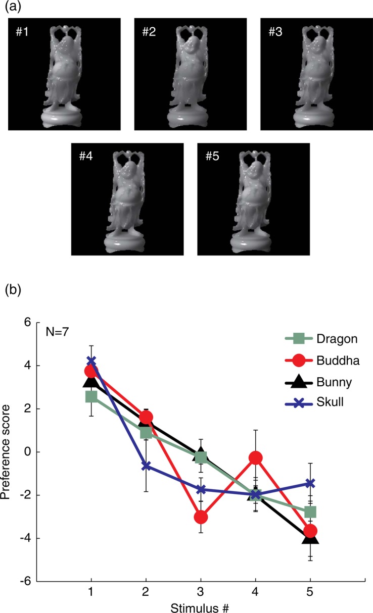
(a) Five Buddha images created using different combining patterns. The number shown in each image (which was not shown in the actual stimuli) indicates the stimulus number in the pre-experiment. (b) Results of pre-experiment. The abscissa shows the stimulus number shown in Figure 3(a), and the ordinate shows the preference score in relative translucency judgments measured in the pre-experiment. Larger preference scores correspond to judgments of greater translucency.

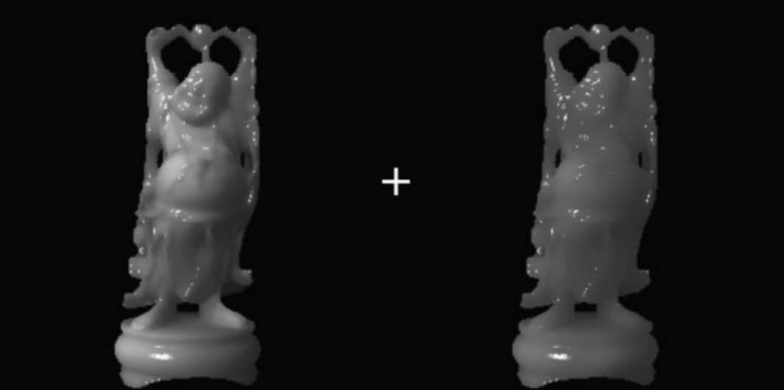
In the main experiment, two images created using different combining patterns were presented simultaneously to the left and right of a fixation cross at the center of the display (0.3 deg × 0.3 deg, 86.3 cd/m²), as shown in Figure 4. There was no gap between the left and right images, although the object regions do not seem to border each other because they were surrounded by black background regions.

Figure 4.

Example of stimulus used in the main experiment. Two images created from different combining patterns were simultaneously presented to the right and left of a white fixation cross at the center of the screen.

2.4. Pre-experiment

Before the main experiment, we had to confirm whether the random combining patterns were able to alter the perceptual translucency, and if the observer could judge relative differences in perceptual translucency between combined images created using different combining patterns. These questions were crucial for the reverse-correlation approach used in our experiment. To investigate this issue, we prepared five combined images using different combining patterns for each objects. The used combining patterns were different between the objects (e.g., Figure 3a shows images based on combining patterns only for Buddha). These five images were selected from many combined images so that an observer YO (one of the authors) felt that the variations in perceptual translucency were large for each object shape. The image numbers shown in Figure 3(a) were assigned on the basis of the strength of perceptual translucency reported by YO. Image numbers were also assigned for the other object shapes in the same way.

We adopted a paired comparison procedure to measure the relative perceptual translucency between these five images. In a trial in the pre-experiment, two of the five images were presented simultaneously for 1 s as shown in Figure 4. After the stimulus presentation, the observer judged which of the two images was more translucent and pressed a mouse button corresponding to this judgment. There were ₅C₂ = 10 image pairs, and each observer responded 10 times per image pair. All trials were included in a single session, and the order of image pairs in a session was randomized for each observer. We calculated the preference scores for all five images according to Thurstone's standard procedure.

Figure 3(b) shows the measured preference scores averaged across the observers. The preference scores clearly showed monotonically decreasing trends, suggesting that the combining patterns produced differences in perceptual translucency and the observers were able to judge these relative translucency differences. Thus, we confirmed that the combining pattern can be employed as a random factor to manipulate the perceptual translucency.

2.5. Procedures

In a trial in the main experiment, two images were presented simultaneously for 1 s with a central fixation point, as shown in Figure 4. The parameter x of either of the two images was 0, and that of the other was a positive value controlled by a staircase procedure. After the stimulus presentation, the observer judged which of the two images seemed to be more translucent and pressed a mouse button corresponding to this judgment. The difficulty of the task was controlled using a 1-up 2-down staircase procedure by adjusting the parameter x. Larger x values yielded larger distance values in an image as a whole, leading to stronger translucency perception. Therefore, large x values yielded strong response biases such that the image with non-zero x tended to be judged as more translucent. In this sense, x can be considered as a type of signal in the judgment of perceptual translucency. In addition, the differences between combining patterns should affect the perceptual translucency independently of x, as demonstrated in the results of the pre-experiment. In that regard, the combining patterns can be considered as a type of noise in the translucency judgment. A single session included two staircases, one that started from x = 0 and another that started from a large x value, for each of the four object shapes. Because each staircase terminated after 50 trials, a session consisted of 8 × 50 = 400 trials. Each observer participated in 30 sessions in total, resulting in 3,000 trials per object shape. Combining images were randomly generated for each trial, leading to different 3,000 combining pattern pairs per object shape.

3. Results

3.1. Basic analysis

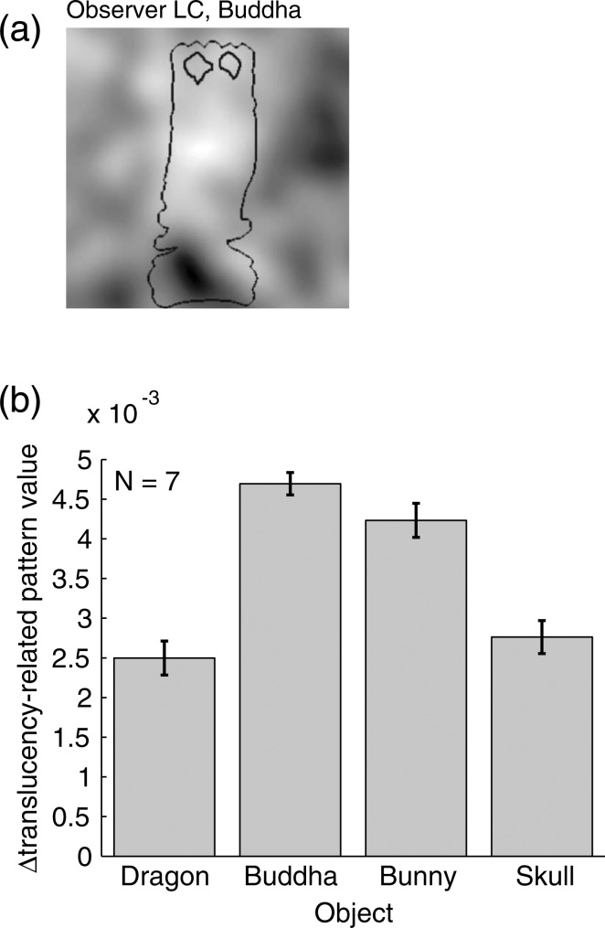
We analyzed the results using a method similar to standard classification image analysis (Ahumada, 1996; Gold, Murray, Bennett, & Sekuler, 2000) as follows. First, the two combined images in each trial were divided into two classes, more translucent and less translucent, on the basis of the observer's response for the trial. Then the combining patterns belonging to each class were averaged across all trials within each observer. Finally, the averaged pattern of the less translucent class was subtracted from that of the more translucent class. We refer to this resulting pattern as the “translucency-related pattern.” An example of translucency-related patterns is shown in Figure 5(a) with a contour of an object region.

Figure 5.

(a) Example of translucency-related pattern derived from an observer. Black line represents the contour of the object shape. (b) Difference between translucency-related pattern values within the object contour and outside of the contour (values within contour values outside of contour).

The mean values of the translucency-related patterns were zero for all object shapes, since the translucency-related patterns were accumulations of differences of the combining patterns with an identical mean value of 0.5. However, the mean values of the translucency-related patterns calculated only within the object contours were not zero. Indeed, the spatial regions within the object contours in the translucency-related patterns looked whiter than the regions outside the object contours (e.g., Figure 5a). The differences between the averaged values of the translucency-related patterns within and outside the object regions are shown in Figure 5(b). Unsurprisingly, the values are significantly greater than zero; that is, the values of the translucency-related patterns within the object regions are higher than those outside the object regions, suggesting that the observers perceived the objects as more translucent when the combining patterns offered more of the luminance components of the large-scattering images than those of the small-scattering images. Thus, we converted the translucency-related patterns into modified translucency-related patterns in a simple way. First, the average value of each translucency-related pattern within the object region was calculated. This value represents how much more luminance components of a large-scattering image were included in the object region of a stimulus corresponding to a “more translucent” response than that of a small-scattering image. Second, the average value was subtracted from its translucency-related pattern. With this procedure the mean value in the object region of this modified pattern became zero. Namely, a combined image created on the basis of this pattern as a combining pattern had equal amounts of luminance components of a large- and a small-scattering image. This modified pattern was referred to as “modified translucency-related pattern.” We introduced this definition of the modified translucency-related pattern in order to focus on just the spatial properties of the translucency-related patterns, not the effects of the relative amounts of the luminance components of the large- and small-scattering images. In the analysis below, we sometimes utilize these modified translucency-related patterns instead of the original translucency-related patterns.

3.2. Effects of translucency-related patterns on perceptual translucency

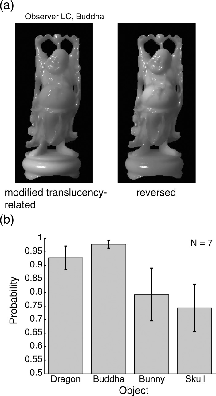
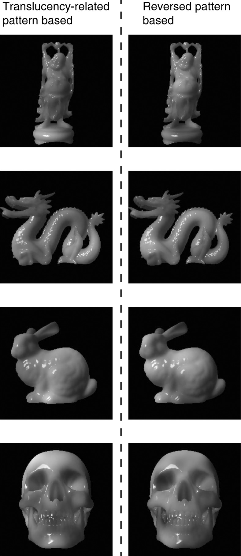
First, we confirm that the translucency-related patterns (especially the modified translucency-related patterns, which contained only the effects of the spatial distributions of the luminance components of the large- and small-scattering images) contained information about the strategy of the observer to judge translucency. A combining pattern can be derived simply by normalizing a modified translucency-related pattern into a range from 0 to 1 while keeping the mean value at 0.5. A combined image created from this result-based combining pattern should be able to induce strong translucent perception if the modified translucency-related pattern contained information useful for translucency judgment. In contrast, normalizing a reversed modified translucency-related pattern (that is, reversing the sign of the modified translucency-related pattern) produces another combining pattern, which should induce weak translucent perception. Therefore, we created two combined stimuli: one was based on a combining pattern from a modified translucency-related pattern and the other was based on another combining pattern from a reversed modified translucency-related pattern. These stimuli are shown in Figure 6(a). We presented these two images simultaneously on the monitor as in the main experiment, and asked the observer to judge which one seemed more translucent. The observer performed the task against the images created using her or his own modified translucency-related patterns in order to consider the effects of individual differences in the translucency-related patterns. We collected 20 trials for each object shape and observer.

Figure 6.

(a) Images based on modified translucency-related pattern (see the text) and reversed modified translucency-related pattern. (b) Probability that observers reported that the image based on the modified translucency-related pattern was more translucent than that based on the reversed pattern for each object shape. These probabilities are averaged across the observers.

The rates of trials in which the image based on the modified translucency-related patterns seemed more translucent are shown in Figure 6(b). The rates are significantly higher than the chance level (0.5) for all of the object shapes, indicating that the modified translucency-related patterns (and of course the translucency-related patterns) surely reflect the spatial profile of the regions affecting the observer's judgment of perceptual translucency. Thus, we analyze the spatial profile of the translucency-related patterns and related image properties as follows.

3.3. Image regions related to perceptual translucency

As described in Section 1, one of the aims of this study is to extract image regions that are strongly related to perceptual translucency. Thus, we attempted to statistically extract such image regions using Monte Carlo simulations.

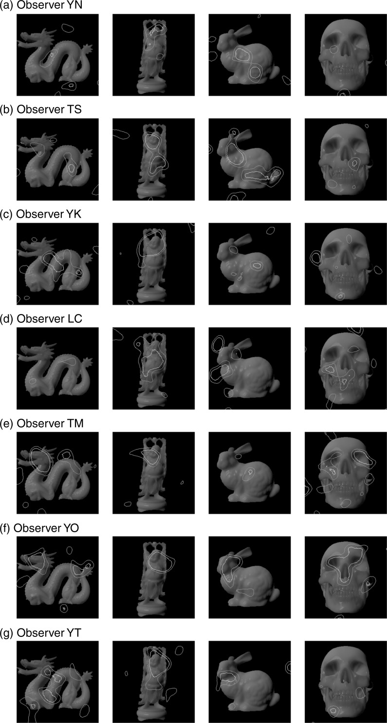
We resampled the observer's response data under the assumption (the null hypothesis) that the observer responded in a completely random way (that is, the observer did not judge perceptual translucency at all). In a resampling set, the observer's response for each trial was randomly determined. These procedures for all 3,000 trials can yield a resample-based translucency-related pattern for each object shape. We repeated this resampling procedure 10,000 times for each observer and object shape, resulting in 10,000 translucency-related patterns. Then the value of the translucency-related pattern derived from the main experiment was compared with the 10,000 resample-based translucency-related patterns. A pixel for which the value of the experimental translucency-related pattern was larger than 99% or 99.9% of the 10,000 resample-based translucency-related patterns was defined to be within the translucency-related region, which represents image regions significantly related to the perceptual translucency.

The translucency-related regions derived from the resampling procedure for all observers are shown in Figure 7. The translucency-related regions are distributed not in the entire region corresponding to the objects but in only small areas in the object image regions. This suggests that some small regions are more strongly related to the judgment of perceptual translucency than others. In addition, the positions of the translucency-related regions greatly differ between observers. For example, for Bunny, observer YN seemed to attend to the area near the center of the body, which has small luminance variations, whereas observer TS seemed to attend to the area around the neck and tail, which seems to have luminance edges. This raises the possibility that observers may use different strategies regarding where to attend in judging perceptual translucency. Namely, multiple cues for perceptual translucency might exist in the images, and observers might rely on different cues among the possible cues.

Figure 7.

Contours of translucency-related regions for all observers. The thick white line shows translucency-related regions corresponding to p < 0.001, and the thin white line shows those corresponding to p < 0.01.

To quantitatively evaluate individual differences in the translucency-related regions, we defined an index of individual differences as follows. First, we extracted “all-translucency-related regions,” which were regions included in either observer's translucency-related regions (namely, logical add of all observers' translucency-related regions). Second, for each pixel in the all-translucency-related regions, we calculated how many observers' translucency-related regions contained the pixel. Finally, we averaged these observer numbers across all pixels in all-translucency-related patterns. This averaged value was defined as the individual-difference index. This index would be 7 if the translucency-related regions of all observers were identical, while it would be 1 if the translucency-related regions of all observers were completely different. The calculated indices were 1.57 for Dragon, 2.32 for Buddha, 1.56 for Bunny, and 1.26 for Skull. These values were close to 1, suggesting the large individual differences in the translucency-related patterns, though there were some differences in the indices between the object shapes.

3.4. Image features related to perceptual translucency

Because the positions of the translucency-related regions themselves were not common across the observers as shown in Figure 7 and individual difference indices, we focused on image features common to the translucency-related regions across the observers to investigate image cues for translucency judgment.

3.4.1. Global rms contrast

Motoyoshi (2010) showed that the rms contrast of luminance of diffuse reflection components might be related to perceptual translucency, although the rms contrast did not predict strong translucency caused by the object's transmittance. We controlled the strength of the perceptual translucency via the distance parameter of subsurface scattering, only in the range in which the rms contrast should well correlate with the perceptual translucency. In this subsurface scattering range, smaller rms contrasts should induce greater perceived translucency, according to Motoyoshi (2010). Therefore, we examine the relationship between the rms contrasts of the stimulus images and the observer's responses.

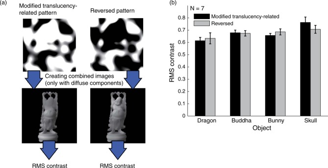
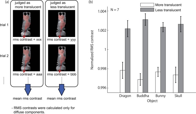
A schematic of the analysis procedure is shown in Figure 8(a). First, we calculated the rms contrasts of the stimulus images created with combined images based on the modified translucency-related patterns and with those based on the reversed modified translucency-related patterns, examples of which are shown in Figure 6(a). To calculate the rms contrast, we measured the gamma properties of the CRT monitor using Cambridge Research Systems ColorCAL2, and then we calculated the luminance of each pixel on the basis of the photometric values of images that were rendered without specular components (the specularity and glossiness parameters were set to 0%). Note that this exclusion of specular components in the luminance statistics calculation was common to all the analysis described later in this paper. The luminance rms contrasts were calculated only within the object regions. The rms contrasts for each object shape averaged across the observers are shown in Figure 8(b). The rms contrasts of the images based on modified translucency-related and reversed modified translucency-related patterns are not very different, even though the images based on the modified translucency-related pattern seem more translucent to observers, as shown in Figure 6(b). This suggests that the observers did not depend on the rms contrasts of the images when judging the perceived translucency. Analysis including the specular components also supported the same conclusion (data not shown).

Figure 8.

(a) Schematic of the analysis procedure of the global rms contrast on the basis of translucency-related patterns. (b) RMS contrast calculated from luminance of the entire image region in the images based on the modified translucency-related pattern and the reversed pattern. Specular components were excluded in this rms contrast calculation (this is common to other analyses of luminance statistics in this paper).

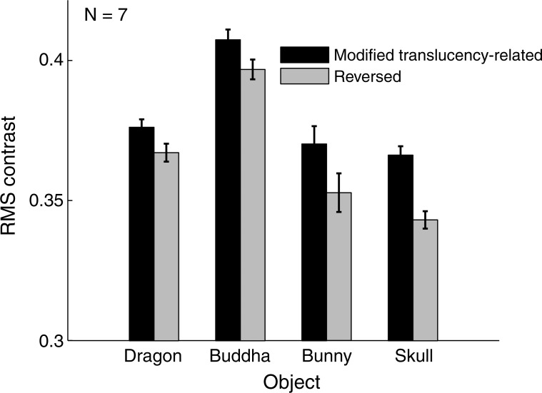
Luminance statistics (especially rms contrast) in high spatial frequency components in diffuse object images are also suggested to be important for perceptual translucency in Motoyoshi (2010). Thus, we further analyzed effects of luminance statistics of low and high spatial frequency components of an image on perceptual translucency. The analysis procedure was the same as the above analysis except that before rms contrast calculation the images were converted into low and high spatial frequency images using a digital filter whose cut-off frequency was 16 cycles/image. The results for high-spatial frequency components are shown in Figure 9 (the results for low-frequency components showed no clear tendency). The rms contrasts for images based on the translucency-related patterns were significantly higher than those based on the reversed patterns. Namely, lower rms contrast tended to yield weaker perceptual translucency. However, this relationship between rms contrast and perceptual translucency were opposite to the results of Motoyoshi; in his results, low rms contrasts in the high spatial frequency components were linked to strong perceptual translucency. The strong effects of rms contrast in the high spatial frequency images on perceptual translucency were clearly shown in his demonstration of image manipulations (his Figure 5). Thus, our correlation between the rms contrast of high-frequency components and translucency judgments may not reflect critical image features for perceptual translucency, but rather this correlation may be a byproduct produced when the observer utilized image features in local regions rather than global image features (for example, this correlation may arise if the observer relied on image regions with few edges or textures). At least in our experimental environment, local image regions might have played a more important role than global rms contrasts in high spatial frequency components.

Figure 9.

RMS contrasts in the high spatial frequency components of diffuse components in image regions based on the translucency-related pattern and its reversed patterns.

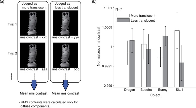
In the analysis above, the effects of the rms contrasts might have been obscured in the images created using the modified translucency-related patterns because of the simple averaging procedure to derive the translucency-related patterns, even if the rms contrast affected the observers' translucency judgment in each trial. Indeed, we confirmed that images created from different combining patterns had rms contrast differences large enough to affect perceptual translucency. Thus, as another analysis, we calculated rms contrast of a stimulus in each trial. The procedure is shown in Figure 10(a). First, we created two stimuli only with diffuse components based on the combining patterns used in each trial, though the parameter x (the signal value regarding translucency) was set to zero in order to evaluate only the effects of the combining patterns (the noise) on the observer's judgments. Then, the rms contrasts of the two images were calculated. Finally, the rms contrasts were averaged across all trials within each response class (more translucent or less translucent), for each observer and object shape. The averaged rms contrasts normalized in each object shape are shown in Figure 10(b). Again, the rms contrasts did not differ significantly between the more- and less-translucent classes, suggesting the ineffectiveness of the rms contrast based on entire object images as a cue for perceptual translucency.

Figure 10.

(a) Schematic of the analysis procedure of the global rms contrast on the basis of the observer's response and combining patterns in each trial. (b) RMS contrast in the entire image region of images the observer judged as more translucent and less translucent.

We do not think that our results disagree with those of Motoyoshi (2010). The rms contrasts he calculated from his stimuli should also, of course, be well correlated with local image statistics such as the local rms contrasts calculated only in local image regions. Therefore, the other local statistics, not the rms contrast, may be more important for judging translucency.

3.4.2. RMS contrast within translucency-related regions

As described above, the report of Motoyoshi (2010) on the effects of the rms contrast was unclear regarding whether the rms contrasts based on entire images or those based on certain local regions are important for perceptual translucency. Here, we investigate the effects of the rms contrasts calculated from local image regions, the translucency-related regions.

First, we focused on the information regarding the local rms contrast between the large- and small-scattering images. If the local rms contrasts in the translucency-related regions of the images were important for perceptual translucency, the rms contrast difference between the large- and small-scattering images should be larger in those regions than in the others. Thus, we calculated the rms contrasts in the translucency-related regions of the large- and small-scattering images with the parameter x of zero (a schematic of the procedure is shown in Figure 11(a). The obtained rms contrasts averaged across the observers are shown in Figure 11(b). The local rms contrasts of the large- and small-scattering images do not significantly differ, according to a one-tailed t-test with a significance level of 0.05. These results indicate that at least the observers did not attend to the image regions that contained larger local rms contrast cues than the other regions.

Figure 11.

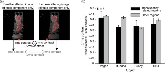
(a) Schematic of the analysis procedure for the local rms contrast difference between large- and small-scattering images. (b) Difference in rms contrast between large- and small-scattering images within translucency-related regions and other regions.

Second, we were interested in the effect of the local rms contrast on the translucency judgment in each trial. As in the third analysis of the global rms contrast, we calculated the local rms contrasts only in the translucency-related regions of the more- and less-translucent stimuli determined by the observer's responses, as shown in Figure 12(a). The local rms contrasts averaged across the trials and observers are shown in Figure 12(b). Here, significant differences appeared between the more- and less-translucent stimuli for all the object shapes according to a one-tailed t-test. In addition, t-tests for each of the observer and object shape combinations showed that the differences between the more- and less-translucent stimuli were significant in 19/28 cases. These results suggest that the observers may have relied on local rms contrasts in certain image regions, such as luminance edges created by shading patterns, when judging perceptual translucency.

Figure 12.

(a) Schematic of the analysis procedure of the local rms contrast on the basis of the observer's response and combining patterns in each trial. (b) Mean rms contrast in translucency-related regions for more translucent and less translucent images according to observers. These rms contrasts were normalized by the mean rms contrast for each object shape.

However, the effectiveness of correlating the local rms contrast with the observers' judgments of perceptual translucency may not be interesting because the translucency-related regions in the more translucent images should have tended to contain the luminance components of the large-scattering images, and thus should have contained different types of luminance features in the large-scattering images, not only the local rms contrast. In addition, the first analysis in this subsection shows no difference in the amount of information about the local rms contrast between the translucency-related regions and other regions. These results may suggest that other local statistics may be more important for perceptual translucency than the local rms contrast. We check the effects of another luminance statistic in the translucency-related regions on perceptual translucency in the following subsection.

3.4.3. Mean luminance within translucency-related regions

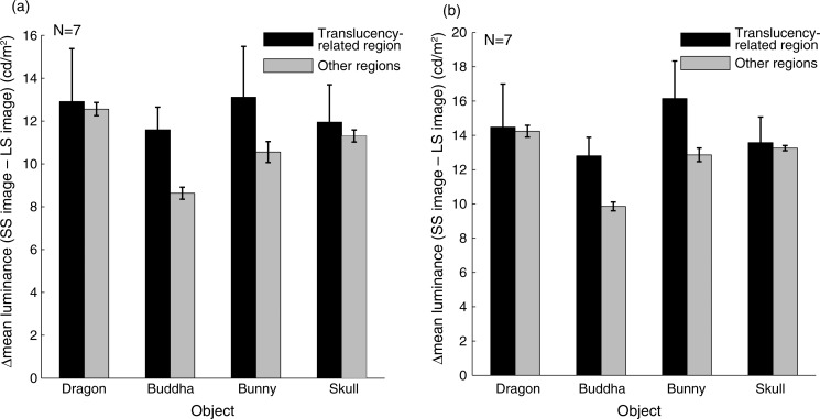
Here, we focus on the mean luminance in the translucency-related regions, a simpler image statistic than the rms contrast. If the mean luminance differences between the large- and small-scattering images were larger in the translucency-related regions than in other regions, the observer could employ the mean luminance information to perceive the translucency of the objects. In the analysis, the mean luminances of the diffuse components of the large-scattering images were differentiated from those of the small-scattering images in each of the translucency-related regions and the other regions. The mean luminance differences are shown in Figure 13(a). For all the object shapes, the luminance differences are larger in the translucency-related regions than in other regions, suggesting that the mean luminance could serve as a cue for perceptual translucency. However, as shown in Figure 2, the large-scattering images did not always contain lower luminances than the small-scattering images; in particular, the luminance relationship was reversed in image regions corresponding to the attached shadows. To deal with this luminance relationship between the large- and small-scattering images, we reanalyzed the differences in the mean absolute differences in the same way as in Figure 13(a). The results are shown in Figure 13(b). The shapes of the graphs in Figures 13(a) and (b) are quite similar. Again, the luminance differences were larger in the translucency-related regions than in other regions. Despite this tendency, the main effect of the regional difference was not statistically significant (p = 0.073, according to repeated-measures two-way ANOVA). Still, these results showed a more consistent tendency than the local rms contrast in Figure 11(b).

Figure 13.

(a) Difference in mean luminances between large- and small-scattering images within translucency-related regions and other regions. (b) Absolute difference in mean luminances between large- and small-scattering images within translucency-related regions and other regions.

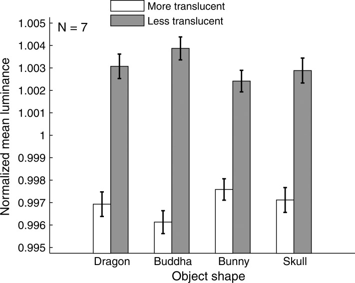
Then, we again analyzed the relationship between the mean luminance in the translucency-related region and the observer's response in each trial. The analysis procedure was quite similar to the second analysis of the local rms contrast in the previous subsection, except that the statistic to be calculated in the translucency-related regions was the mean luminance, not the rms contrast, of the diffuse components. The results are shown in Figure 14. As in Figure 12(b), the mean luminances for the more- and less-translucent images differ significantly for all the object shapes. In addition, a t-test showed that the mean luminance differences between the more- and less-translucent images in the translucency-related regions were significant for all of the observers and object shapes (28/28 cases). These results suggest that not only the local rms contrast but also the mean luminance within the translucency-related regions are well correlated with the transparency judgments of the observers. In addition, the local luminance seems to exhibit more potential as a cue for perceptual translucency than the local rms contrast, because in all the conditions the differences between the less- and more-translucent images were statistically significant, unlike the results for the local rms contrast (only 19 of 28 cases). The absolute mean luminance must not, of course, be a direct cue for judging perceptual translucency considering the luminance relationship between the large- and small-scattering images. Instead, a simplified contrast using the mean luminance in certain regions, which was calculated as a ratio of the local mean luminance and the mean luminance calculated using the entire image, can be a cue for perceptual transluc translucency.

Figure 14.

Mean luminance in translucency-related regions for more translucent and less translucent images. Values were normalized using the mean luminance for each object shape.

3.4.4. Prediction of observers' responses based on luminance statistics

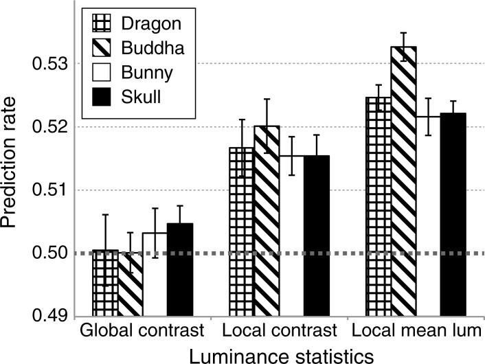
In the analysis above, we investigated how well the luminance statistics were correlated with the perceptual translucency. In addition, it should also be valuable to estimate the observers' responses from these luminance statistics to check how those features affected judgments of relative translucency. Thus, we calculated the ratio of the number of trials for which predictions based on the luminance statistics were the same as the observers' actual responses to the number of all trials. In this analysis, the predictions were made for an image pair in each trial on the basis of only the relative amount of each of the luminance statistics: global rms contrast, local (within translucency-related regions) rms contrast, and local (within translucency-related regions) mean luminance. An image with smaller global rms contrast, smaller local rms contrast, or smaller mean luminances was classified as a more translucent image (these estimation directions based on the luminance statistics were determined according to our analysis results shown in Figures 10, 12, and 14). The concordance rates between the observers' responses and the estimations for each object shape and luminance statistics are shown in Figure 15. First, the concordance rates are clearly quite low; they were all less than 0.54 (the chance level was 0.5). These results show that the effectiveness of these image luminance statistics as cues for perceptual translucency was quite low. However, differences in the concordance rates seem to exist between the luminance statistics; the rates for the global rms contrast lay around the chance level, indicating the ineffectiveness of the global rms contrast in predicting the observers' responses. In contrast, the rates for local rms contrast and local mean luminance were significantly higher than the chance level, suggesting the effectiveness of these luminance statistics in estimating observers' translucency responses. In addition, the rates for the local mean luminance were higher than those for the local rms contrast. Because these two luminance statistics were derived from the same local regions, these results again suggest that the mean luminance in translucency-related regions can be a more plausible candidate as a cue for perceptual translucency than the local rms contrast.

Figure 15.

Rates of concordance between the observers' responses in the experiment and the response estimations made using three luminance statistics for each object shape.

3.4.5. Shading pattern within translucency-related regions

We do not know why the observers individually attended to certain spatial regions when judging perceptual translucency, even though local image features such as mean luminance or local rms contrast may be partially correlated with observers' responses. For example, if the local mean luminance is an important cue for perceptual translucency, why does the observer use luminance information in specific spatial regions and how does the observer know that the specific regions are important to estimate translucency?

One such candidate is the luminance difference between the large- and small-scattering images. If observers could identify the image regions where the luminances differ greatly between the large- and small-scattering images, they may attend to such regions in judging the object's translucency. In our stimuli, the luminance differences between the large- and small-scattering images are physically different on two types of surfaces, those that face the light source (illuminated surfaces) and those facing away from the light source (attached shadow surfaces). This is the result of our illumination setting (a point light source in front of the object) and our method of controlling the perceptual translucency. For the large-scattering images, the luminances of the illuminated surfaces were lower and those of the shaded surfaces were higher than in the small-scattering images owing to the effects of subsurface scattering of incident light. This tendency can be observed in the two images on the left in Figure 2, though the absolute luminance differences seem much larger for the illuminated surfaces than for the shaded surfaces.

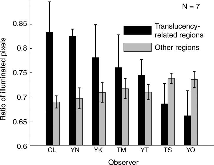
Here, we suggest two hypotheses; one hypothesis is that the observer attends to spatial regions where the luminance differences between the large- and small-scattering images are large specifically for our stimuli (that is, the illuminated surfaces), and the other is that the observer attends to spatial regions where luminance differences generally occur between the large- and small-scattering images (that is, both the illuminated and shaded surfaces). To investigate this issue, we calculated the ratio of the pixel numbers of illuminated surfaces to those of shaded surfaces in the translucency-related regions. The illuminated surface pixels were defined as pixels whose luminances were lower in the large-scattering images than in the small-scattering images, and the shaded surfaces were defined as pixels whose luminances were higher in the large-scattering images than in the small-scattering images.

The calculated pixel ratios for each observer are shown in Figure 16. This figure shows that individual observers differed greatly in which image regions they attended to. Five of the seven observers seem to have given more importance to the illuminated surfaces than to the shaded surfaces, as expected from the larger luminance differences between images with different subsurface scattering parameters. However, interestingly, the other two observers tended to attend to the shaded surfaces more than to the illuminated surfaces, although this tendency was not statistically significant. These observers might have relied on the general rule that the luminances of the shaded surfaces, which are higher in the large-scattering images, could also be a cue for perceptual translucency; that is, the observers do not always obey the hypothesis above and attend only to image regions whose luminance differences between the large- and small-scattering images were large.

Figure 16.

Ratio of the pixel numbers of surfaces directly illuminated by the light source to those corresponding to the attached shadow in translucency-related regions and other regions. Values are averages across the four object shapes.

4. General discussion

We aimed to extract local spatial regions within CG images that can be important for perceptual translucency using a psychophysical reverse-correlation approach. The stimulus contained two CG images, which were combinations of large- and small-scattering images according to a random spatial profile (the combining pattern). The observer judged which of the two images seemed to be more translucent. We analyzed the relationship between the combining patterns and the observer's responses. The results showed that some spatial regions were more related to perceptual translucency judgments than others, although the positions of these regions varied between the observers. Then, we analyzed the image features related to the extracted regions and found that (1) the rms contrasts of luminances within entire images or within the extracted regions may not be an important cue for perceptual translucency, (2) the mean luminances in the extracted regions may be important in part for perceptual translucency, possibly via a simplified luminance contrast calculated as the ratio between the mean luminance based on entire images and that based on the extracted image regions, and (3) each observer judged perceptual translucency by placing more importance on either the illuminated surfaces or the shaded surfaces, depending on the observer, not only on the regions where the luminance differences between the large- and small-scattering images were large.

Motoyoshi (2010) argued the relationship between perceptual translucency and image features based on entire images. He suggested that the spatial relationship between specular highlights and the shading luminance patterns or rms contrast of the shading patterns can be cues for the perceptual translucency within a limited range, which can be controlled only by the depth parameter of subsurface scattering. In this article, we focused on the effects of rms contrast. However, we did not find that the rms contrast calculated from the entire stimulus image made any contribution to the perceptual translucency. This suggests that the rms contrast calculated from entire object images is not very important to perceptual translucency. We guess that the relationship between rms contrast and perceptual translucency demonstrated by Motoyoshi (2010) may arise from other image features correlated with both perceptual translucency and the global rms contrast. In any case, the global rms contrast should not be a direct cue for perceptual translucency.

Certain image regions should contribute more strongly to perceptual translucency than others, as demonstrated in our results by the fact that only some local regions, which differed between observers, were extracted as important regions for perceptual translucency (the translucency-related regions). In our stimuli, in which all the luminance components were controlled by the combining patterns, different types of image features based on the luminances in the translucency-related regions may be correlated with the observers' responses. However, a simpler luminance statistic, the mean luminance, may be more plausible as a cue for perceptual translucency than the rms contrast, to the extent investigated in this study. To check the influence of local luminance on perceptual translucency, we changed luminances of the diffuse components in the small-scattering images based on the translucency-related patterns. In this manipulation, a luminance value in each pixel was multiplied with the value of each pixel in the translucency-related patterns (or reversed-translucency-related patterns) whose values were normalized into the range from 0.85 to 1.0. Example images created with such luminance manipulations are shown in Figure 17. The results showed that the luminance manipulations only slightly affect perceptual translucency by itself, if any. These results suggest that the local luminance should not be a critical cue but can have only small effects on perceptual translucency by itself. The observer may rely on, for example, the ratio of the mean luminances in certain image regions to those in entire image regions, or relationship between local luminance other image features like local contrast. Fleming and Bulthoff (2005) suggested the importance of local regions (especially regions corresponding to thin portions of objects) and of the luminance histogram for translucency perception. Their suggestions are corresponding to our results in that the certain image regions are more important to predict perceptual translucency than the other regions, although local cues for translucency perception contained in such regions should be more carefully investigated in future research. In addition, Fleming and Bulthoff suggested the importance of the light bleeding through the shadowed region of an object on perceptual translucency. Our analysis of the translucency-related regions in regard to the pixel numbers in the illuminated and shadowed regions also suggested that some observers utilized image information within the shadowed regions despite the larger luminance difference between the large- and small-scattering images in the illuminated regions than in the shadowed regions. These results suggest the importance of luminance information in the shadowed regions, as in Fleming and Bulthoff.

Figure 17.

Effects of luminance adjustment on small-scattering images. These results are created based on the translucency-related patterns (and its reversed patterns) of the observer LC.

Our simple illumination environment, which contained only a point light source, differed greatly from typical illumination environments. The realism of CG images is known to increase dramatically when they are rendered under natural illumination environments (Debevec, 1998; Hwang, 2004). In addition, the perceived surface qualities of objects, such as glossiness, depend strongly on the illumination environment (Doerschner, Boyaci, & Maloney, 2010; Fleming, Dror, & Adelson, 2003; Olkkonen & Brainard, 2011). Therefore, the relationship between perceptual translucency and image statistics found in our results may be observed only in our illumination environment. For example, the mean luminance based on an entire image of ours decreased with increasing translucency by increasing the distance parameter of subsurface scattering. This should be specific to our illumination environment, where the back of the object was completely black, and the effects of the blackness emerged even from the front surface of the object owing to the effects of subsurface scattering. Instead, the mean luminance difference between the distance parameters should become much smaller if we employ natural illumination maps such as those used in different studies regarding material perception (e.g., Fleming et al., 2003; Motoyoshi, 2010). Thus, we do not think that the mean luminance of the image acts as a cue for perceptual translucency. However, a type of simplified contrast, such as the luminance ratio between an entire image region and certain local image regions, may still contribute to perceptual translucency, as shown in our results. This strategy seems valid even for CG images rendered under a natural illumination map if we look into the relationship between the luminance patterns of translucent and opaque images (Figure 3 of Motoyoshi, 2010, second row). We speculate that the contrast relationship between the mean luminances only in several image regions is important as a cue for perceived translucency, although it remains unclear why the observers relied on specific image regions. In addition, although previous studies suggested the importance of specular highlights for perceptual translucency (Fleming & Bulthoff, 2005; Motoyoshi, 2010), we did not find any relationship between the positions of specular highlights and translucency-related regions (data not shown). General image features in local regions that can be important for perceptual translucency have to be clarified in future research. Reverse-correlation methods, such as the one we employed, may be helpful for extracting local image regions containing image cues for perceptually judging surface qualities.

In our results, large individual differences were observed, especially in the spatial positions of the translucency-related regions. We believe that these individual differences did not emerge from just the noise in our reverse-correlation procedures that were not relevant to perceptual translucency, because the combined images based on the modified translucency-related patterns induced perception of more translucent objects (Figure 6b), suggesting that some spatial regions shown in modified translucency-related patterns can more strongly affect the perceptual translucency than the other regions. This individual variability raises the possibility that there were many candidate image regions containing cues for judging translucency whose strengths of effects on perceptual translucency may not be very different. Because in our reverse-correlation procedure only the relative, not absolute, amounts of the effects can be extracted from the observers' responses, the results can be easily unstable if there were many spatial regions magnitudes of whose effects on perceptual translucency were not very different. In addition, some artifacts in our stimuli that were not directly related to perceptual translucency may have affected observers' translucency judgments. For example, the translucency-related regions in Buddha were located around the face of the Buddha for almost all the observers. From these results, we cannot exclude the possibility that they were obtained just because the observers' attentions were attracted to human faces (e.g., Hershler & Hochstein, 2005; but see VanRullen, 2006) irrespective of the efficiency of luminance cues for translucency judgments in these regions. This face effect, if it exists, must be an artifact in our analysis. Similar artifacts, which may affect the spatial positions of the observers' attention, may contaminate our results regarding the spatial image regions important for perceptual translucency. This type of attentional artifact may be difficult to remove completely from the results of psychophysical reverse-correlation methods. In future works, the effects of some possible factors contributing to perceptual translucency extracted from a reverse-correlation method must be checked in conventional parametric experiments in which the factors are defined as experimental variables.

The inhomogeneous perception of surface qualities on our stimuli may have possibly affected our results. We combined luminance components of a large- and a small-scattering image based on spatial random pattern. This corresponds to the blend of a large- and a small-scattering image depending on image regions, which may have caused perception of inhomogeneous surface qualities. Indeed, some of our observers reported that they occasionally felt that the translucency of the images was not uniform across spatial regions. The psychophysical reverse-correlation method for surface quality perception employing spatial random patterns may not completely avoid the effects of this inhomogeneous perception of surface qualities in principle. However, our observers also reported that our task, comparison of translucency between two images based on whole image regions, was viable regardless of the inhomogeneous perception, suggesting that strangeness feeling of inhomogeneous perception did not largely affect the translucency judgments, if any, though such inhomogeneous perception may have acted as a noise in our results.

In conclusion, we extracted spatial regions in CG images that were related to observers' judgments of translucency and analyzed some image features included in these regions. Some spatial regions may be more effective for translucency judgments than others, although there were large individual differences in the positions of the regions. The rms contrast of the shading patterns calculated in the entire image region did not explain the observers' performance. Instead, some local image statistics performed somewhat better; the local mean luminance of the shading patterns in the extracted regions can be a more plausible, simpler cue for translucency judgments than the rms contrasts within the extracted regions, though mean luminance does not directly induce perceptual translucency by itself (possibly its effects depend on the ratio to the mean luminance calculated from entire images, or collaboration with other luminance statistics). In addition, individual observers seemed to attend to either the illuminated surfaces or the shaded surfaces, which exhibit luminance differences depending on different translucencies in opposite directions. Future research should examine how observers can find effective spatial regions when making translucency judgments.

References

- Ahumada A. J., Jr. Perceptual classification images from Vernier acuity masked by noise. Perception. 1996;25 doi: 10.1068/v96l0501. ECVP Abstract Supplement. [DOI] [Google Scholar]
- Anderson B. L., Kim J. Image statistics do not explain the perception of gloss and lightness. Journal of Vision. 2009;9(11):10. doi: 10.1167/9.11.10. (1–17) [DOI] [PubMed] [Google Scholar]
- Boivin S., Gagalowicz A. Image-based rendering of diffuse, specular and glossy surfaces from a single image. Proceedings of the 28th Annual Conference on Computer Graphics and Interactive Techniques, Los Angeles, CA, USA. 2001. pp. 107–116. [DOI]
- Brainard D. H. The psychophysics toolbox. Spatial Vision. 1997;10(4):433–436. doi: 10.1163/156856897x00357. [DOI] [PubMed] [Google Scholar]
- Debevec P. E. Rendering synthetic objects into real scenes: Bridging traditional and image-based graphics with global illumination and high dynamic range photography. Proceedings of SIGGRAPH. 1998;98:189–198. doi: 10.1145/280814.280864. [DOI] [Google Scholar]
- Doerschner K., Boyaci H., Maloney L. T. Estimating the glossiness transfer function induced by illumination change and testing its transitivity. Journal of Vision. 2010;10(4):8. doi: 10.1167/10.4.8. (1–9) [DOI] [PMC free article] [PubMed] [Google Scholar]
- Fleming R. W., Bulthoff H. H. Low-level image cues in the perception of translucent materials. ACM Transactions on Applied Perception. 2005;2(3):346–382. doi: 10.1145/1077399.1077409. [DOI] [Google Scholar]
- Fleming R. W., Dror R. O., Adelson E. H. Real-world illumination and the perception of surface reflectance properties. Journal of Vision. 2003;3(5):347–368. doi: 10.1167/l3.5.3. [DOI] [PubMed] [Google Scholar]
- Foster D. H. Color constancy. Vision Research. 2011;51(7):674–700. doi: 10.1016/j.visres.2010.09.006. [DOI] [PubMed] [Google Scholar]
- Gold J. M., Murray R. F., Bennett P. J., Sekuler A. B. Deriving behavioural receptive fields for visually completed contours. Current Biology. 2000;10(11):663–666. doi: 10.1016/S0960-9822(00)00523-6. [DOI] [PubMed] [Google Scholar]
- Hershler O., Hochstein S. At first sight: A high-level pop out effect for faces. Vision Research. 2005;45(13):1707–1724. doi: 10.1016/j.visres.2005.07.009. [DOI] [PubMed] [Google Scholar]
- Hwang G. T. Hollywood's master of light. Technology Review. 2004;107:70–73. [Google Scholar]
- Jensen H. W., Buhler J. A rapid hierarchical rendering technique for translucent materials. ACM Transactions on Graphics. 2002;21(3):576–581. doi: 10.1145/566654.566619. [DOI] [Google Scholar]
- Kim J., Marlow P., Anderson B. L. The perception of gloss depends on highlight congruence with surface shading. Journal of Vision. 2011;11(9):4. doi: 10.1167/11.9.16. (1–19) [DOI] [PubMed] [Google Scholar]
- Mangini M. C., Biederman I. Making the ineffable explicit: Estimating the information employed for face classifications. Cognitive Science. 2004;28(2):209–226. doi: 10.1016/j.cogsci.2003.11.004. [DOI] [Google Scholar]
- Marlow P. J., Kim J., Anderson B. L. The perception and misperception of specular surface reflectance. Current Biology. 2012;22(20):1–5. doi: 10.1016/j.cub.2012.08.009. [DOI] [PubMed] [Google Scholar]
- Metelli F. The perception of transparency. Scientific American. 1974;230(4):90–98. doi: 10.1038/scientificamerican0474-90. [DOI] [PubMed] [Google Scholar]
- Motoyoshi I. Highlight-shading relationship as a cue for the perception of translucent and transparent materials. Journal of Vision. 2010;10(9):6. doi: 10.1167/10.9.6. (1–11) [DOI] [PubMed] [Google Scholar]
- Motoyoshi I., Nishida S., Sharan L., Adelson E. H. Image statistics and the perception of surface qualities. Nature. 2007;447(7141):206–209. doi: 10.1038/nature05724. [DOI] [PubMed] [Google Scholar]
- Murray R. F. Classification images: A review. Journal of Vision. 2011;11(5):2. doi: 10.1167/11.5.2. (1–25) [DOI] [PubMed] [Google Scholar]
- Nestor A., Tarr M. J. Gender recognition of human faces using color. Psychological Science. 2008;19(12):1242–1246. doi: 10.1111/j.1467-9280.2008.02232.x. [DOI] [PubMed] [Google Scholar]
- Olkkonen M., Brainard D. H. Joint effects of illumination geometry and object shape in the perception of surface reflectance. i-Perception. 2011;2:1014–1034. doi: 10.1068/i0480. [DOI] [PMC free article] [PubMed] [Google Scholar]
- Ramamoorthi R., Hanrahan P. A signal-processing framework for inverse rendering. Proceedings of the 28th Annual Conference on Computer Graphics and Interactive Techniques, Los Angeles, CA, USA. 2001. pp. 117–128. [DOI]
- Sharan L., Li Y. Z., Motoyoshi I., Nishida S., Adelson E. H. Image statistics for surface reflectance perception. Journal of the Optical Society of America, A. 2008;25(4):846–865. doi: 10.1364/JOSAA.25.000846. [DOI] [PubMed] [Google Scholar]
- Singh M., Anderson B. L. Toward a perceptual theory of transparency. Psychological Review. 2002;109(3):492–519. doi: 10.1037//0033-295x.109.3.492. [DOI] [PubMed] [Google Scholar]
- VanRullen R. On second glance: Still no high-level pop-out effect for faces. Vision Research. 2006;46(18):3017–3027. doi: 10.1016/j.visres.2005.07.009. [DOI] [PubMed] [Google Scholar]