A spatial time-to-event approach for estimating associations between air pollution and preterm birth

Summary

The paper describes a Bayesian spatial discrete time survival model to estimate the effect of air pollution on the risk of preterm birth. The standard approach treats prematurity as a binary outcome and cannot effectively examine time varying exposures during pregnancy. Time varying exposures can arise either in short-term lagged exposures due to seasonality in air pollution or long-term cumulative exposures due to changes in length of exposure. Our model addresses this challenge by viewing gestational age as time-to-event data where each pregnancy becomes at risk at a prespecified time (e.g. the 28th week). The pregnancy is then followed until either a birth occurs before the 37th week (preterm), or it reaches the 37th week, and a full-term birth is expected. The model also includes a flexible spatially varying baseline hazard function to control for unmeasured spatial confounders and to borrow information across areal units. The approach proposed is applied to geocoded birth records in Mecklenburg County, North Carolina, for the period 2001–2005.We examine the risk of preterm birth that is associated with total cumulative and 4-week lagged exposure to ambient fine particulate matter.

1. Introduction

Preterm birth, which is defined as gestational age at delivery of less than 37 weeks, is linked to significant neonatal morbidity and mortality (Lorenz et al., 1998; Goldenberg et al., 2008; Saigal and Doyle, 2008), long-term health and developmental problems (Swamy et al., 2008; Moster et al., 2008) and medical costs (Institute of Medicine, 2006). There is a growing interest in examining the association between environmental exposures during pregnancy and adverse birth outcomes. Population studies have found consistent positive associations between ambient air pollution levels and low birth weight; however, epidemiological evidence remains mixed for preterm birth (S̆rám et al., 2005; Bosetti et al., 2010).

Studies of air pollution and preterm birth utilize large birth record databases that provide extensive information on individual live births. For each birth, average exposures to air pollutants over specific susceptible pregnancy windows are then derived from air quality measurements. The most common analytic approach is carried out via logistic regression where preterm versus full-term births are treated as binary outcomes (Wilhelm and Ritz, 2005; Huynh et al., 2006; Leem et al., 2006; Ritz et al., 2007; Brauer et al., 2008). This approach is most suitable to examine exposure metrics that do not vary during pregnancy, such as the first 6 weeks since conception, or the first and second trimester (Woodruff et al., 2009). However, many long-term and short-term exposure windows are time varying because ambient pollution levels exhibit strong seasonality.

Consider using the average air pollution level over the entire pregnancy to estimate the long-term effect of air pollution on preterm birth. In a logistic regression model, bias in risk estimates may arise with this overall exposure metric because the lengths of exposure differ between preterm and full-term births. For pregnancies that are conceived in the winter months, preterm births are more likely to experience lower average exposure than full-term births. This is because full-term births have a longer exposure window extending into the summer months when ambient pollution concentrations are typically higher. However, for pregnancies that are conceived in the summer, preterm births experience higher exposure levels compared with full-term births. The direction and magnitude of the bias therefore depend on the seasonality in both air pollution and the number of on-going pregnancies in the population (Darrow et al., 2009b). This challenge is also present in estimating the effect of air pollution during the third trimester (27th week till birth).

Estimating the short-term effects of air pollution on preterm birth during late pregnancy is also problematic by using logistic regression. A common approach is to capture late pregnancy exposure with a window before delivery (e.g. 4 weeks or 6 weeks before birth). However, this exposure metric does not coincide with the period when a full-term birth is at risk of being preterm. For example, consider a 40-week full-term pregnancy that experienced high exposure during the month before birth. This pregnancy will contribute to a protective effect of air pollution even though it cannot be preterm after week 37. Using only the weeks before birth also discards data from earlier weeks that are informative about the short-term effect.

The main contribution of this paper is to describe a model for preterm birth that addresses the above challenges in estimating the effects of long-term and short-term exposures that are time varying during pregnancy. This is accomplished by viewing gestational age as time-to-event (survival) data where each pregnancy enters the risk set at a prespecified time (e.g. the 28th week). The pregnancy is then followed until either a birth occurs before the 37th week (preterm), or it reaches the 37th week and a full-term birth is expected. Therefore, we align the data such that pregnancies are compared with each other only during a window at risk of being preterm (i.e. 28th–37th week). This allows us to examine

1. long-term effects by using a time varying cumulative average instead of an average over the entire pregnancy and

2. short-term effects by using a time varying lagged average instead of a fixed period defined before delivery.

The risk estimates from the time-to-event approach have similar interpretations to that obtained from a time series analysis stratified by gestational week (Darrow et al., 2009a). In a time series analysis, the outcome of interest is the daily number of preterm births aggregated over a geographic region. The corresponding daily exposure metric is obtained by averaging air pollution exposures across all on-going pregnancies on each day. The time series design also overcomes the challenges in defining time varying exposures because the aggregate exposure is allowed to vary between days. The time series design was originally motivated by the issue of unmeasured confounders. In contrast, our proposed approach utilizes the full spatial and temporal contrast in air pollution levels and can control for individual level covariates. Moreover, a time series analysis has limited power to detect long-term effects because considerable temporal variation in the exposure is removed when controlling for seasonality in preterm births.

In studies that rely on birth certificate data, the issue of residual confounding due to unmeasured risk factors is well recognized because the health outcome is compared across space and time (Northam and Knapp, 2009; Strickland et al., 2009). Examples of known risk factors for preterm birth that are typically not available from birth certificates include the mother’s socio-economic status, maternal body mass index, level of stress and anxiety, amount of physical work, the quality of the built environment and infections status. Often these factors may also, at least partially, determine the amount of personal exposure to air pollution due to outdoor sources. We control for unmeasured spatial confounders by including a flexible baseline hazard model that is spatially varying. This approach also allows us to borrow information across spatial units to estimate the baseline hazards at locations with small numbers of births.

Spatially referenced survival models often account for association between nearby regions by including a random effect (frailty) for the region of residence in the linear predictor, and smoothing the frailties by using a Gaussian spatial model (Banerjee et al., 2003). Although this approach allows different regions to have different baseline risks, it assumes that the general shape of the survival curve is the same for each region after accounting for the spatial frailty term. For example, this does not allow for some regions to have elevated risk very early in pregnancy but low risk late in the pregnancy. For continuous survival data, one generalization of the frailty model is to use an accelerated failure time model, i.e. suitably transform the survival times and model the transformed responses by using linear regression while allowing the mean and the entire shape of the residual distribution to vary spatially. Many models for the spatially varying residual density exist; see for example Griffin and Steel (2006), or Reich and Fuentes (2007). In contrast, with the model for continuous survival data that was described above, the North Carolina birth certificate records gestational age as the number of completed weeks. Therefore, we propose a simpler model for discrete time survival data.

We apply the proposed model to estimate the total cumulative and 4-week lag effects of ambient particulate matter that is less than 2.5 μm in diameter (PM_2.5). We treat ambient PM_2.5-concentration as a surrogate measure for personal exposure to fine particulate matter from outdoor sources. The PM_2.5-mass represents a chemically diverse mixture of solids and liquids that arise from combustion processes. Exposure to PM_2.5-pollution has been associated with numerous health outcomes including mortality, emergency department visits and hospital admissions (Pope and Dockery, 2006). The biological mechanisms by which particulate matter might affect preterm birth focus on initiation of the inflammation pathway (Kannan et al., 2006).

The remainder of this paper is organized as follows. Section 2 gives the general modelling framework of our discrete time spatial survival model for preterm birth. Section 3 describes the air pollution data and a data set of geocoded births from Mecklenburg County, North Carolina, for the period 2001–2005. Because past studies predominantly use logistic regression to analyse preterm birth, Section 4 describes a simulation study that compares the model proposed and the standard approach that treats prematurity as a binary outcome. We highlight the potential bias in risk estimates when surrogate time invariant exposures (e.g. pregnancy average or 4 weeks before birth) are used instead of time varying exposures (e.g. cumulative average or 4-week lag). Results from the health analysis are given in Section 5. Finally, discussion and future work appear in Section 6.

2. Spatial time-to-event model for preterm birth

For pregnancy i, we observe the follow-up time t_i, an indicator of whether the pregnancy was censored c_i, the spatial location s_i and a vector of p potentially time-dependent covariates X_i(t) = (X_1i(t), … , X_pi(t))’. We assume a discrete domain for spatial locations. For example, in our application s_i represents census tracts in Mecklenburg County. We also assume a discrete domain for event times because gestational age is typically recorded as the number of completed weeks. We define gestational weeks 28–36 as the at-risk period for a pregnancy being preterm. For preterm births with gestational age less than 37 weeks, t_i represents the completed week of gestation and c_i = 0. Full-term births of at least 37 weeks are censored at week 36 (t_i = 36 and c_i = 1) because they are no longer at risk of being preterm. Therefore, under this modelling framework (which is illustrated in Fig. 1),

1. no censoring occurs between gestational weeks 28–35,

2. all preterm births experienced an event and

3. all full-term births are censored.

Fig. 1.

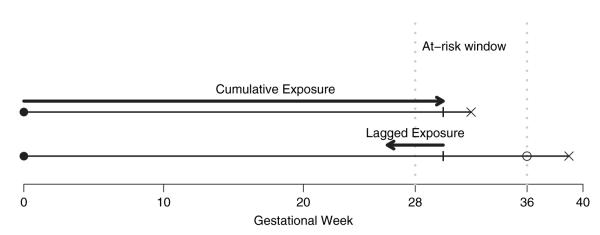
A time-to-event approach for preterm birth and air pollution: a preterm birth and a full-term birth are shown with pregnancywide cumulative exposure and 4-week lagged exposure given at week 30 (●, conception date; x, birth date; 엯, censored)

The model is defined through the event hazard rate, π{X_i(t), s_i, t}∈[0, 1], which is the probability of birth for pregnancy i at week t given that pregnancy i reaches t. This implies the survival probability

$$P(t_i>m)=\prod _{t=1}^m[1-\pi \{{\mathbf{X}}_i\left(t\right),s_i,t\left\}\right],$$ (1)

i.e. the usual life table model. We model the discrete event hazard rate by using spatial probit regression:

$$\pi \left\{\mathbf{X}\right(t),s_i=s,t\}=\Phi \left\{{\beta }_0\right(s,t)+{\mathbf{X}}_i{\left(t\right)}^{\prime }\beta \},$$ (2)

where Φ is the standard normal distribution function and β is the vector of regression coefficients. The probit link is chosen to facilitate Bayesian inference by using Markov chain Monte Carlo sampling and other link functions may be considered, e.g. a logistic link (Holmes and Held, 2006). Parameter β₀(s, t) determines the baseline risks (the event rate for a subject with X_1i(t) = … = X_pi(t)=0). Because β₀(s, t) varies with both space and time, this model spans the entire class of baseline models on this discrete domain of s_i ∈ {1, … , S} and t ∈ {28, … , 36}, where S is the total number of discrete spatial units in the study region.

Let β₀(s, t) = η + μ(s) + γ(t) + θ(s,t), where η is the overall average, μ(s) is a spatial effect, γ(t) is a temporal effect and θ(s, t) is the space–time interaction. Since the spatial terms μ = (μ(1), … , μ(S))’ are discrete areal units, we model them by using the conditionally auto-regressive (CAR) model (Besag, 1974). This spatial model is specified through spatial adjacencies. Let s~s’ indicate that regions s and s’ are spatial neighbours and m_s be the number of spatial neighbours of region s. The CAR model is often defined through the full conditional distribution of μ(s) given μ at all other locations. The full conditional distribution is Gaussian with

$$E\left\{\mu \right(s)\mid \mu (s^{\prime }),s^{\prime }\ne s\}={\rho }_{\mu }\sum _{s^{\prime }\sim s}\mu \left(s^{\prime }\right)∕m_s,$$ (3)

$$V\left\{\mu \right(s)\mid \mu (s^{\prime }),s^{\prime }\ne s\}={\sigma }_{\mu }^2∕m_s.$$ (4)

The full conditional mean is proportional to the average of the spatial neighbours, where ρ_μ ∈ [0, 1] controls the degree of spatial association, and the variance is controlled by ${\sigma }_{\mu }^2>0$. The joint model for the vector μ is multivariate normal with mean 0 and covariance ${\sigma }_{\mu }^2{(M_s-{\rho }_{\mu }{C}_s)}^{-1}$, where the (s, s’) element of C_S is C_S(s, s’) = I(s~s’) and M_S is diagonal with diagonal elements ∑_s’≠s C_S(s,s’)=m_s. We denote this model as $\mu \sim \text{CAR}({\rho }_{\mu },{\sigma }_{\mu }^2,C_s)$.

The temporal effects γ = (γ(28), … , γ(36))’ control the temporal average baseline hazard function. The vector γ has a lag 1 auto-regressive model which can be written $\gamma \sim \text{CAR}({\rho }_{\gamma },{\sigma }_{\gamma }^2,C_T)$, where C_T is the 9 × 9 temporal adjacency matrix with (t, t’) element equal to I(∣t – t’∣ = 1). The spatiotemporal random effects have the dynamic spatial model (Banerjee et al., 2003)

$$\theta (s,t)={\rho }_{\theta }\theta (s,t-1)+\delta (s,t),t=29,\dots ,36,$$ (5)

where ρ_θ ∈ (0, 1) and ${\delta }_t={\left(\delta \right(1,t),\dots ,\delta (S,t\left)\right)}^{\prime }\sim \text{CAR}({\rho }_{\delta },{\sigma }_{\delta }^2,C_s)$. For identification purposes, we fix θ(s, 28) = 0 for all s.

The above baseline hazard function model has several special cases. If θ(s, t) ≡ 0, then β₀(s, t) η + μ(s) + γ(t), and the baseline risk function varies spatially only through the spatial frailties μ(s). Therefore the shape of the risk function for all regions is constant and controlled by γ. If ρ_μ = ρ_δ = 0, then the baseline risk functions are exchangeable across locations, and hierarchically centred on η + γ.

Inference is carried out in a Bayesian framework by specifying priors for the model parameters. Parameter η and each component of β are assigned N(0, 100²). The variances ${\sigma }_{\mu }^2$, ${\sigma }_{\gamma }^2$ and ${\theta }_{\theta }^2\sim$ gamma(a₁, b₁). Following Kelsall et al. (1999), we take a₁ = 0:5 and b₁ = 0:005. The CAR association parameters ρ_μ, ρ_γ, ρ_θ, ρ_δ ~ beta(a₂, b₂). We discretize the prior to 1000 equally spaced points spanning [0,1] and, to give an uninformative prior, we take a₂ = b₂ = 1.

For each pregnancy, we augment the data (c_i, t_i) to (Y_i(28), … , Y_i(t_i)), where Y_i(t) = 0 for t < t_i and Y_i(t_i) = 1 – c_i. Therefore, at each time point during the pregnancy, Y_i(t) indicates whether a preterm birth occurred. The model for pregnancy i can then be written as Y_i(t)~Bernoulli[Φ{β₀(s, t)+X_i(t)’β}], independent across time. The Bernoulli model for Y_i(t) is equivalent to the model Y_i(t) = I{Z_i(t) > 0}, where Z_i(t) is a latent variable with Z_i(t) ~ N {β₀(s,t) + X_i(t)’ β, 1}.

After introducing the latent variables Z_i(t), the model is entirely conjugate, and we used Gibbs sampling (Casella and George, 1992) to analyse the posterior distributions of all unknown parameters. All analysis was carried out in R 2.8.0 (R Development Core Team, 2009). We generated 20 000 samples and discarded the first 5000 samples as burn-in. Convergence was monitored by using trace plots and auto-correlation plots for several representative parameters. In the on-line supplementary material, we describe the Markov chain Monte Carlo algorithm in detail and provide the R code for fitting the spatial survival model.

3. Health and exposure data

Birth data for Mecklenburg County were obtained from the North Carolina detailed birth record database. Mecklenburg County is the most populous county in North Carolina and contains the city Charlotte. We included all pregnancies that were conceived from the period 2001–2005 using the clinical estimate of gestation in the birth record to back-calculate the date of conception. We restricted the analysis to singleton live births with birth weight 400 g or more and no congenital anomalies. We further restricted the data set to those mothers aged 15–44 years who self-declared as non-Hispanic white, non-Hispanic black or Hispanic.

Daily PM_2.5-data were obtained from the statistically fused air quality database (http://www.epa.gov/esd/land-sci/lcb/lcb_sfads.html). The database is a recent product from the US Environmental Protection Agency that provides predicted daily PM_2.5-concentration averaged over contiguous 12 km × 12 km grid cells. We chose this data set because monitors in the air quality system network typically measure PM_2.5 only every third or sixth day. The database predictions are based on a Bayesian space–time hierarchical model (McMillan et al., 2009) that combines

1. PM_2.5-data from the air quality system network and

2. outputs from the models-3–community multiscale air quality model (Byun and Schere, 2006), which is an air quality model that simulates the complex interactions between weather and air pollutants on the basis of atmospheric chemistry and physics. Although this model provides higher spatial and temporal resolution compared with the air quality system network, its output is known to exhibit bias, particularly for capturing short-term variation between days (Mebust et al., 2003). The statistically fused air quality database attempts to adjust the bias in the community multiscale air quality model by using the observed PM_2.5-concentrations from the air quality system network.

Maternal residential addresses at the time of delivery were geocoded to the street block level by using ArcGIS 9.3 software (Esri, Redlands, California). We used 2006 topologically integrated geographic encoding and referencing street data from the US Census Bureau as the spatial reference file. The geocoding success rate was 97.1%, owing to invalid, missing or unmatched addresses. Using the latitude and longitude co-ordinates that were delivered by the geocoding process, we linked each pregnancy in space and time to one of the statistically fused air quality grid cells overlapping Mecklenburg County.

4. Simulation study

This section describes a simulation study to compare the approach proposed versus viewing prematurity as a binary outcome. Reproducing the PM_2.5 exposure levels in Mecklenburg County, we generated 1000 replicates of simulated exposures and gestational age for births that were conceived in the year 2001 as follows. Let $\widehat{X}\left(c\right)$ denote the average PM_2.5-level during the week leading up to day c. For each pregnancy i conceived on day c, we generated its weekly PM_2.5 exposure series X_ij for gestational week j = 28, … , 42 as

$$X_{\mathit{ij}}=\widehat{X}(c+j)+{\epsilon }_{\mathit{ij}},{\epsilon }_{\mathit{ij}}\sim N(0,{\sigma }^2).$$

The above exposure model assumes that pregnancies conceived on the same day share mean exposure time series, and parameter σ² controls the between-pregnancies variation on a particular day. The total sample size was 10588 births with a median of 30 conceptions per day.

We estimated $\widehat{X}\left(c\right)$ and σ² = 0:30 on the basis of the actual exposure series in our study. Weekly PM_2.5-averages show strong temporal correlation with a lag 1 auto-correlation of 0.94. Using X_ij we constructed total cumulative and 4-week lagged exposure X_i(t) for each pregnancy.

The gestational age t_i for pregnancy i was generated with probabilities

$$P(t_i=t)=h_i\left(t\right)\prod _{t^{\prime }<t}\{1-h_i(t\left)\right\},t=28,\dots ,42,$$

where $h_i\left(t\right)=\Phi \left\{{\widehat{h}}_0\right(t)+\beta X_i(t\left)\right\}$ for t ≤ 36 and h_i(t)= h₀(t) for t > 36. In other words, we generated Y_i(t) for t = 28, … , 42 and took t_i = min{t∣Y_i(t) = 1}. We estimated ${\widehat{h}}_0\left(t\right)$ from the data and allowed the hazard ratio β for PM_2.5 to vary in the simulation. Here we do not consider spatial variation in baseline risks.

In the time-to-event approach, we modelled Y_i(t), which is an indicator of whether a birth occurred in week t = 28, … , t_i, by using a discrete time survival model Φ{Y_i(t) = 1} = β₀(t) + β₁ X_i(t). We also modelled the occurrence of a preterm birth via probit regression as Φ{P(t_i < 37)} = β₀ + β₁ X_i. In the time-to-event approach, X_i(t) represents time varying cumulative and 4-week lagged exposure. In the probit regression, X_i represents the surrogate measures of using the average PM_2.5-level for the entire pregnancy and the 4-week exposure before delivery.

Table 1 gives the bias and 95% confidence interval coverage probability for various values of approximate relative risk (1:927β) per interquartile range of PM_2.5-exposures. The root-meansquared error and average confidence interval length are given in the on-line supplementary materials, section 3. We found that the survival model consistently outperforms the probit regression based on the exposure levels and variations in our study population. Also, when treating prematurity as a binary outcome, the surrogate time invariant metrics led to a positive bias in the risk estimates. The bias can be attributed to the seasonality in conceptions and PM_2.5-levels. Specifically, the largest number of conceptions occurred in May 2001. Among this birth cohort, full-term births experience lower PM_2.5-levels later in the pregnancy which coincides with the winter months. Therefore, in the simulation full-term births are more likely to have lower average exposures across the entire pregnancy and the 4 weeks before birth, even though they were not at risk of being preterm past the 37th week.

Table 1.

Simulation study results: bias and coverage probability of a 95% confidence interval based on 1000 simulated replicate data sets

Relative risk	Bias (×100)				Coverage probability
	Cumulative		4-week lag		Cumulative		4-week lag
	Survival	Probit	Survival	Probit	Survival	Probit	Survival	Probit
1.00	−0.01	0.23	0.00	0.34	0.96	0.94	0.96	0.90
1.01	0.02	0.42	−0.01	0.37	0.95	0.91	0.95	0.87
1.02	−0.01	0.51	0.00	0.42	0.95	0.90	0.95	0.85
1.03	−0.03	0.60	0.02	0.47	0.94	0.89	0.95	0.84
1.04	0.01	0.78	0.01	0.50	0.95	0.85	0.96	0.81
1.05	−0.01	0.91	0.02	0.53	0.95	0.80	0.95	0.79

5. Analysis of North Carolina preterm birth data

5.1. Health model for preterm birth and PM_2.5

We examined the effects of average PM_2.5-levels over two time varying exposure windows. Given a pregnancy-completed gestational week t, we considered the fixed length short-term exposure of 4-week lag (4 weeks leading up to the date that week t was completed). We also considered the long-term cumulative exposure of conception till week t where the exposure window length varies with gestation age.

We controlled for the following time-independent variables: maternal age (15–19, 20–24, 25–29, 30–34, 35–39 and 40–44 years), maternal education (less than 9, 9–11, 12, 13–15 and more than 15 years), race or ethnicity (non-Hispanic white, non-Hispanic black and Hispanic), tobacco use during pregnancy (yes or no), marital status (married or unmarried), first born (yes or no), infant sex (male or female) and percentage population below poverty of each census tract obtained from the 2000 US census. This choice of covariates as potential confounders was based on a previous study of air pollution and birth weight in the same study population (Gray et al., 2009). To control for unmeasured time varying confounders, we included the season of conception (winter, December–February; spring, March–May; summer, June–August; autumn, September–November) and indicators for conception year. We also calculated a 1-week lagged average temperature for gestational weeks 28–36. We modelled the short-term effect of temperature as a smooth function via natural cubic splines with 4 degrees of freedom.

We considered three models for the baseline risk: non-spatial with β₀(s, t) = γ(t), spatial frailty with β₀(s, t) = μ(s) + γ(t) and space–time interaction β₀(s, t) = μ(s) + γ(t) + θ(s, t). Here β₀(s, t) represents the baseline prevalence of preterm birth at tract s among pregnancies that reached gestational week t. We assume that the effects of all other covariates are constant in space and time.

Finally, we discuss the interpretation of the regression coefficients β where the probit link makes interpretation difficult. However, for small probabilities, the Gaussian distribution function can be approximated with an exponential function leading to an approximate relative risk interpretation. Specifically, for z ∈ (−3, −1), and thus Φ(z) ∈ (0:001, 0:159), Φ(z)≈exp.0:136+1:927z). This approximation is quite accurate; over this range of z, exp(0:136+1:927z) explains over 99.7% of the variation in Φ(z). Therefore, we present the posteriors ofβ* = 1:927β and refer to exp(β*) as the approximate relative risk of preterm birth due to a unit increase in the covariates.

5.2. Results

Our study included a total of 55647 geocoded births (7.7% preterm) representing all 144 census tracts in Mecklenburg County, North Carolina. In the study population, the average PM_2.5-level across the entire pregnancy had a mean of 15.5 μg m⁻³ and an interquartile range of 1.37 μg m⁻³. The average PM_2.5-level across a 4-week window had a mean of 15.5 μg m⁻³ and an interquartile range of 4.56 μg m⁻³.

Table 2 gives the posterior means and 95% posterior intervals of the coefficients, in terms of approximate relative risk (1:927β_j). Estimates are from a model that includes a space–time interaction baseline hazard and average PM_2.5-levels over the entire pregnancy. Higher risks of preterm birth were observed for older, unmarried, non-Hispanic black mothers and among those who reported tobacco use. Mothers with more than 15 years of education were at a reduced risk of preterm birth compared with mothers with 12 years of education. First-born babies and those that were conceived during the summer months were also more likely to be preterm. We did not find an acute effect of temperature during late pregnancy. Also, census tracts with higher proportions of families below the federal poverty line were associated with higher rates of preterm birth. These results are consistent with findings from previous studies (Wilhelm and Ritz, 2005).

Table 2.

Posterior mean and 95% posterior interval for the relative increase in preterm birth risk associated with various factors^†

Covariate	Estimate (95% posterior interval)
Male	1.00 (0.96, 1.05)
Tobacco	1.34 (1.23, 1.46)
Unmarried	1.19 (1.12, 1.27)
Firstborn	1.21 (1.15, 1.27)
Tract level % poverty (×10)	1.05 (1.01, 1.08)
Ethnicity
Non-Hispanic white	Reference
Non-Hispanic black	1.40 (1.31, 1.49)
Hispanic	0.99 (0.91, 1.08)
Mother’s education (years)
< 9	0.99 (0.88, 1.09)
9–11	1.09 (1.00, 1.17)
12	Reference
13–15	1.00 (0.93, 1.07)
> 15	0.83 (0.78, 0.90)
Mother’s age (years)
Age 15–19	0.95 (0.86, 1.03)
Age 20–24	0.94 (0.88, 1.00)
Age 25–29	Reference
Age 30–34	1.14 (1.08, 1.21)
Age 35–39	1.31 (1.21, 1.42)
Age 40–44	1.47 (1.27, 1.67)
Conception season
June–August	Reference
September–November	0.92 (0.84, 1.01)
December–February	0.92 (0.83, 1.01)
March–May	0.98 (0.92, 1.05)

^†Estimates are from a model that includes space–time interaction baseline hazards and average PM_2.5-levels over the entire pregnancy.

Table 3 gives the estimates and 95% probability intervals of the PM_2.5-coefficients under various baseline risk models. The estimates are presented as approximate relative risk per interquartile range. We found a consistent positive association between average total cumulative PM_2.5-exposure and the risk of preterm birth. Specifically, controlling for a tract-specific baseline hazard model (space–time interaction), an interquartile range (1.73 μg m⁻³) increase was associated with a 7.3% (95% posterior interval 2.5, 11.7) increase in the risk of preterm birth. The magnitude of our risk estimate is consistent with previous studies using average exposure across the entire pregnancy (Brauer et al., 2008). The deviance information criterion, effective degrees of freedom, posterior predictive loss and estimates for the CAR parameters are given in the on-line supplementary materials, section 2.

Table 3.

Posterior mean and 95% posterior interval of the PM_2.5-coefficients under various baseline risk models^†

Baseline hazard	Cumulative estimate (95% posterior interval)	4-week lag estimate (95% posterior interval)
Non-spatial	1.067 (1.020, 1.116)	1.023 (0.961, 1.087)
Spatial frailty	1.069 (1.020, 1.248)	1.017 (0.956, 1.074)
Space–time interaction	1.073 (1.025, 1.117)	1.031 (0.977, 1.088)

^†The estimates are presented as approximate relative risks (1.927β_j) per interquartile range (1.37 μg m⁻³ for total cumulative and 4.56 μg m⁻³ for 4-week lag).

We did not find a statistically significant association between a 4-week lagged exposure and preterm birth. The PM_2.5-level in Mecklenburg County is below the national ambient air quality standards and short-term exposure may not be sufficiently high to induce a shift in gestation. Several studies have reported evidence linking short-term exposure to PM_2.5 and preterm births in urban communities with higher levels of PM_2.5 such as Atlanta, Georgia (Darrow et al., 2009a), California (Huynh et al., 2006) and Pennsylvania (Sagiv et al., 2005).

To visualize the spatial variation in baseline risk across counties, Fig. 2 plots the tract-specific baseline rates of preterm birth and very preterm birth (less than 34 gestational weeks). The hazard rates are centred at the average value of each covariate across the study population. Tract-specific baseline hazards for the individual gestational week are given in Fig. 1 in the on-line supplementary material. The rates are categorized into four groups indicated by different shadings by a k-means algorithm that minimizes within-group variation. This analysis is not intended to suggest that it is the geography itself that is driving these differences in preterm birth rates. Rather there is a spatially patterned latent variable which we cannot account for when relying solely on birth certificate data. We found relatively small spatial variation at the census tract level in our study region. We also found that the differences in deviance information criterion values are extremely small and found no statistically significant differences in baseline risks across tracts. We note that our objective is not to identify a model that best predicts the occurrence of preterm birth, but to assess the robustness of risk estimates under different ways to control for unmeasured spatial confounders. The ability to model baseline hazard functions flexibly may be crucial in other settings such as a county level analysis across the entire state of North Carolina.

Fig. 2.

Baseline tract-specific rates of (a) preterm births (less than 37 gestational weeks) (◻, [6.8, 7.25)%; , [7.25, 7.45)%; , [7.45, 7.55)%; , [7.55, 8]%) and very preterm birth (less than 34 gestational weeks) (◻, [1.45, 1.55)%; , [1.55, 1.65)%; , [1.65, 1.75)%; , [1.75, 1.85]%): baseline hazard rates are calculated at the average value of each covariate across all areas; estimates are from a model that includes space–time interaction baseline hazards and average PM_2.5-levels over the entire pregnancy

6. Discussion

We present a model for preterm birth by viewing gestational age as discrete time survival data. The Bayesian modelling framework also incorporates a flexible spatial baseline hazard function. The approach proposed can examine both long-term and short-term environmental exposures, such as ambient air pollution, that are potentially time varying during pregnancy. Bosetti et al. (2010) noted that previous studies often did not report results for all exposure metrics, resulting in the possibility of selective reporting and difficulty in synthesizing findings. Although we report only the total cumulative and 4-week lagged exposure metrics to demonstrate our approach, additional time varying metrics such as the third trimester, 6-week lag and 1-week lag can be examined.

Several extensions of our spatial survival model are possible. For example, it would be straightforward to incorporate non-stationarity by allowing ${\sigma }_{\mu }^2$, ${\sigma }_{\gamma }^2$ or ${\sigma }_{\delta }^2$ to vary with space or time. The variances could be modelled as independent draws from a common prior, or as a log-Gaussian process to encourage the variability to change smoothly over space or time. Also, we have centred all random effects at the constant η. A constant baseline mortality rate is similar to an exponential distribution. Centring on other parametric distributions is also possible; for example, replacing η with

$$g(t\mid {\eta }_1,{\eta }_2)=({\eta }_1∕{\eta }_2){(t∕{\eta }_2)}^{{\eta }_1-1}$$

would approximate a Weibull distribution. Also, about two-thirds of preterm births had low birth weight (less than 2500 g) and another model extension is to consider joint modelling of gestational age and the risk of low birth weight.

Each regression coefficient can also be modelled by using the spatiotemporal CAR model following the model for β₀(s, t), i.e.

$${\beta }_j(s,t)={\eta }_j+{\mu }_j\left(s\right)+{\gamma }_j\left(t\right)+{\theta }_j(s,t),$$

where ${\mu }_j\sim \text{CAR}({\rho }_{\mu j},{\sigma }_{\mu j}^2,C_s)$, ${\gamma }_j\sim \text{CAR}({\rho }_{\gamma j},{\sigma }_{\gamma j}^2,C_T)$, θ_j(s,t) = ρ_θj θ_j(s, t – 1) + δ_j(s, t) and ${\delta }_{\mathit{jt}}\sim \text{CAR}({\rho }_{\delta j},{\sigma }_{\delta j}^2,C_s)$. In full generality, this allows the effect of the jth covariate (e.g. exposure to PM_2.5-pollution) to vary either by spatial location or gestational age. Posterior inference is also straightforward via Gibbs sampling. One potential future analysis is to examine whether air pollution effects vary across spatial unit and whether the spatial variation in risks is associated with spatial variation in population characteristic.

There are additional challenges that are common in the analysis of preterm birth and air pollution that our model does not consider and warrant further investigation. The first challenge arises from assigning PM_2.5-exposure to each individual pregnancy and the associated potential measurement error. We used the statistically fused air quality data set to avoid missing daily observations in calculating average exposure. However, we ignored the spatial change of support problem by assigning the average exposure over a 12 km × 12 km grid cell to the point level (geo-coded residence of the mother). A significant subset of mothers also moves during pregnancy (Canfield et al., 2006). The second challenge concerns outcome misclassification, particularly around pregnancies with gestational age near the 37th-week cut-off. The gestational length for each pregnancy was clinically estimated by physicians and the measurement error could differ on the basis of when prenatal care was initiated, as well as whether ultrasound fetal diagnostics were part of the routine prenatal care. For example, using Illinois data from 1989–1991, Mustafa and David (2001) found that the concordance between gestational age obtained by using reported last menstrual period and clinical estimates are 78% for the 1-week difference and 87% for 2-week differences. Ananth (2007) also found that the rates of preterm birth based on clinical estimates were lower relative to that based on last menstrual periods. Finally, there is also a growing interest in differentiating spontaneous and medically indicated preterm births (Savitz et al., 2005) where the effects of air pollution may be heterogeneous across clinical subtypes and severity of preterm births.

References

- Ananth CV. Menstrual versus clinical estimate of gestational age dating in the United States: temporal trends and variability in indices of perinatal outcomes. Paed. Perntl Epidem. 2007;21:20–30. doi: 10.1111/j.1365-3016.2007.00858.x. [DOI] [PubMed] [Google Scholar]
- Banerjee S, Carlin B, Gelfand A. Hierarchical modeling and analysis for spatial data. Chapman and Hall; Boca Raton: 2003. [Google Scholar]
- Besag J. Spatial interaction and the statistical analysis of lattice systems (with discussion) J. R. Statist. Soc. B. 1974;36:192–236. [Google Scholar]
- Bosetti C, Nieuwenhuijsen MJ, Gallus S, Cipriani S, La Vecchia C, Parazzini F. Ambient particulate matter and preterm birth or birth weight: a review of the literature. Arch. Toxcol. 2010;84:447–460. doi: 10.1007/s00204-010-0514-z. [DOI] [PubMed] [Google Scholar]
- Brauer M, Lencar C, Tamburic L, Koehoorn M, Demers P, Karr C. A cohort study of traffic-related air pollution impacts on birth outcomes. Environ. Hlth Perspect. 2008;116:680–686. doi: 10.1289/ehp.10952. [DOI] [PMC free article] [PubMed] [Google Scholar]
- Byun DJ, Schere KL. Review of the governing equations, computational algorithms, and other components of the Model-3 Community Multiscale Air Quality (CMAQ) modeling system. Appl. Mech. Rev. 2006;59:51–77. [Google Scholar]
- Canfield MA, Ramadhani TA, Langlois PH, Waller DK. Residential mobility patterns and exposure misclassification in epidemiologic studies of birth defects. J. Expos. Sci. Environ. Epidem. 2006;16:538–543. doi: 10.1038/sj.jes.7500501. [DOI] [PubMed] [Google Scholar]
- Casella G, George EI. Explaining the Gibbs sampler. Am. Statistn. 1992;6:167–174. [Google Scholar]
- Darrow LA, Klein M, Flanders WD, Waller LA, Correa A, Marcus M, Mulholland JA, Russell AG, Tolbert PE. Ambient air pollution and preterm birth: a time-series analysis. Epidemiology. 2009a;20:689–698. doi: 10.1097/EDE.0b013e3181a7128f. [DOI] [PMC free article] [PubMed] [Google Scholar]
- Darrow LA, Strickland MJ, Klein M, Waller LA, Flanders WD, Correa A, Marcus M, Tolbert PE. Seasonality of birth and implications for temporal studies of preterm birth. Epidemiology. 2009b;20:699–706. doi: 10.1097/EDE.0b013e3181a66e96. [DOI] [PMC free article] [PubMed] [Google Scholar]
- Goldenberg RL, Culhane JF, Iams JD, Romero R. Epidemiology and causes of preterm birth. Lancet. 2008;371:75–89. doi: 10.1016/S0140-6736(08)60074-4. [DOI] [PMC free article] [PubMed] [Google Scholar]
- Gray SC, Edwards SE, Miranda ML. Assessing exposure metrics for PM and birth weight models. J. Expos. Sci. Environ. Epidem. 2009;20:469–477. doi: 10.1038/jes.2009.52. [DOI] [PMC free article] [PubMed] [Google Scholar]
- Griffin JE, Steel MFJ. Order-based dependent Dirichlet processes. J. Am. Statist. Ass. 2006;101:179–194. [Google Scholar]
- Holmes CC, Held L. Bayesian auxiliary variable models for binary and multinomial regression. Baysn Anal. 2006;1:145–168. [Google Scholar]
- Huynh M, Woodruff TJ, Parker JD, Schoendorf KC. Relationships between air pollution and preterm birth in California. Paed. Pernatl Epidem. 2006;20:454–461. doi: 10.1111/j.1365-3016.2006.00759.x. [DOI] [PubMed] [Google Scholar]
- Institute of Medicine . Preterm Birth: Causes, Consequences, and Prevention. National Academies Press; Washington DC: 2006. [PubMed] [Google Scholar]
- Kannan S, Misra DP, Dvonch JT, Krishnakumar A. Exposures to airborne particulate matter and adverse perinatal outcomes: a biologically plausible mechanistic framework for exploring potential effect modification by nutrition. Environ. Hlth Perspect. 2006;114:1636–1642. doi: 10.1289/ehp.9081. [DOI] [PMC free article] [PubMed] [Google Scholar]
- Kelsall JE, Wakefield JC, Bernardo JM, Berger JO, Dawid AP, Smith AFM, editors. Bayesian Statistics 6. Oxford University Press; Oxford: 1999. Comment on Bayesian model for spatially correlated disease and exposure data. [Google Scholar]
- Leem JH, Kaplan BM, Shim YK, Pohl HR, Gotway CA, Bullard SM, Rogers JF, Smith MM, Tylenda CA. Exposures to air pollutants during pregnancy and preterm delivery. Environ. Hlth Perspect. 2006;114:905–910. doi: 10.1289/ehp.8733. [DOI] [PMC free article] [PubMed] [Google Scholar]
- Lorenz J, Wooliever D, Jetton J, Paneth N. A quantitative review of mortality and developmental disability in extremely premature newborns. Arch. Ped. Adolesc. Med. 1998;152:425–435. doi: 10.1001/archpedi.152.5.425. [DOI] [PubMed] [Google Scholar]
- McMillan NJ, Holland DM, Morara M, Feng J. Combining numerical model output and particulate data using Bayesian space-time modeling. Environmetrics. 2009;21:48–65. [Google Scholar]
- Mebust MR, Eder BK, Binkowski FS, Roselle SJ. Models-3 Community Multiscale Air 392 Quality (CMAQ) model aerosol component 2 model evaluation. J. Geophys. Res. 2003;108:4184–4202. [Google Scholar]
- Moster D, Lie RT, Markestad T. Long-term medical and social consequences of preterm birth. New Engl. J. Med. 2008;359:262–273. doi: 10.1056/NEJMoa0706475. [DOI] [PubMed] [Google Scholar]
- Mustafa G, David R. Comparative accuracy of clinical estimate versus menstrual gestational age in computerized birth certificates. Publ. Hlth Rep. 2001;116:15–21. doi: 10.1093/phr/116.1.15. [DOI] [PMC free article] [PubMed] [Google Scholar]
- Northam S, Knapp TR. The reliability and validity of birth certificates. J. Obstetr. Gyn. Neontl Nurs. 2009;35:3–12. doi: 10.1111/j.1552-6909.2006.00016.x. [DOI] [PubMed] [Google Scholar]
- Pope CA, III, Dockery DW. Health effects of fine particulate air pollution: lines that connect. J. Air Waste Mangmnt Ass. 2006;56:709–742. doi: 10.1080/10473289.2006.10464485. [DOI] [PubMed] [Google Scholar]
- R Development Core Team . R: a Language and Environment for Statistical Computing. R Foundation for Statistical Computing; Vienna: 2009. [Google Scholar]
- Reich BJ, Fuentes M. A multivariate semiparametric Bayesian spatial modeling framework for hurricane surface wind fields. Ann. Appl. Statist. 2007;1:249–264. [Google Scholar]
- Ritz B, Wilhelm M, Hoggatt KJ, Ghosh JC. Ambient air pollution and preterm birth in the environment and pregnancy outcome study at the University of California, Los Angeles. Am. J. Epidem. 2007;166:1045–1052. doi: 10.1093/aje/kwm181. [DOI] [PubMed] [Google Scholar]
- Sagiv S, Mendola P, Loomis D, Herring AH, Neas LM, Savitz DA, Poole C. A time series analysis of air pollution and preterm birth in Pennsylvania. Environ. Hlth Perspect. 2005;113:602–606. doi: 10.1289/ehp.7646. [DOI] [PMC free article] [PubMed] [Google Scholar]
- Saigal S, Doyle LW. An overview of mortality and sequelae of preterm birth from infancy to adulthood. Lancet. 2008;371:261–269. doi: 10.1016/S0140-6736(08)60136-1. [DOI] [PubMed] [Google Scholar]
- Savitz DA, Dole N, Herring A, Kaczor D, Murphy J, Siega-Riz AM, Jr, MacDonald TL. Should spontaneous and medically indicated preterm births be separated for study aetiology? Paed. Perntl Epidem. 2005;19:97–105. doi: 10.1111/j.1365-3016.2005.00637.x. [DOI] [PubMed] [Google Scholar]
- S̆rám RJ, Binkova B, Dejmek J, Bobak M. Ambient air pollution and pregnancy outcomes: a review of the literature. Environ. Hlth Perspect. 2005;113:375–382. doi: 10.1289/ehp.6362. [DOI] [PMC free article] [PubMed] [Google Scholar]
- Strickland MJ, Klein M, Darrow LA, Flanders WD, Correa A, Marcus M, Tolbert PE. The issue of confounding in epidemiological studies of ambient air pollution and pregnancy outcomes. J. Epidem. Commty Hlth. 2009;63:500–504. doi: 10.1136/jech.2008.080499. [DOI] [PMC free article] [PubMed] [Google Scholar]
- Swamy GK, Østbye T, Skjærven R. Association of preterm birth with long-term survival, reproduction, and next-generation preterm birth. J. Am. Med. Ass. 2008;299:1429–1436. doi: 10.1001/jama.299.12.1429. [DOI] [PubMed] [Google Scholar]
- Wilhelm M, Ritz B. Local variations in CO and particulate air pollution and adverse birth outcomes in Los Angeles County, California, USA. Environ. Hlth Perspect. 2005;113:1212–1221. doi: 10.1289/ehp.7751. [DOI] [PMC free article] [PubMed] [Google Scholar]
- Woodruff TJ, Parker JD, Darrow LA, Slama R, Bell M, Choi H, Glinianaia S, Hoggatt K, Karr C, Lobdell DT, Wilhelm M. Methodological issues in studies of air pollution and reproductive health. Environ. Res. 2009;109:311–320. doi: 10.1016/j.envres.2008.12.012. [DOI] [PMC free article] [PubMed] [Google Scholar]
Associated Data
This section collects any data citations, data availability statements, or supplementary materials included in this article.